A model of discrete random walk with history-dependent transition probabilities

Abstract

This contribution deals with a model of one-dimensional Bernoulli-like random walk with the position of the walker controlled by varying transition probabilities. These probabilities depend explicitly on the previous move of the walker and, therefore, implicitly on the entire walk history. Hence, the walk is not Markov. The article follows on the recent work of the authors, the models presented here describe how the logits of transition probabilities are changing in dependence on the last walk step. In the basic model this development is controlled by parameters. In the more general setting these parameters are allowed to be time-dependent. The contribution focuses mainly on reliable estimation of model components via the MLE procedures in the framework of the generalized linear models.

Keywords:

• Bernoulli random walk
• changing transition probabilities
• time dependent parameters
• logistic model

1. Introduction

The contribution presents a model of discrete time Bernoulli-like random walk with probabilities of the next step depending on the walk past. Namely, the steps of walk are X_t = 1 or 0, as a variant the walk with steps $X_t=1,-1$ is considered. Probabilities are $P_t=P(X_t=1),t=1,2,\dots ,$ starting from certain P₁. It is assumed that these probabilities develop and depend on last walk steps making the walk a non-Markovian stochastic process. A practical inspiration of such walk type with steps 1, −1 comes from models of sport matches, for instance of tennis, and sequence of its games, or in finer or rougher setting, its balls or its sets. Similarly, walk with steps 1, 0 can model a series of events (e.g. failures, repairs) in a reliability study, the “step” 1 denoting an event occurrence, “step” 0 then means no event in time interval t. The latter case in fact corresponds to the discrete time recurrent events counting process model, where both event occurrence and absence changes future event probability. Thus, the models can be regarded as a simple discrete variants of “self-exciting” point processes, cf. Hawkes (1971).

One set of studied random walk models, there with steps 1, −1, has been proposed in Kouřim and Volf (2020), application to tennis matches modeling and prediction was presented already in Kouřim (2019). For illustration, let us here recall the simplest form of such a model. Two parameters, the initial probability P₁ and change parameter λ are given, both in (0, 1). The development of walk is described via the development of the probability of step “1”: (1) $$P_{t+1}=\lambda P_t+\frac{1-\lambda }{2}(1-X_t).\mathrm{}$$(1) In such a model, after event “1” its probability in the next step is reduced by λ, therefore the model is called “success punishing.” A variant increasing $P_{t+1}$ after the occurrence of event “1,” the “success rewarding” model, has $P_{t+1}=\lambda P_t+(1-\lambda )/2·(1+X_t).$

In the article of Kouřim and Volf (2020) several more complicated model variants, with more parameters, were introduced and the properties of models studied. Their limiting properties were derived theoretically, while their behavior in small time horizon was examined graphically, as it could be expected that in a typical applied task the data would consist of a (sometimes quite large) set of not too long walks. Again, examples include data from a number of sports matches or records on reliability history of several technical devices during a limited time period. Notice also that from a sequence having $X_t=\pm 1$ a simple transformation $Y_t=(X_t+1)/2$ leads to a sequence with values $Y_t=0,1.$

The models like (1)(1) $$P_{t+1}=\lambda P_t+\frac{1-\lambda }{2}(1-X_t).\mathrm{}$$(1) have an advantage that the impact of parameters λ to probability change is given rather explicitly. Further, the proofs of large sample properties (tendencies, limits) of walks as well as of the sequences of probabilities are quite easy, at least in the simplest model version, as shown in Kouřim and Volf (2020). On the other hand, the computation of likelihood is complicated and the estimation of parameters difficult. In fact, the estimation procedures should use random search methods, approximate confidence intervals of parameters are then obtained by an intensive use of random generator.

That is why the present article introduces slightly different model form, where instead the transition probabilities directly their logits are changing. Thus, the model can be viewed as a case of logistic model and solved by standard MLE approach, yielding simultaneously asymptotic confidence intervals of parameters. Therefore, we shall concentrate here to practical aspects of the model, that is, to aspects of model parameters estimation as well as to model utilization. The question of easy and reliable estimation will be even more important when we allow for time-dependent parameters.

There exists a number of recent articles dealing with discrete random walks and time series. The article of Davis and Liu (2016) contains a rather broad definition of such a process dynamics. Formally, our definition is covered as well, however, certain basic assumptions, for example, the condition of contraction, are not fulfilled.

The monograph of Ch. Weiss (2018) offers a thorough overview of models for discrete valued time series, focusing also on discrete count data and categorical processes. Models are accompanied by a number of real examples. The problem of process prediction and the test of model fit is discussed as well.

The term “self-excited” discrete valued process is used quite frequently today, however in a slightly different sense, see for instance Moeller (2016) dealing with discrete valued ARMA processes and with their regime switching caused by the process development (so called SETAR processes).

The rest of the article is organized as follows: Next section contains model formulation. Further, the method of the ML estimation in the framework of logistic form of the general linear models will be described and broadened to the case of time-dependent model parameters. Then the properties of obtained random sequences, not only of the process of observations but also of the process of probability logits, will be discussed. Model performance and its parameters estimation will be illustrated with the aid of randomly generated examples. An example with time-varying parameters will be included, too. Methods of both parametric and non-parametric estimation of these functional parameters will be proposed and their performance checked. Finally, a simple real data case, consisting of several series of recurrent events – failures and repairs, will be presented. The solution is accompanied by a graphical method of testing the model fit.

2. Model description

Let transition probabilities be expressed in a logistic form, namely $P_t=\hspace{0.17em}\text{exp}\hspace{0.17em}(a_t)/(\hspace{0.17em}\text{exp}\hspace{0.17em}(a_t)+1),$ that is, $a_t=\mathit{logit}(P_t),$ $t=1,2,\dots ,$ and let their development be described via the following development of a_t, starting from an initial a₁:

1. In the case of steps X_t = 1 or 0: (2) $$a_{t+1}=a_t+c_1{X}_t+c_2(1-X_t)=a_t+c_2+X_t(c_1-c_2).\mathrm{}$$(2)

2. For the walk with steps X_t = 1 or -1: $$a_{t+1}=a_t+c_1(1+X_t)/2+c_2(1-X_t)/2=a_t+(c_1+c_2)/2+X_t(c_1-c_2)/2.$$

Parameters $c_j,j=1,2$ as well as a₁ can attain all real values (though values far from zero are not expected in real cases), hence it is quite natural to test whether they are significantly different from zero, or whether they are positive (negative), whether c₁ = c₂, and so on. Notice also that $c_1<0$ reduces the probability of success $P_{t+1}=P(X_{t+1}=1)$ after X_t = 1, while the value of c₂ shows the reaction of probabilities to the opposite result (0 or −1).

Further, it is observed that the model can be re-parametrized, in case 1. Using parameters c₂ and $d=c_1-c_2,$ in case 2. with $d_1=(c_1+c_2)/2,d_2=(c_1-c_2)/2.$

3. Log-likelihood and the MLE

1. For the case $X_t=1,0$ and $t=1,2,\dots ,T$:

   The likelihood function for one process of length T equals $$\mathcal{L}=\prod _{t=1}^T{P}_t^{X_t}·{(1-P_t)}^{(1-X_t)}=\prod _{t=1}^T\hspace{0.17em}\text{exp}\hspace{0.17em}\left[a_t{X}_t\right]·\frac{1}{\hspace{0.17em}\text{exp}\hspace{0.17em}(a_t)+1}.$$ Further, $a_{t+1}=a_t+c_2+X_{t}d=a_1+t{c}_2+d{\sum }_{j=1}^t{X}_j.$ Again, except for a given (and possibly unknown) starting a₁ all other a_t are random.

   As a rule we observe N processes, that is, their outcomes $X_{t,i},t=1,\dots ,T,i=1,\dots N.$ It is assumed that the parameters $a_1,c_1,c_2$ are common, however $a_t=a_{t,i}$ develop randomly for t > 1. Then the log-likelihood function equals $$L=\sum _{i=1}^N\sum _{t=1}^T\{X_{t,i}{a}_{t,i}-\hspace{0.17em}\text{ln}\hspace{0.17em}(\hspace{0.17em}\text{exp}\hspace{0.17em}(a_{t,i})+1)\},$$ where $a_{t+1,i}=a_1+t{c}_2+d{\sum }_{j=1}^t{X}_{j,i}.$ Continuing, with notation $Y_{t,i}={\sum }_{j=1}^t{X}_{j,i},$ we get (3) $$L=\sum _{i=1}^N\{a_1\sum _{t=1}^T{X}_{t,i}+c_2\sum _{t=1}^{T-1}t{X}_{t+1,i}+d\sum _{t=1}^{T-1}{X}_{t+1,i}{Y}_{t,i}-\sum _{t=1}^T\hspace{0.17em}\text{ln}\hspace{0.17em}(\hspace{0.17em}\text{exp}\hspace{0.17em}(a_{t,i})+1)\}.\mathrm{}$$(3)

2. For the case $X_t=1,-1,t=1,2,\dots ,T$:

   Now, for one process $$\mathcal{L}=\prod _{t=1}^T{P}_t^{(1+X_t)/2}·{(1-P_t)}^{(1-X_t)/2}=\prod _{t=1}^T\hspace{0.17em}\text{exp}\hspace{0.17em}[a_t(1+X_t)/2]·\frac{1}{\hspace{0.17em}\text{exp}\hspace{0.17em}(a_t)+1},$$ where $a_{t+1}=a_t+d_1+X_t{d}_2=a_1+d_{1}t+d_2{\sum }_{j=1}^t{X}_j.$ Hence, the full log-likelihood equals (4) $$\begin{array}{c}L=\sum _{i=1}^N\sum _{t=1}^T\{\frac{1+X_{t,i}}{2}{a}_{t,i}-\hspace{0.17em}\text{ln}\hspace{0.17em}(\hspace{0.17em}\text{exp}\hspace{0.17em}(a_{t,i})+1)\}\\ =\sum _{i=1}^N\{a_1\sum _{t=1}^T\frac{1+X_{t,i}}{2}+d_1\sum _{t=1}^{T-1}t\frac{1+X_{t+1,i}}{2}+d_2\sum _{t=1}^{T-1}\frac{1+X_{t+1,i}}{2}{Y}_{t,i}-\sum _{t=1}^T\hspace{0.17em}\text{ln}\hspace{0.17em}(\hspace{0.17em}\text{exp}\hspace{0.17em}(a_{t,i})+1)\},\mathrm{}\end{array}$$(4) where again $Y_{t,i}={\sum }_{j=1}^t{X}_{j,i}.$

In both variants the model can be treated in the framework of logistic regression model. Then, both the 1-st and 2-nd derivatives of L are tractable and the MLE as well as the asymptotic variance of estimates can be computed with the aid of a convenient numerical procedure (e.g. the Newton–Raphson algorithm). In fact, these algorithms are included standardly in data-analysis software packages, mostly as a part of methods for generalized linear models. Numerical examples presented here will utilize the Matlab function glmfit.m.

In the sequel we shall deal just with the first model type considering the random walk with steps 1 or 0.

4. On properties of sequences a_t and P_t

In Kouřim and Volf (2020) some interesting properties of model (1) have been derived. It focused on the development of the random sequences of probabilities P_t as well as of sums $S(t)={\sum }_{s=1}^t{X}_s.$ Now, we shall discuss the behavior of random sequences of P_t and their logits a_t of model (2). Let us summarize here some of its basic properties:

1. It is seen that $a_{t+1}=a_1+k_1·c_1+k_2·c_2,$ where k₁, k₂ are (random) nonnegative integers, $k_1+k_2=t.$ Hence, the domain of values a_t is discrete and finite, being larger and larger when time grows.

2. a_t is a Markov sequence, as $a_{t+1}=a_t+c_1$ with probability P_t determined by a_t, or $a_{t+1}=a_t+c_2$ with probability $1-P_t.$ Hence, transition from state a depends just on this state. This Markov chain is thus homogeneous, as long as parameters c_j are constant.

   On the other side, the sequences X_t and S_t are not Markov, while the bi-variate processes (X_t, a_t) and (S_t, a_t) have the Markov property.

3. Further, from i) it follows that the return of a_t to some of previous values could be impossible (for instance in the case of irrational $c_1,c_2,c_1\ne -c_2$). When the return is possible, its period is at least 2; this case occurs when $c_1=-c_2.$ Hence, in general, the chain cannot have any stationary distribution.

4. From i) it also follows that when both c₁, c₂ are positive (negative), $a_t\to +\infty (-\infty )$ a.s. Hence, the only interesting could be the case when c₁, c₂ have different signs.

4.1. A model with one parameter

Let us mention here also a special case with unique parameter $c=c_1=-c_2.$ Then $a_{t+1}=a_1+k·c,$ k is a random integer from $[-t,t].$ When c < 0, then the sequence reduces the probability of repetition of preceding result, the model is then a variant of the “success punishing” model (1). The opposite case occurs when c > 0. In Kouřim and Volf (2020) dealing with model (1), certain closed formulas for limit of expectations and variances E$(P_t),$ Var$(P_t)$ were derived. Though now the limit behavior seems to be quite similar, we are not able to describe it precisely. On the other hand, it is easy to compute transition matrices and then to follow the development of distributions of both a_t and P_t for given c and initial a₁.

4.1.1. Case with c < 0

Figure 1 shows an approximation of limit distributions of $P_t=P(X_t=1)$ when $t\to \infty ,$ separately for even and odd t, in the case $a_1=0.2,c=-0.05.$ More precisely, the figure shows the distribution of P_t after 400 and 401 steps, respectively. In both cases, final EP_t=0.500002, VarP_t=0.003087, the change of distributions in the last 2 steps was already smaller than ${10}^{-7}.$

Figure 1. Approximate limit distribution of P_t when $a_1=0.2,c=-0.05.$

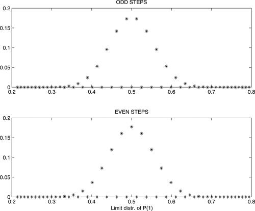
Thus, the figure indicates that both stationary distributions are centered around 0.5 (hence, corresponding limit distributions of a_t have centers around zero). Further, it was revealed that the limit distribution does not depend on initial a₁, however it depends on c: though the mean still tends to 0.5, the limit variance is smaller for c closer to zero.

4.1.2. Case with c > 0

Figure 2 shows the limit behavior of distribution of P_t in the case of positive parameter c. It is seen that now the picture is quite different, the figure indicates that the limit distribution is “unproper,” equal to a Bernoulli distribution with certain $\mathcal{P}$ such that $\mathit{Prob}(P_t\to 1)=\mathcal{P},$ while $\mathit{Prob}(P_t\to 0)=1-\mathcal{P}.$ Notice that it corresponds to a_t tending to $\pm \infty ,$ with the same probabilities. Moreover, it was revealed that $\mathcal{P}$ depends on both a₁ and c. The upper subplot of Figure 2 shows the distribution of P_t in the process starting from $a_1=0.2$ and with c = 0.05, after 1000 steps (the limit behavior of the sequence with odd and even steps is comparable). In fact, as it is possible to work computationally just with finite matrices and domains of values, we set values $a=a_1\pm 300·c$ as absorbing states. Regarding the domain of P_t, absorbing states were then $\mathit{Pmin}\approx 4·{10}^{-7},\mathit{Pmax}\approx 1-3·{10}^{-7}.$ Final distribution had E$P_t=0.814653$ (in fact it is the estimate of probability $\mathcal{P}$), Var$P_t=0.1508043,$ while E$P_t·(1-$ E$P_t)=0.1508045$ (this could be taken as an indication how close we are already to Bernoulli distribution).

Figure 2. Approximate limit distribution of P_t: Above for $a_1=0.2,c=0.05,$ below for $a_1=-0.1,c=0.05.$

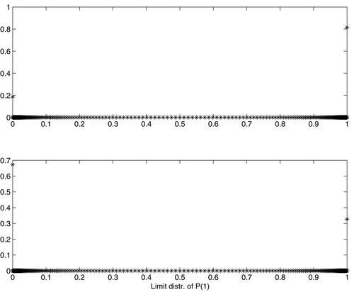
The lower subplot of Figure 2 shows the same for the case with $a_1=-0.1,c=0.05.$ Now, after 1000 steps and with absorbing states constructed as above, we obtained E$P_t=0.327023,$ Var$P_t=0.2200786,$ while E$P_t·(1-$ E$P_t)=0.2200789.$

5. Time dependent parameters

In many instances the impact of walk history to its future steps could be changing during observation period and therefore the time-dependent parameters $c_1=c_1(t),c_2=c_2(t)$ should be considered. Then $d=c_1-c_2=d(t)$ as well. It opens a question of their flexible estimation. The problem is solved quite similarly as in other regression model cases: Either the parameters-functions are approximated by certain functional types (polynomial, combination of basic functions, and regression splines) or constructed by a smoothing method, similar to moving window or kernel regression approach. The method described in Murphy and Sen (1991) is of such a type and concerns the Cox regression model. All these approaches can again be incorporated to the logistic model form, just the number of parameters will be larger. For instance, in the following examples we shall use cubic polynomials for both estimated “parameters” $c_2,d$ (hence $c_1=c_2+d$ will also be a cubic polynomial), each will be given by four parameters of cubic curve.

Further, in the last example the non-parametric moving window ML method was used as well. The estimation procedure started from an initial estimate of parameter a₁ (obtained e.g. from constant model or polynomial model described above). Then both $c_2(t)$ and d(t) were estimated like constant parameters, however with data weighted by a Gauss kernel centered sequentially at M time points $T(m),m=1,2,..,M$ selected inside $[1,T].$ In such a way a preliminary rough estimates of values $c_2(T_{(m)}),d(T(m))$ were obtained. After that, these rough estimates were smoothed secondary, again with a Gauss kernel, to obtain smooth curves of $c_2(t),d(t)$ given at all $t=1,2,\dots T.$ In the end, the final ML estimate of a₁ with $c_2(t),d(t)$ already fixed was computed. The procedure result depends on the choice of “window width” parameter, that is, the standard deviation of Gauss density used as the kernel parameter. By the way, even the Matlab function glmfit.m is able to work with different weights assigned to each data-point.

Another often used method dealing with time-dependent parameters is based on the Bayes approach, it treats each such time-evolving parameter as a random dynamic sequence with a prior model of its development (Gamerman and West 1987).

6. Numerical examples

The objective is, first, to study the behavior of processes, and, second, to examine how well the MLE performs in the case of constant parameters as well as in the case when they are time-evolving.

6.1. Artificial data

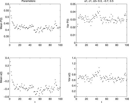
In the first example the data were generated from the model with initial $a_1=0.3$ and constant parameters $c_1=-0.7,c_2=0.5.$ Two cases were compared, in the first one just 20 walks of length 20 steps were generated. The MLE yielded the following estimates (their standard errors based on approximate normality of the MLE are in parentheses): $$a_1=0.3996(0.2133),c_2=0.5869(0.0887),d=-1.4802(0.2017),$$ hence $c_1=c_2+d=-0.8214(0.1116).$

It is seen that even for this case with small number of observations the estimates are quite reasonable, except that the standard error for a₁ is rather large (P-value of the test of nullity of a₁ equals 0.0610).

In the second attempt with the same model, 100 walks, each with 100 steps, were generated. Now the results of the MLE are much more precise: $$a_1=0.3007(0.0454),c_2=0.5057(0.0151),d=-1.2173(0.0362),c_1=c_2+d=-0.7099(0.0211).$$

Figure 3 then shows the development of a_t and P_t, namely their averages and variances from generated 100 walks. It is seen that both stabilize rather quickly, as a consequence of negative c₁ and positive c₂ reducing $P_{t+1}$ after event X_t = 1 and increasing it after X_t = 0.

Figure 3. Sample means and variances of a_t and P_t.

6.2. Parameters as functions of time

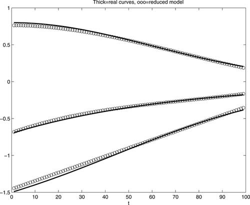
In the next simulated example functional “parameters” were considered. Namely, walks had again length 100 steps, $a_1=-0.2,$ the first $c_1(t)=-0.7·{(0.25)}^{(t/100)}$ was increasing exponential curve, the second $c_2(t)=0.8·{(0.25)}^{{(t/100)}^2}$ was decreasing S-curve. Again, 100 such walks were generated. Functions $c_1(t)$ and $d(t)=c_1(t)-c_2(t)$ were estimated as cubic polynomials, in the logistic model framework. Results, a sufficiently good approximation to real curves, are seen from Figure 4. Initial a₁ was estimated as −0.1464, with P-value of its nullity test 0.1468 (hence, its nullity cannot be rejected). These results, however, correspond to the full model, some parameters of both cubic curves were not significant, therefore a sequential reduction of the model was performed. Namely, at each reduction step one of the components with non-significant parameters (i.e. the one with the largest p-value of the test based on the MLE asymptotic normality) was removed from the model. Thus, the final model, with all components significant, had functions $c_2(t)={\alpha }_0+{\alpha }_2{t}^2+{\alpha }_3{t}^3$ and $d(t)={\beta }_0+{\beta }_{1}t.$ The values of estimates were $a_1=-0.1553$ (p-value = 0.0283), further ${\alpha }_0=0,7640,{\alpha }_2=-0,00011,{\alpha }_3=4,8e-07,{\beta }_0=-1,4560,{\beta }_1=0,0111,$ all corresponding p-values were already quite negligible. Figure 5 shows the results of this last model.

Figure 4. Functional parameters (thick lines, from above $c_2(t),c_1(t),d(t)=c_1(t)-c_2(t)$) and their estimates with complete cubic functions (circles).

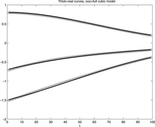
Figure 5. Functional parameters (thick) and their estimates via reduced cubic model (circles).

6.3. Real data case

The following data are taken from Exercise 16.1 of Meeker and Escobar (1998). The data are records of problems (failures, troubles) with 10 computers, each followed for 105 days. The table displays the computer number and then days of reported and repaired troubles.

401: 18, 22, 45, 52, 74, 76, 91, 98, 100, 103.

402: 11, 17, 19, 26, 27, 38, 47, 48, 53, 86, 88.

403: 2, 9, 18, 43, 69, 79, 87, 87, 95, 103, 105.

404: 3, 23, 47, 61, 80, 90.

501: 19, 43, 51, 62, 72, 73, 91, 93, 104, 104, 105.

502: 7, 36, 40, 51, 64, 70, 73, 88, 93, 99, 100, 102.

503: 28, 40, 82, 85, 89, 89, 95, 97, 104.

504: 4, 20, 31, 45, 55, 68, 69, 99, 101, 104.

601: 7, 34, 34, 79, 82, 85, 101.

602: 9, 47, 78, 84.

Thus, from our point of view, 10 walks, each of length 105 time units, were observed. Steps X_t = 1, representing the events = reported troubles, were rather sparse, just 91, in the rest of days X_t = 0, that is, nothing has occurred. Nevertheless, it could be expected that the wear of devices was increasing.

First, the model with constant parameters was fitted. The results were the following (again with asymptotic standard deviations in parentheses): $$a_1=-3.0368(0.2578),c_2=0.0122(0.0062),d=-0.0145(0.0640),$$ hence $c_1=c_2+d=-0.0022(0.0592).$

It is seen that $c_1<0,$ though non-significantly, which means that after a failure and repair the probability of further failure decreased slightly. On the other hand, positive c₂ means that the probability of failure increases in time, linearly in the framework of model with constant parameters. Achieved maximal log-likelihood value equaled −295.54.

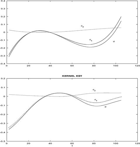
In the next attempt, the model allowing cubic dependence of both $c_1(t),c_2(t)$ on time was applied. Its maximum likelihood estimate was obtained, however the most of the parameters were not statistically significant, that is, they were close to zero and corresponding normal tests of their nullity had large p-values. Again, the model was then reduced sequentially, at each step the parameter with the largest (and larger than 0.1) p-value was eliminated. Quite astonishingly, this procedure lead to a rather plain model with $c_2(t)=\beta ·t^2$ and function d(t) omitted, namely $a_1=-2.7797,\beta =3.2931e-06,$ corresponding p-values were $3e-63,0.0003.$ It means that in fact $c_1(t)=c_2(t),$ an interpretation is that the influence of events X_t = 1 is rather negligible and the probability of such events is increasing (slightly, but significantly) in time. In fact, its logit a(t) increases cubically, as from expression (2) we have now that $a_{t+1}=a_1+\beta {\sum }_{s=1}^t{s}^2.$ On the other side, while the maximum likelihood corresponding to the full cubic model was −292.49, the value achieved by the reduced model was slightly smaller, −293.86.

Finally, the moving window method was utilized, too. Figure 6 shows both the full cubic model in its upper subplot and the mowing window estimates, in lower subplot. It is seen that they are quite comparable. Final estimate of parameter $a_1=-2.7189,$ the maximum of log-likelihood was −293.42. It is seen that the results of all these models, including the model with constant parameters, were quite comparable in terms of maximal log-likelihood. On the other side, certain differences of their fit can be traced from the following graphical analysis.

Figure 6. Estimates of model functions. Above: full cubic model, below: moving window estimates.

6.4. Graphical test of model fit

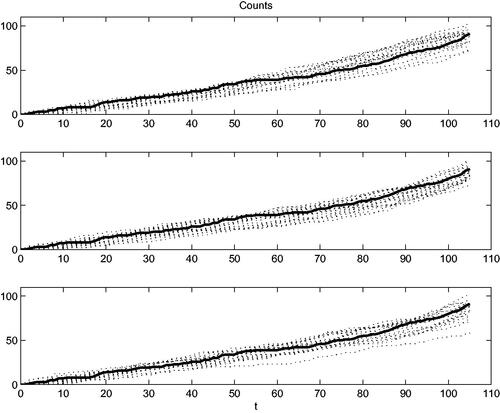
In general, the objective of goodness-of-fit tests is to decide whether the model corresponds to observed data. There are several possibilities, consisting mostly of the comparison of certain characteristics of observed data with the same characteristics derived from the model. We decided to consider, as the characteristics suitable for graphical comparison, the cumulated processes of steps of all walks together. In our case it equals $\mathcal{N}(t)={\sum }_{i=1}^N\sum _{s\le t}{X}_i(s),$ which is in fact the process counting observed events, the discrete-time counting process.

A good model should be able to generate comparable sequences of events. Therefore, when new walks (the same number and length) are generated from the model, their aggregated counting process should be similar to process observed. When such a generation is done many times, a “cloud” of counting processes is obtained. In the graphical test form, this cloud of processes generated from the model should be around the process obtained from data. It is illustrated on the next Figure 7. All three models presented above were compared with real data. It is seen that the constant model (upper plot) underestimates (from the beginning) and overestimates (for larger times) the real process development. The other two models perform better, the full cubic model’s fit (middle plot) does not seem to be worse than the non-parametric model in the lower plot.

Figure 7. Thick curve = real observed counting process of failures. Clouds of dotted curves = counting processes generated from estimated models. Top: constant model, middle plot: full cubic model, bottom: model from mowing window estimates.

7. Concluding remarks

Standard non-parametric estimator in the count data setting is the Nelson-Aalen estimator of the cumulative hazard function. In the case of our real data example it is given by observed counting process $\mathcal{N}(t)$ divided by the number of objects, as all objects are “at risk” during the whole observation period. However, such an estimator does not take into account possible dependence of future risk on objects history. It could be incorporated via a regression model modeling the hazard rate change after occurred event. Hence, hazard function is in fact a random function.

Models proposed in the present article offer an explicit description of such an impact of process history to actual count probabilities. A generalization may consist of considering a longer memory, we have explored just models with memory 1. Further generalization could include an influence of covariates to probability logits. The model’s form makes it easy to model using logistic regression. On the other hand, from this point of view certain observable events from the process history could be taken as covariates, too. In models studied here, this role is played by the last preceding process value.

Statistical analysis of processes of recurrent events has, moreover, to take into account possible heterogeneity of studied objects, in particular when dealing with medical, demographic or also with economic data (see e.g. Winkelmann 2008, Ch. 4). In such a case, an additional random effect variable (called also the frailty variable) should be added to the logit model. Procedure of estimation then uses an alternation of two steps estimating frailty values and the rest of model, respectively. Thus, the concept of heterogeneity offers another way how the models studied in the present article could be enriched.

Additional information

Funding

The research was supported by the grant No. 18-02739S of the Grant Agency of the Czech Republic.

References

- Davis, R. A., and H. Liu. 2016. Theory and inference for a class of observation-driven models with application to time series of counts. Statistica Sinica 26:1673–707. doi:10.5705/ss.2014.145t.
- Gamerman, D., and M. West. 1987. An application of dynamic survival models in unemployment studies. The Statistician 36 (2/3):269–74. doi:10.2307/2348523.
- Hawkes, A. G. 1971. Spectra of some self-exciting and mutually exciting point processes. Biometrika 58 (1):83–90. doi:10.1093/biomet/58.1.83.
- Kouřim, T. 2019. Random walks with memory applied to grand slam tennis matches modeling. In Proceedings of MathSport International 2019 Conference (e-Book). Propobos Publications, 220–7.
- Kouřim, T., and P. Volf. 2020. Discrete random processes with memory: Models and applications. Applications of Mathematics 65 (3):271–86. doi:10.21136/AM.2020.0335-19.
- Meeker, W. Q., and L. A. Escobar. 1998. Statistical methods for reliability data. New York: Wiley.
- Moeller, T. A. 2016. Self-exciting threshold models for time series of counts with a finite range. Stochastic Modeling 32:77–98.
- Murphy, S. A., and P. K. Sen. 1991. Time-dependent coefficients in a Cox-type regression model. Stochastic Processes and Their Applications 39 (1):153–80. doi:10.1016/0304-4149(91)90039-F.
- Weiss, C. H. 2018. An introduction to discrete valued time series. New York: Wiley.
- Winkelmann, R. 2008. Econometric analysis of count data. Berlin: Springer.