A robust Spearman correlation coefficient permutation test

Abstract

In this work, we show that Spearman’s correlation coefficient test about $H_0:{\rho }_s=0$ found in most statistical software is theoretically incorrect and performs poorly when bivariate normality assumptions are not met or the sample size is small. There is common misconception that the tests about ${\rho }_s=0$ are robust to deviations from bivariate normality. However, we found under certain scenarios violation of the bivariate normality assumption has severe effects on type I error control for the common tests. To address this issue, we developed a robust permutation test for testing the hypothesis $H_0:{\rho }_s=0$ based on an appropriately studentized statistic. We will show that the test is asymptotically valid in general settings. This was demonstrated by a comprehensive set of simulation studies, where the proposed test exhibits robust type I error control, even when the sample size is small. We also demonstrated the application of this test in two real world examples.

Keywords:

• Rank correlation
• studentized
• small sample
• non-normality

1. Introduction

The concept of correlation and regression was originally conceived by Galton when studying how strongly the characteristics of one generation of living things manifested in the following generation (Stanton 2001). The ideas prompting the development of more mathematically rigorous treatment of correlation were developed by Karl Pearson in 1896, which yielded the well-known Pearson Product Moment Correlation Coefficient (Pearson 1896) given as (1) $$\rho (X,Y)=\frac{\mathit{\text{Cov}}(X,Y)}{{\sigma }_X{\sigma }_Y}=\frac{E(X-{\mu }_X)(Y-{\mu }_Y)}{\sqrt{E{(X-{\mu }_X)}^{2}E{(Y-{\mu }_Y)}^2}},$$(1) where X and Y are two random variables from a non-degenerative joint distribution F_XY, Cov(X, Y) denotes the covariance, and μ_X and μ_Y, σ_X and σ_Y are the population means and standard deviations, respectively. If we let (X₁, Y ₁), $(X_2,Y_2),\cdots ,(X_n,Y_n)$ denote n paired i.i.d. observations, then the sample Pearson correlation coefficient is given as (2) $$r(X,Y)=\frac{{\Sigma }_{i=1}^n(X_i-\overline{X})(Y_i-\overline{Y})}{\sqrt{{\Sigma }_{i=1}^n{(X_i-\overline{X})}^2}\sqrt{{\Sigma }_{i=1}^n{(Y_i-\overline{Y})}^2}},$$(2) where $\overline{X}$ and $\overline{Y}$ are the sample means of X and Y, respectively.

Shortly after Pearson’s work was published, Spearman introduced the rank correlation coefficient in 1904. The Spearman correlation has advantages of being robust to extreme values and disparities between the marginal distributions between two variables (Spearman 1961). However, it should be noted that K. Pearson, in his biography of Galton, says that the latter “dealt with the correlation of ranks before he even reached the correlation of variates, i.e., about 1875”, but Galton apparently did not publish anything explicitly about this result (Kendall and Stuart 1979). Mathematically, Spearman’s correlation coefficient is defined as the Pearson correlation coefficient on the ranks of (X₁, Y₁), $(X_2,Y_2),\cdots ,(X_n,Y_n)$ and denoted as (3) $${\rho }_s(X,Y)=\rho (a,b),$$(3) where $a_i=\mathit{\text{Rank}}(X_i)$ and $b_i=\mathit{\text{Rank}}(Y_i)$ are the ranks of X_i and Y_i, respectively, $i=1,2,\cdots ,n.$ In general, when discussing the Spearman correlation coefficient little attention is given to its population measure. However, if we consider that $a_i/n$ converges to $F(X_i),$ then one may consider the population measure linked to Spearman’s sample correlation coefficient as, (4) $$\begin{array}{c}{\rho }_s(X,Y)=\frac{E\{F_X(X)-E[F_X(X)\left]\right\}\{F_Y(Y)-E[F_Y(Y)\left]\right\}}{\sqrt{E{\{F_X(X)-E[F_X(X)\left]\right\}}^2}\sqrt{E{\{F_Y(Y)-E[F_Y(Y)\left]\right\}}^2}}\\ =\frac{E[F_X(X)-\frac{1}{2}][F_Y(Y)-\frac{1}{2}]}{\sqrt{E{[F_X(X)-\frac{1}{2}]}^2}\sqrt{E{[F_Y(Y)-\frac{1}{2}]}^2}},\end{array}$$(4) where F_X and F_Y are the marginal cumulative distribution functions (CDFs) for X and Y, respectively. The expectation E is taken over the joint distribution F(X, Y). The sample estimator of ρ_s can be obtained by replacing the original observations with their ranks in Equation (2)(2) $$r(X,Y)=\frac{{\Sigma }_{i=1}^n(X_i-\overline{X})(Y_i-\overline{Y})}{\sqrt{{\Sigma }_{i=1}^n{(X_i-\overline{X})}^2}\sqrt{{\Sigma }_{i=1}^n{(Y_i-\overline{Y})}^2}},$$(2) , (5) $$\begin{array}{c}{r}_s(X,Y)=r(a,b)=\frac{{\Sigma }_{i=1}^n(a_i-\overline{a})(b_i-\overline{b})}{\sqrt{{\Sigma }_{i=1}^n{(a_i-\overline{a})}^2}\sqrt{{\Sigma }_{i=1}^n{(b_i-\overline{b})}^2}}\\ =1-\frac{6{\Sigma }_{i=1}^n{(a_i-b_i)}^2}{n(n^2-1)}.\end{array}$$(5)

For samples from a bivariate normal population, there is also a known relation between the Spearman and Pearson correlation coefficients (Moran 1948), which is (6) $$E(r_s)=\frac{6}{\pi (n+1)}\{{\hspace{0.17em}\text{sin}\hspace{0.17em}}^{-1}\rho +(n-2){\hspace{0.17em}\text{sin}\hspace{0.17em}}^{-1}\frac{1}{2}\rho \}.$$(6)

While Pearson’s ρ measures the linear relationship between two random variables it is often described that Spearman’s ρ_s measures the strength and direction of association between X and Y monotonically, thus it may be considered a more general measure of association, albeit it does measure the linear association between F(X) and F(Y). Spearman’s correlation coefficient is also less sensitive to extreme values because it is rank based. Due to these advantages, it is widely used as a measure of association between two measurements. It is often of interest to test whether two random variables are correlated, i.e., $H_0:{\rho }_s=0.$ The common methods include (1)(1) $$\rho (X,Y)=\frac{\mathit{\text{Cov}}(X,Y)}{{\sigma }_X{\sigma }_Y}=\frac{E(X-{\mu }_X)(Y-{\mu }_Y)}{\sqrt{E{(X-{\mu }_X)}^{2}E{(Y-{\mu }_Y)}^2}},$$(1) a t-distribution based test, (2)(2) $$r(X,Y)=\frac{{\Sigma }_{i=1}^n(X_i-\overline{X})(Y_i-\overline{Y})}{\sqrt{{\Sigma }_{i=1}^n{(X_i-\overline{X})}^2}\sqrt{{\Sigma }_{i=1}^n{(Y_i-\overline{Y})}^2}},$$(2) a test based on Fisher’s Z transformation, and (3)(3) $${\rho }_s(X,Y)=\rho (a,b),$$(3) what we term the naive permutation test.

The t-distribution based test is commonly used when the sample size is large, with the t-statistic defined as $$t=r_s\sqrt{\frac{n-2}{1-r_s^2}}.$$

This statistic was first used for Pearson’s correlation coefficient. Under bivariate normality assumptions it approximately follows student’s t distribution with n − 2 degrees of freedom under H₀ (Edgell and Noon 1984). When used for Spearman’s ρ_s, this test incorrectly based on the approximate bivariate normality of the ranks. For the test based on Fisher’s Z transformation, the statistic is defined as $$Z=\frac{1}{2}\text{arctanh}(r_s)=\frac{1}{2}\text{ln}\hspace{0.17em}\frac{1+r_s}{1-r_s}.$$

Under bivariate normality assumptions the transformed Z statistic approximately follows normal distribution $N(0,\frac{1.06}{n-3})$ under H₀ (Fieller, Hartley, and Pearson 1957).

Permutation tests have been applied in a broad range of scenarios (Pauly and Smaga 2020). For small sample size cases, naive permutation tests are also often used for testing ρ_s, where $\{X_i,i=1,\dots ,n\}$ and $\{Y_i,i=1,\dots ,n\}$ are randomly shuffled separately and independently to simulate the sample distribution of r_s under H₀, which may be an invalid test for testing $H_0:{\rho }_s=0$ given $G(F(X),F(Y))=G(F(X))G(F(Y))$ does not imply ${\rho }_s=0,$ where $G(·,·)$ denotes the joint CDF of $F(X),F(Y).$ For example, Marozzi proposed a permutation test for Kendall W coefficient, which is a rank-based measure of concordance between multiple criteria (Marozzi 2014). When there are only two judges, the Kendall W is a linear transformation of ρ_s, so the tests on these two coefficients are equivalent. However, similar to the naive permutation test, the method did not account for the difference between independence and zero correlations.

These tests are so widely used that they are often the default options in common statistical software packages such as R (R Core Team 2013) and SAS (SAS Institute 2015). Both software packages (cor.test function for R and CORR procedure for SAS) by default uses the t-distribution based test, as shown in their documentations. However, there is little discussion that these tests rely on the untenable assumption that the underlying sample distribution of the ranks has a bivariate normal distribution, which is in fact an impossibility. Even among those who noted this assumption, there is a misconception that the above tests are robust to such deviations because Spearman’s ρ_s is rank based. This is exemplified in a discussion by Fieller et al. in their article (Fieller, Hartley, and Pearson 1957),

“Conversely, starting from any bivariate distribution $\varphi (X,Y)$ we can always find monotonic transformations $X=f(x),\hspace{0.17em}Y=g(y)$ to standardized normal variates x and y. The resulting bivariate distribution $\psi (X,Y)$ will not necessarily be bivariate normal, but we think it likely that in practical stations it would not differ greatly from this form. This is a field in which further investigation would be of considerable interest.”

However, as we will show in Section 3, all the commonly used tests about ${\rho }_s=0$ as discussed above, including the naive permutation test, are not even asymptotically valid when the exchangeabilty assumptions are violated under H₀. That is, even when $n\to \infty ,$ the type I error cannot be controlled at the desired level. In some cases, the type I error can severely drift away from the desired level as the sample size increases! An undesirable feature that is more notable in the era of “big-data”. Another variation of this approach is the Fisher-Yates coefficient, which transforms the original X and Y to their corresponding normal quantiles before the testing (Fisher and Yates 1938). Although the marginal distributions of the transformed variates take a pseudo normal form, the joint normality of these transformed values is not guaranteed.

In terms of our modified permutation test it is important to note the classic large sample result in Serfling where the “distribution free” large sample normal approximation for the sampling distribution for Pearson’s sample correlation coefficient r is derived using the multivariate delta method (Kendall and Stuart 1979). This method guarantees type I error converges to α when $n\to \infty$ given finite fourth moments. A straightforward way to obtain a similar result for Spearman’s correlation is given by replacing the (X_i, Y_i) with (a_i, b_i). The test is asymptotically valid because the ranks are asymptotically independent, as we will discuss in Section 2. Even though large sample approximations about these estimators are asymptotically valid they tend to suffer inflated type I errors in the small sample setting, e.g., n < 50.

Permutation tests provide a strong alternative testing approach. The permutation approach has been applied to a variety of univariate and multivariate problems and its properties have been extensively studied (Giancristofaro and Bonnini 2008; Arboretti Giancristofaro, Bonnini, and Pesarin 2009; Pesarin and Salmaso 2010a; Basso and Salmaso 2011; Pesarin and Salmaso 2012, 2013; Arboretti et al. 2014; Giancristofaro 2014; Salmaso, 2015). For an overview of permutation tests, please see Salmaso and Pesarin (2010) and Pesarin and Salmaso (2010b). Recently, DiCiccio and Romano have shown that the permutation distribution of Pearson’s correlation coefficient does not converge to the sampling distribution when two random variables are dependent but uncorrelated (DiCiccio and Romano 2017). Therefore, a a simple permutation test ignoring possible dependency structures can lead to invalid inference about the Pearson’s and related correlation coefficients (DiCiccio and Romano 2017; Hutson and Yu 2021).

In this work, we show that a naive permutation test of ρ_s suffers a similar problem. To address this issue, we propose a studentized permutation test for Spearman’s correlation ρ_s, which extends the work or Diccicio and Romano for Pearson’s correlation coefficient ρ (DiCiccio and Romano 2017). We will show that the proposed test is asymptotically valid under general assumptions and is exact under exchangeability assumptions when $G(F(X),F(Y))=G(F(X))G(F(Y)),$ i.e., more simply when X and Y are independent. We show that our newly proposed test has robust Type I error control even when the exchangeability assumption does not hold and the sample distribution is non-normal. Importantly, even when the sample size is as small as 10, the type I error is still well controlled, which is advantageous over the tests based on large sample approximations. This will be illustrated by a set of simulation studies. Finally, we will demonstrate the application of this test in real world examples of transcriptomic data of TCGA breast cancer patients, as well as a data set of PSA levels and age.

2. Methods

2.1. Spearman’s permutation correlation test

Spearman’s coefficient ${\rho }_s(X,Y)$ is the Pearson correlation coefficient of the ranks of X and Y, that is $\rho (a,b).$ When there are ties in the data, the tied ranks are typically taken as an average. Unlike Pearson’s correlation coefficient ρ, which measures the linear relationship between two random variables, Spearman’s correlation coefficient ρ_s measures a monotonic association, thus is far less restrictive. Note that Spearman’s correlation coefficient is also the linear measure between F(X) and F(Y). It is also less sensitive to non-normality or extreme values.

Despite the above advantages, it is a misconception that the tests of ${\rho }_s=0$ based on the bivariate normality assumptions underlying the original data will be robust to the deviation from this assumption. In fact, tests of ρ_s typically suffer similar issue as for ρ. We also emphasize that “normality” refers to the joint normality as opposed to marginal normality, because two random variables that are marginally normal can have a joint non-normal distribution. Therefore, the Fisher-Yates coefficient, which back transforms a variables rank through the normal quantile function does not provide what heuristically one may consider as a simple correction. In Section 3, we will empirically show that violation of the joint normality assumption will have severe effect on type I error control. In addition, it is in fact impossible for the joint distribution of the ranks to be bivariate normal.

Our approach is to replace the observations (X_i, Y_i) with their ranks (a_i, b_i) in order to develop a Spearman’s correlation permutation test analog to the Pearson’s correlation permutation test, with some subtle differences. The studentized permutation test of the Pearson’s ρ proposed by DiCiccio and Romano only requires finite fourth moments and that the paired observations are i.i.d (DiCiccio and Romano 2017), i.e., (X_i, Y_i) and (X_j, Y_j) are independent and identically distributed when $i\ne j.$ However, it should be noted the ranks (a_i, b_i) and (a_j, b_j) are no longer independent pairs. For example, suppose we have n = 2, then after knowing $(a_1,b_1)=(1,1)$ we will immediately know $(a_2,b_2)=(2,2).$

In spite of this, we can show that (a_i, b_i) and (a_j, b_j) are asymptotically independent and follow identical distributions when $i\ne j.$ This result follows naturally from the convergence of empirical CDF to CDF. Without loss of generality, we start by considering a single variable X. Since X_i and X_j are i.i.d. observations, we have $W_i=F(X_i),\hspace{0.17em}{W}_j=F(X_j)$ being i.i.d as well, so $F(W_i,W_j)=F(W_i)F(W_j).$ Also we have a_i and a_j being the ranks of X_i and X_j, so $a_i=n\widehat{F}(X_i)$ and $a_j=n\widehat{F}(X_j),$ where $\widehat{F}$ is the empirical CDF of X. By the Strong Law of Large Numbers, we have $(\widehat{F}(X_i),\widehat{F}(X_i))\to (W_i,W_j)$ almost surely, thus $a_i/n,$ and $a_j/n$ converge almost surely to a pair of independent variables W_i and W_j. Therefore, a_i and a_j are asymptotically independent. Note that this result is on two observations of the same random variable, i.e., a_i and a_j. It does not concern the dependency between X_i and Y_i, or between a_i and b_j.

It is obvious that a_i and a_j follow the same distribution, and the same conclusion applies to b_i and b_j. Therefore, two paired observations (a_i, b_i) and (a_j, b_j) are identically, and asymptotically independently distributed when $i\ne j.$ Consequently, the exchangeability condition of i.i.d observations holds asymptotically, so the test will be asymptotically exact.

With the above results, the one-sided studentized permutation test for testing $H_0:{\rho }_s=0$ versus $H_1:{\rho }_s>0$ is performed by the following steps. The test is implemented in the R perk (permutation tests of correlation c(k)oefficients) package, which will be available on CRAN (The Comprehensive R Archive Network, https://cran.r-project.org/) and GitHub (https://github.com/hyu-ub/perk).

1. For n paired i.i.d. observations (X₁, Y₁), $(X_2,Y_2),\cdots ,(X_n,Y_n),$ calculate their ranks within each random variable, (a₁, b₁), $(a_2,b_2),\cdots ,(a_n,b_n).$

2. Estimate the Spearman’s ρ_s using Equation (5)(5) $$\begin{array}{c}{r}_s(X,Y)=r(a,b)=\frac{{\Sigma }_{i=1}^n(a_i-\overline{a})(b_i-\overline{b})}{\sqrt{{\Sigma }_{i=1}^n{(a_i-\overline{a})}^2}\sqrt{{\Sigma }_{i=1}^n{(b_i-\overline{b})}^2}}\\ =1-\frac{6{\Sigma }_{i=1}^n{(a_i-b_i)}^2}{n(n^2-1)}.\end{array}$$(5) as r_s.

3. Estimate the variance of sample estimates r_s by $$\begin{array}{c}{\widehat{\tau }}_n^2=\frac{{\widehat{\mu }}_{22}}{{\widehat{\mu }}_{20}{\widehat{\mu }}_{02}},\\ {\widehat{\mu }}_{\mathit{\text{pq}}}=\frac{1}{n}\sum _{i=1}^n{(a_i-\overline{a})}^p{(b_i-\overline{b})}^q.\end{array}$$

4. Calculate the studentized statistic $R_s=r_s/{\widehat{\tau }}_n.$

5. Randomly shuffle $\{b_1,b_2,\dots ,b_n\}$ for B times. For each permutation, calculate the permuted studentized statistic $R_s^k,\hspace{0.17em}k\in \{1,\dots ,B\}.$ Note that ${\widehat{\tau }}_n^2$ needs to be calculated for each permutation because ${\widehat{\mu }}_{22}$ is not permutation invariant. Specifically, for permutation π, we have $$\begin{array}{c}{\widehat{\mu }}_{22}^{*}=\frac{1}{n}\sum _{i=1}^n{(a_i-\overline{a})}^2{(b_{\pi (i)}-\overline{b})}^2,\\ {\widehat{\tau }}_n^{2(*)}=\frac{{\widehat{\mu }}_{22}^{*}}{{\widehat{\mu }}_{20}{\widehat{\mu }}_{02}}.\end{array}$$

6. Calculate the p-value by $$p=\frac{1}{B}{\Sigma }_{k=1}^{B}I(R_s^k>R_s).$$

7. Reject H₀ if $p\le \alpha .$

3. Simulations

We examined the Type I error control across all of the tests introduced above using distributions commonly found in the literature for these examinations across a wide range of settings (Figure 1) (DiCiccio and Romano 2017; Hutson 2019). For our simulation study, we focused on testing $H_0:{\rho }_s=0$ versus $H_1:{\rho }_s>0,$ with sample sizes $n=10,25,50,100,200.$ Each simulation utilized 10, 000 Monte Carlo replications and the number of permutations used is 1, 000. We compared the t test, Fisher’s Z-transformation (Fisher’s Z), Fisher-Yates method, Serfling’s large sample normal approximation (Asymp Norm), naive permutation test (Permute), and studentized permutation test (Stu Permute). The Type I error control for $\alpha =0.05$ was examined. The simulation scenarios 1 through 5 from DiCiccio and Romano. Two additional distributions were studied as well:

1. Multivariate normal (MVN) with mean zero and identity covariance.

2. Exponential given as $(X,Y)=r{S}^{T}u$ where $S=\mathit{\text{diag}}(\sqrt{2},1),\hspace{0.17em}r\sim \hspace{0.17em}\text{exp}(1),$ and u is uniformly distributed on the two dimensional unit circle.

3. $t_{4.1}$ where $X=W+Z$ and $Y=W-Z,$ where W and Z are iid $t_{4.1}$ random variables.

4. Circular given as the uniform distribution on a two dimensional unit circle.

5. Multivariate t-distribution (MVT) with 5 degrees of freedom.

6. Mixture of two bivariate normal distributions given as $(X,Y)=W{Z}_1+(1-W)Z_2$ where $W\sim \mathit{\text{Bernoulli}}(0.5),\hspace{0.17em}{Z}_1\sim N((\begin{array}{c}0\\ 0\end{array}),(\begin{array}{cc}1& \rho \\ \rho & 1\end{array})),\hspace{0.17em}{Z}_2\sim N((\begin{array}{c}0\\ 0\end{array}),(\begin{array}{cc}1& -\rho \\ -\rho & 1\end{array})).$ We select a range of ρ’s: 0.1, 0.3, 0.6 and 0.9 to simulate different degrees of dependencies between X and Y (MVN 1, MVN 3, MVN6, MVN 9).

7. Mixture of four bivariate normal distributions (MVN 45), given as $(X,Y)={\Sigma }_{k=1}^{4}I(W=k)Z_k$ where $P(W=k)=0.25,\hspace{0.17em}k=1,2,3,4.$ In addition, $Z_k\sim N({\mu }_k,I_2),$ where ${\mu }_1={(5,5)}^T,\hspace{0.17em}{\mu }_2={(5,-5)}^T,\hspace{0.17em}{\mu }_3={(-5,5)}^T,\hspace{0.17em}{\mu }_4={(-5,-5)}^T.$

The results in Table 1 and Figure 2 show that the large sample asymptotic normal approximation has inflated type I error rates for all distributions when $n\le 50.$ The t test, Fisher’s Z test, Fisher-Yates, and naive permutation tests tend to be over-conservative for the exponential and circular distributions. While for the $t_{4.1}$ distribution, the type I error is consistently inflated. Note that, for these tests, such deviation cannot be corrected as sample size increases. Instead, they may converge to an arbitrary level, either lower or higher than α.

Table 1. Type I error rate of testing $H_0:{\rho }_s=0$ versus $H_0:{\rho }_s>0.$

Distribution	n	t test	Fisher’s Z	Fisher-Yates	Asymp Norm	Permute	Stu Permute
MVN	10	0.0498	0.0420	0.0479	0.1223	0.0495	0.0457
	25	0.0501	0.0444	0.0499	0.0811	0.0494	0.0487
	50	0.0512	0.0473	0.0509	0.0639	0.0508	0.0525
	100	0.0529	0.0484	0.0527	0.0596	0.0530	0.0518
	200	0.0479	0.0438	0.0493	0.0525	0.0487	0.0496
Exponential	10	0.0707	0.0623	0.0813	0.1300	0.0715	0.0479
	25	0.0744	0.0689	0.0914	0.0804	0.0741	0.0492
	50	0.0795	0.0724	0.1061	0.0680	0.0798	0.0509
	100	0.0772	0.0706	0.0975	0.0561	0.0774	0.0497
	200	0.0789	0.0735	0.0998	0.0549	0.0785	0.0509
$t_{4.1}$	10	0.0625	0.0531	0.0693	0.1275	0.0606	0.0489
	25	0.0631	0.0574	0.0846	0.0768	0.0629	0.0480
	50	0.0631	0.0579	0.0910	0.0614	0.0628	0.0457
	100	0.0677	0.0611	0.1082	0.0567	0.0672	0.0491
	200	0.0728	0.0675	0.1149	0.0572	0.0731	0.0521
Circular	10	0.0124	0.0095	0.0041	0.0907	0.0124	0.0514
	25	0.0052	0.0040	0.0004	0.0620	0.0048	0.0474
	50	0.0031	0.0024	0.0001	0.0575	0.0030	0.0487
	100	0.0021	0.0015	<0.0001	0.0537	0.0024	0.0497
	200	0.0016	0.0009	<0.0001	0.0489	0.0020	0.0482
MVT	10	0.0582	0.0502	0.0626	0.1305	0.0584	0.0497
	25	0.0596	0.0543	0.0726	0.0825	0.0602	0.0496
	50	0.0542	0.0489	0.0700	0.0608	0.0553	0.0456
	100	0.0584	0.0535	0.0740	0.0566	0.0574	0.0496
	200	0.0590	0.0539	0.0852	0.0527	0.0590	0.0496
MVN 1	10	0.0541	0.0458	0.0499	0.1271	0.0531	0.0534
	25	0.0484	0.0451	0.0490	0.0777	0.0482	0.0498
	50	0.0481	0.0428	0.0478	0.0631	0.0484	0.0492
	100	0.0497	0.0452	0.0520	0.0564	0.0498	0.0497
	200	0.0495	0.0462	0.0523	0.0529	0.0493	0.0488
MVN 3	10	0.0547	0.0467	0.0539	0.1341	0.0544	0.0497
	25	0.0557	0.0514	0.0607	0.0814	0.0551	0.0516
	50	0.0571	0.0498	0.0607	0.0686	0.0562	0.0508
	100	0.0530	0.0473	0.0651	0.0561	0.0544	0.0497
	200	0.0529	0.0468	0.0603	0.0517	0.0508	0.0473
MVN 6	10	0.0648	0.0555	0.0740	0.1328	0.0643	0.0461
	25	0.0694	0.0624	0.0880	0.0832	0.0686	0.0526
	50	0.0658	0.0606	0.0917	0.0638	0.0650	0.0494
	100	0.0706	0.0644	0.0988	0.0590	0.0694	0.0498
	200	0.0678	0.0615	0.1034	0.0527	0.0667	0.0496
MVN 9	10	0.0944	0.0843	0.1173	0.1405	0.0924	0.0573
	25	0.0932	0.0865	0.1276	0.0829	0.0913	0.0502
	50	0.0965	0.0891	0.1414	0.0662	0.0948	0.0519
	100	0.0997	0.0928	0.1425	0.0593	0.0994	0.0498
	200	0.0950	0.0882	0.1531	0.0536	0.0953	0.0494
MVN 45	10	0.0564	0.0467	0.0487	0.1301	0.0547	0.0515
	25	0.0492	0.0444	0.0480	0.0791	0.0491	0.0482
	50	0.0481	0.0445	0.0507	0.0634	0.0482	0.0512
	100	0.0492	0.0447	0.0498	0.0557	0.0497	0.0488
	200	0.0521	0.0468	0.0492	0.0552	0.0509	0.0519

For MVN 1-9, we simulated a range of dependency among uncorrelated X and Y, where MVN 1 has the weakest and MVN 9 has the strongest dependency (Figure 1). The above four tests showed the type I error rate inflation becomes increasingly severe as the dependency increases. This demonstrates the failure in controlling type I error results from the data being dependent, which can occur when the underlying distribution is non-normal.

Figure 1. Contour plots for the density of a synthetic data set (n = 10, 000) for each simulation distribution.

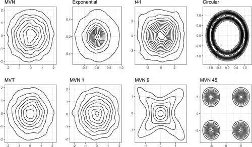
Figure 2. Type I error rate of testing $H_0:{\rho }_s=0$ versus $H_1:{\rho }_s>0.$

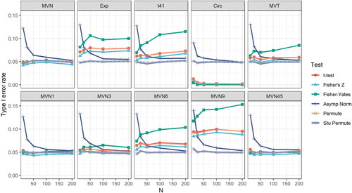
The MVN 45 is a case where the dependency of original data is remedied by using the ranks. In this case, the ranks will distribute as if it comes from a bivariate normal distribution, regardless of the distance between the centers of individual Gaussian sub-populations. Therefore, all four tests show well control of the type I error rate.

On the other hand, the studentized permutation test robustly control type I error for all distributions examined, even when the n is as small as 10. This demonstrates a clear advantage of the proposed test over all other commonly used tests for Spearman’s correlation coefficient.

We also examined the power of different testing methods when ${\rho }_s=0.3$ or 0.6 under the scenario of multivariate normal distributions. For other distributions, most of the tests fail to control the type I error except for the proposed test, so the comparison of power is not meaningful. Table 2 shows that the power of the proposed test is generally lower than that of the t test and naive permutation test, but the difference is generally less than 3%. The exception is when n = 10 and ${\rho }_s=0.6,$ where the loss of power is around 7%. However, this difference quickly diminishes when n increases to 25. On the other hand, the proposed test has a comparable power to Fisher’s Z test in almost all scenarios. These results demonstrate that the proposed test achieve a very robust type I error control at the cost of a small decrease in power.

Table 2. Power of testing $H_0:{\rho }_s=0$ versus $H_0:{\rho }_s>0$ under bivariate normal distributions.

	n	t test	Fisher’s Z	Fisher-Yates	Asymp Norm	Permute	Stu Permute
ρs = 0.3	10	0.2130	0.1848	0.2076	0.3909	0.2087	0.1824
	25	0.4402	0.4202	0.4502	0.5248	0.4397	0.4143
	50	0.7036	0.6861	0.7282	0.7434	0.6996	0.6870
	100	0.9339	0.9264	0.9489	0.9406	0.9305	0.9285
	200	0.9965	0.9961	0.9983	0.9968	0.9964	0.9965
ρs = 0.6	10	0.5821	0.5461	0.5794	0.7599	0.5774	0.5090
	25	0.9376	0.9313	0.9502	0.9587	0.9356	0.9215
	50	0.9981	0.9977	0.9995	0.9986	0.9979	0.9973
	100	> 0.9999	> 0.9999	> 0.9999	> 0.9999	> 0.9999	> 0.9999
	200	> 0.9999	> 0.9999	> 0.9999	> 0.9999	> 0.9999	> 0.9999

All the bivariate distributions studies here are symmetric about the origin. However, because the Spearman’s correlation is invariant to monotonic transformations of X and Y, the results covered in our simulation studies can be readily extended to a wide range of asymmetric distributions, e.g., log-normal distributions.

4. Application

4.1. TCGA breast cancer data

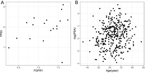
As an illustration of our approach, we tested $H_0:{\rho }_s=0$ versus $H_1:{\rho }_s>0$ using The Cancer Genome Atlas (TCGA) breast cancer RNA sequencing (RNA-seq) data. The gene abundance was RSEM normalized (Li and Dewey 2011). Fibroblast growth factor (FGF)2, FGF4, FGF7 and FGF20 are representative paracrine FGFs binding to heparan-sulfate proteoglycan and fibroblast growth factor receptors (FGFRs), whereas FGF19, FGF21 and FGF23 are endocrine FGFs binding to Klotho and FGFRs. FGFR1 is relatively frequently amplified and overexpressed in breast and lung cancer, and FGFR2 in gastric cancer. Moreover, FGF2 activates human dermal fibroblasts through transcriptional downregulation of the TP53 gene (Katoh 2016). In this application, we examine whether the transcriptomic abundance of FGFR1 is correlated with that of TP53. To investigate the performance in small sample settings, we selected 18 samples from 17 mucinous carcinoma patients. The scatter plot of log-transformed TP53 and FGFR1 abundances is shown in Figure 3a. The marginal normality of data was examined by Shapiro-Wilk test and the bivariate normality was examined by Henze-Zikler test. The p values of Shapiro-Wilk tests for log-transformed TP53 and FGFR1 abundances are 0.6077 and 0.0644, respectively. The p value of Henze-Zikler test is 0.3478. Although there is no statistical significance, the marginal of FGFR1 abundance likely deviates from normal distribution.

Figure 3. Scatter plot of log-transformed TP53 versus FGFR1 abundance for TCGA data (a), and age versus $-\hspace{0.17em}\text{log}\hspace{0.17em}(\text{PSA})$ for the PSA data (b).

The estimated Spearman’s correlation is ${\widehat{\rho }}_s=0.4056.$ Table 3 shows the results of hypothesis testing. Only the result of studentized permutation test is non-significant at $\alpha =0.05$ and suggests there is no evidence of positive correlation between TP53 and FGFR1. In fact the biology does not support a positive correlation either, since FGFR1 mediates negative regulation of TP53 by FGF2 at transcriptional level (Katoh 2016). Indeed, if we include all samples ($n\approx 1200$) from TCGA breast cancer cohort, then all tests will fail to reject H₁ with p-values over 0.5 except for Fisher-Yates test. Together with the results from the simulations, the result by studentized permutation test is clearly more reliable.

Table 3. Results of testing $H_0:{\rho }_s=0$ versus $H_1:{\rho }_s>0$ for TCGA breast cancer data and PSA data.

Tests	p value (TCGA)	p value (PSA)
t test	0.047	< 0.001
Fisher’s Z	< 0.001	< 0.001
Fisher-Yates	< 0.001	< 0.001
Asymp Norm	0.039	< 0.001
Permute	0.033	< 0.001
Stu Permute	0.081	< 0.001

4.2. PSA data

The testing methods were also applied to a data set of age and baseline prostate-specific antigen (PSA) levels (Sweeney et al., 2015). The data consists of age and PSA levels of 480 subjects, of which 473 have complete paired observations. The sample Spearman’s correlation coefficient between age and PSA is ${\widehat{\rho }}_s=-0.1622.$ Since the alternative hypothesis of proposed test is $H_1:{\rho }_s>0,$ we applied a negative log transformation on PSA levels. Similar as the TCGA example, the marginal normality of data was examined by Shapiro-Wilk test, and the bivariate normality was examined by Henze-Zikler test. The p values of Shapiro-Wilk tests for log-transformed age and PSA levels are 0.0208 and 0.0301, respectively. The p value of Henze-Zikler test is < 0.0001. The results indicates the distribution is not bivariate normal. Figure 3b shows the scatter plot of age versus $-\hspace{0.17em}\text{log}\hspace{0.17em}(\text{PSA}).$ Table 3 shows that all tests reject the H₀ and conclude there is a non-zero correlation between age and PSA. The is an example where all tests have consistent results when there is a true correlation. Although the normality tests are significant, such deviation may have been remedied by using the ranks in this specific example.

5. Discussion

Conventional tests of the Spearman’s correlation rely on normality assumption, including t test, Fisher’s Z transformation, and naive permutation test, which fails to control Type I error rates when the assumption is violated. This was illustrated in our simulations studies (Section 3). Such defect cannot be remedied by transforming the marginal distributions such as by Fisher-Yates coefficient. Notably, the deviation from bivariate normality can result in a convergence of type I error rate to an arbitrary level when $n\to \infty .$ This indicates that, under scenarios when two random variables are uncorrelated but dependent, the type I error will not be controlled at desired level no matter how large the sample size is. On the other hand, Serfling’s test based on the delta method guarantees that the type I error rate converges to α as long as the fourth order moment is finite. However, it typically suffers an inflated type I error when sample size is under 50. It should be noted that although we only examined Spearman’s correlation, a similar phenomenon is expected for other rank-based correlation as well, such as Kendall’s τ. The tests based on large sample theories are also anticipated to have inflated type I error when the sample size is small.

We present a robust Spearman’s correlation permutation test based on studentized statistic for testing $H_0:{\rho }_s=0$ versus $H_1:{\rho }_s>0.$ The proposed approach is inspired by the work by DiCiccio and Romano (DiCiccio and Romano 2017), which was developed for Pearson’s correlation. Through extensive simulation studies and real world application, we show the proposed test controls type I error even when sample size is as small as 10 and normality assumption is violated. Therefore, the test is valid in testing monotonic correlations under more general scenarios of underlying distributions and sample sizes. In addition, the studentized statistic can also be used for bootstrapping tests, so as to test for more general point null hypotheses (Hutson 2019). In conclusion, the proposed studentized permutation test should be used as a routine for testing non-zero Spearman’s correlation coefficient.

Acknowledgements

The results shown here are in part based upon data generated by the TCGA Research Network: https://www.cancer.gov/tcga. The PSA data example is based on research using information obtained from www.projectdatasphere.org, which is maintained by Project Data Sphere, LLC. Neither Project Data Sphere, LLC nor the owner(s) of any information from the website have contributed to, approved or are in any way responsible for the contents of this publication.

Additional information

Funding

This work was supported by Roswell Park Cancer Institute and National Cancer Institute (NCI) grant P30CA016056, NRG Oncology Statistical and Data Management Center grant U10CA180822 and IOTN Moonshot grant U24CA232979-01.

References

- Arboretti, R., S. Bonnini, L. Corain, and L. Salmaso. 2014. A permutation approach for ranking of multivariate populations. Journal of Multivariate Analysis 132:39–57. doi:10.1016/j.jmva.2014.07.009.
- Arboretti Giancristofaro, R., S. Bonnini, and F. Pesarin. 2009. A permutation approach for testing heterogeneity in two-sample categorical variables. Statistics and Computing 19 (2):209–16. doi:10.1007/s11222-008-9085-8.
- Basso, D, and L. Salmaso. 2011. A permutation test for umbrella alternatives. Statistics and Computing 21 (1):45–54. doi:10.1007/s11222-009-9145-8.
- DiCiccio, C. J, and J. P. Romano. 2017. Robust permutation tests for correlation and regression coefficients. Journal of the American Statistical Association 112 (519):1211–20. doi:10.1080/01621459.2016.1202117.
- Edgell, S. E, and S. M. Noon. 1984. Effect of violation of normality on the t test of the correlation coefficient. Psychological Bulletin 95 (3):576–83. doi:10.1037/0033-2909.95.3.576.
- Fieller, E. C., H. O. Hartley, and E. S. Pearson. 1957. Tests for rank correlation coefficients. I. Biometrika 44 (3-4):470–81. doi:10.1093/biomet/44.3-4.470.
- Fisher, R. A, and F. Yates. 1938. Statistical tables: For biological, agricultural and medical research. Edinburgh, United Kingdom:Oliver and Boyd.
- Giancristofaro, R. A. 2014. Permutation solutions for multivariate ranking and testing with applications. Communications in Statistics – Theory and Methods 43 (4):891–905. doi:10.1080/03610926.2013.802808.
- Giancristofaro, R. A, and S. Bonnini. 2008. Moment-based multivariate permutation tests for ordinal categorical data. Journal of Nonparametric Statistics 20 (5):383–93. doi:10.1080/10485250802195440.
- Hutson, A. D. 2019. A robust Pearson correlation test for a general point null using a surrogate bootstrap distribution. PLoS One 14 (5):e0216287.
- Hutson, A. D, and H. Yu. 2021. A robust permutation test for the concordance correlation coefficient. Pharmaceutical Statistics 20 (4):696–709. doi:10.1002/pst.2101.
- Katoh, M. 2016. FGFR inhibitors: Effects on cancer cells, tumor microenvironment and whole-body homeostasis. International Journal of Molecular Medicine 38 (1):3–15. doi:10.3892/ijmm.2016.2620.
- Kendall, M, and A. Stuart. 1979. Vol. 2 of The advanced theory of statistics, 240–80. London: Charles Griffin.
- Li, B, and C. N. Dewey. 2011. RSEM: Accurate transcript quantification from RNA-Seq data with or without a reference genome. BMC Bioinformatics 12 (1):323. doi:10.1186/1471-2105-12-323.
- Marozzi, M. 2014. Testing for concordance between several criteria. Journal of Statistical Computation and Simulation 84 (9):1843–50. doi:10.1080/00949655.2013.766189.
- Moran, P. 1948. Rank correlation and product-moment correlation. Biometrika 35 (Pts 1-2):203–6.
- Pauly, M, and L. Smaga. 2020. Asymptotic permutation tests for coefficients of variation and standardised means in general one-way ANOVA models. Statistical Methods in Medical Research 29 (9):2733–48. doi:10.1177/0962280220909959.
- Pearson, K. 1896. VII. Mathematical contributions to the theory of evolution.—III. Regression, heredity, and panmixia. Philosophical Transactions of the Royal Society of London. Series A, Containing Papers of a Mathematical or Physical Character (187):253–318.
- Pesarin, F, and L. Salmaso. 2010a. Finite-sample consistency of combination-based permutation tests with application to repeated measures designs. Journal of Nonparametric Statistics 22 (5):669–84. doi:10.1080/10485250902807407.
- Pesarin, F, and L. Salmaso. 2010b. The permutation testing approach: A review. Statistica 70 (4):481–509.
- Pesarin, F, and L. Salmaso. 2012. A review and some new results on permutation testing for multivariate problems. Statistics and Computing 22 (2):639–46. doi:10.1007/s11222-011-9261-0.
- Pesarin, F, and L. Salmaso. 2013. On the weak consistency of permutation tests. Communications in Statistics - Simulation and Computation 42 (6):1368–79. doi:10.1080/03610918.2012.625338.
- R Core Team. 2013. R: A Language and Environment for Statistical Computing. Vienna, Austria: R Foundation for Statistical Computing.
- Salmaso, L. 2015. Combination-based permutation tests: Equipower property and power behavior in presence of correlation. Communications in Statistics - Theory and Methods 44 (24):5225–39. doi:10.1080/03610926.2013.810270.
- Salmaso, L, and F. Pesarin. 2010. Permutation tests for complex data: Theory, applications and software. Chichester, United Kingdom: John Wiley & Sons.
- SAS Institute 2015. Base SAS 9.4 procedures guide. Cary, NC, U.S.:SAS Institute.
- Spearman, C. 1961. The proof and measurement of association between two things. In Studies in individual differences: The search for intelligence, ed., J. J. Jenkins and D. G. Paterson, (pp. 45–58). New York, NY, U.S.: Appleton-Century-Crofts.
- Stanton, J. M. 2001. Galton, Pearson, and the peas: A brief history of linear regression for statistics instructors. Journal of Statistics Education 9 (3):1–13. doi:10.1080/10691898.2001.11910537.
- Sweeney, C. J., Y.-H. Chen, M. Carducci, G. Liu, D. F. Jarrard, M. Eisenberger, Y.-N. Wong, N. Hahn, M. Kohli, M. M. Cooney, et al. 2015. Chemohormonal therapy in metastatic hormone-sensitive prostate cancer. New England Journal of Medicine 373 (8):737–46. doi:10.1056/NEJMoa1503747.