On the Conway-Maxwell-Poisson point process

Abstract

The Poisson point process plays a pivotal role in modeling spatial point patterns. One of its key features is that the variance and the mean of the total number of points in a given region are equal, making it unsuitable for modeling point patterns that exhibit significantly different mean and variance. To tackle such point patterns, we introduce the class of Conway-Maxwell-Poisson point processes. Our model can easily be fitted with a logistic regression, its point counts in different regions are correlated and its log-likelihood in any subregion can be easily extracted. Both simulations and real data analyses have been carried out to demonstrate the performance of the proposed model.

KEYWORDS:

• Spatial point process
• replicated point pattern
• Conway-Maxwell-Poisson distribution
• Papangelou conditional intensity
• bootstrap

1 Introduction

As the cornerstone of spatial point processes, the Inhomogeneous Poisson Process (IPP) plays a pivotal role in modeling spatial point patterns in a wide range of research areas such as forestry and plant ecology (Thompson 1955), astronomy (Babu and Feigelson 1996), epidemiology (Waller and Gotway 2004), geology (Connor and Hill 1995), and wireless networks (Andrews et al. 2010). The IPP consists of a Poisson number of independent and identically distributed (iid) points over a bounded observation region, hence, by assumption, it has two features: the mean and variance of the total count in any subregion are equal (equi-dispersion) and the counts of points in disjoint subregions are independent. In real-world applications, few point patterns exhibit both of these features. When the variance-to-mean ratio is greater than one, the negative binomial point process discussed in Diggle and Milne (1983) can be used but there are few choices of models that can handle point patterns with all possible variance-to-mean ratios.

To model count data, Conway and Maxwell (1962) proposed a Conway-Maxwell Poisson (CMP) distribution that is capable of accommodating both overdispersion (variance-to-mean ratio bigger than one) and underdispersion (variance-to-mean ratio smaller than one). In contrast to the equi-dispersion feature of the Poisson distribution, the CMP distribution includes an extra parameter controlling dispersion which can be tailored to meet the variance-to-mean ratio of the count data. The CMP distribution has also been proposed as a generalization of the Poisson distribution in the context of generalized linear model regressions (Sellers and Shmueli, 2010), yielding a wide range of applications. A comprehensive overview regarding the CMP model was provided by Sellers, Borle, and Shmueli (2012). MacDonald and Bhamani (2020), Alqawba and Diawara (2021), Zhu (2012), and Melo and Alencar (2020) extended the CMP to new classes of time series models of count data that is equidispersed, underdispersed, and/or overdispersed. Wu, Holan, and Wikle (2013) modeled spatiotemporal count data using multivariate conditionally independent CMP distributions with intensity process governed by a dynamical spatiotemporal process. Li and Dey (2022) proposed a similar model of COVID-19 mortality in given states in terms of spatial and temporal covariates. All these work have in common that they model aggregated count data, whether it is counts over time or spatiotemporal counts. In contrast, in this work, we will extend the CMP distribution to a CMP point process which can be used to model spatiotemporal point pattern data.

Previous research has attempted to develop a point process model such that the total number of point counts within any given interval follows the CMP distribution, and has stationary and independent increments. Zhu et al. (2017) proposed a homogeneous counting process on the real line by specifying that the numbers of events within unit intervals $(t,t+1]$ for $t=0,1,2,\dots$ are independent and follow the CMP distribution. However, Proposition 1 in Appendix proves that the CMP process in Zhu et al. (2017)’s work cannot exist unless it is a homogeneous Poisson process. To remedy the problem faced by Zhu et al. (2017), we develop a class of CMP processes ($\text{CMPP}$) that can model random point patterns in both space and time. Moreover, our model accommodates homogeneous or inhomogeneous intensity that are dependent on space and time, in contrast to the strictly time-homogeneous framework of Zhu et al. (2017). We also introduce a quick and reliable inference procedure that eliminates the need for computation the challenging normalizing constant present in the CMP’s probability mass function. Compared to the spatiotemporal CMP models that divide the space into cells and regress the cell counts in Wu, Holan, and Wikle (2013), our $\text{CMPP}$ models the rate of occurrence of events directly, without aggregation, by treating the data as arising from a point process. The $\text{CMPP}$ also caters for dependence between the counts of points in disjoint subregions (see Proposition 2) and it is easy to extract the likelihood for the point patterns restricted to any subregion in order to make inference on subregions of interest (see Proposition 3). In case studies, we demonstrate that the CMP process serves as a solid model of replicated spatial point patterns, which are commonly observed in practice (Chapter 16 of Baddeley et al. 2014).

The article is organized as follows. In Section 2, we elaborate on the definition of the $\text{CMPP}$ and set up its inference procedure. In Section 3, numerical simulations are carried out to demonstrate its performance. To illustrate its applications, we apply the new point process in Section 4 to the analysis of daily bike trips data in Chicago, to sightings of the wildflower Arctotheca calendula in South-East Australia, as well as to records of flooding in the Rio Negro river. The article concludes with a discussion in Section 5.

2 Methodology and inference

2.1 Methodology

Conway and Maxwell (1962) defined a CMP distribution by its probability mass function (1) $$f(i)=\frac{{\lambda }^i}{Z(\lambda ,\nu ){(i!)}^{\nu }},\hspace{1em}i\in {\mathbb{Z}}_{+}:=\{0,1,2,\dots \},$$(1) where $\lambda ,\nu \ge 0$ are parameters, and $Z(\lambda ,\nu )$ is the normalizing constant. The level of dispersion can be conveniently characterized by the dispersion parameter ν, with ν = 1, $\nu <1$, and $\nu >1$ corresponding to equi-dispersion (i.e., the Poisson distribution), overdispersion, and underdispersion, respectively. The CMP distribution is thus more flexible than the Poisson distribution in capturing complex behaviors exhibited by count data in applications (Sellers, Borle, and Shmueli 2012; Mannering and Bhat 2014).

General spatial point processes in a region W can be generated by first drawing the number of points N from a probability mass function (hereafter, pmf) f on ${\mathbb{Z}}_{+}$. Then, conditional on N = n, the point patterns are sampled according to a conditional probability density function $h(\{x_1,\dots ,x_n\left\}\right|n)$ on W (see Kroese and Botev 2015 and Proposition 5.3.II in Daley and Vere-Jones 2003). For a given probability density function (hereafter, pdf) μ on W, an IPP on W is obtained if $f(i)={\lambda }^i\hspace{0.17em}\exp \hspace{0.17em}(-\lambda )/i!$ (i.e., f a Poisson pmf with mean λ) and points are drawn independently according to μ. The intensity of the IPP, defined as $\Lambda :=\mu \lambda$, represents the average number of points per unit area. As some of the more remarkable properties of an IPP, the number of points that fall in a set $A\subset W$ is again Poisson distributed and the numbers of points in disjoint sets $A,B\subset W$ are independent.

Here we propose a class of Conway-Maxwell-Poisson processes (hereafter, CMPP) by taking f as the CMP pmf (1)(1) $$f(i)=\frac{{\lambda }^i}{Z(\lambda ,\nu ){(i!)}^{\nu }},\hspace{1em}i\in {\mathbb{Z}}_{+}:=\{0,1,2,\dots \},$$(1) with parameters $\lambda ,\nu \ge 0$ and, just as in the IPP setting, drawing points on W independently with pdf μ. Thus, in this more general case, there are two real parameters λ and ν and one functional parameter μ. As in the IPP setting, we set $\Lambda :=\lambda \mu$ in our proposed model. However, it is important to note that Λ is in general not the intensity of CMPP, that is, the average number of points per unit area, since λ is in general not the mean of the CMP distribution. We shall delve into this in more detail later on.

This leads us to calling Λ a quasi-intensity function (see Proposition 4 in Appendix for a computation of the intensity). It is easy to check that our proposed $\text{CMPP}$ is completely parametrized by ν and the function Λ (indeed, the first parameter of the CMP is obtained by integrating both sides of the equation defining Λ over W, yielding $\lambda =\mathcal{l}(\Lambda ):={\int }_W\Lambda (x) \mathrm{d}x$, and the conditional pdf of the points is obtained as $\mu =\Lambda /\mathcal{l}(\Lambda )$). A $\text{CMPP}$ is therefore denoted by $\text{CMPP}(\Lambda ,\nu )$. We observe that the average total number of points in a $\text{CMPP}(\Lambda ,\nu )$ is not in general $\mathcal{l}(\Lambda )$, but is the mean of the CMP distribution with parameters $\mathcal{l}(\Lambda )$ and ν, which does not in general have a closed form.

In summary, we draw samples of a $\text{CMPP}(\Lambda ,\nu )$, with dispersion parameter ν and quasi-intensity function Λ, in the following two steps:

1. generate the total number of points N from a CMP distribution with parameters $\lambda =\mathcal{l}(\Lambda )$ and ν;

2. given the observed value N = n, draw n points independently with pdf $\mu =\Lambda /\mathcal{l}(\Lambda )$.

Remark 1.

(i) The IPP is a special case of the $\text{CMPP}(\Lambda ,\nu )$ in which ν = 1. (ii) If Λ is a constant and W is an interval, then the $\text{CMPP}(\Lambda ,\nu )$ has stationary (but in general non independent) increments, achieves the goal of Zhu et al. (2017) and is tractable. (iii) The $\text{CMPP}(\Lambda ,\nu )$ point process can be used to model either positive or negative correlation between the counts falling into two disjoint regions; see Proposition 2 in Appendix. The correlation becomes zero when ν = 1, which is a consequence of point (i) above, namely that the $\text{CMPP}(\Lambda ,1)$ reduces to the IPP model.

The quasi-intensity function Λ in practice is assumed to be influenced by spatial or environmental covariates $\mathit{x}(s)$, such as elevation, temperature, or rainfall at a location s. A common way to model $\Lambda (s)$ is through a log-linear model (2) $$\hspace{0.17em}\ln \hspace{0.17em}(\Lambda (s))={\beta }_0+\sum _{j=1}^m{\beta }_j{x}_j(s),$$(2) where ${\mathit{x}}^T(s):=(1,x_1(s),\dots ,x_m(s))$ and the vector ${\mathit{\beta }}^T:=({\beta }_0,{\beta }_1,\dots ,{\beta }_m)$ is the regression coefficient for the corresponding covariates. The quasi-intensity Λ governs how the spatial points are distributed, and is also associated with the pmf f via $\lambda =\mathcal{l}(\Lambda )$ in our definition. This latter property in particular means that, all else being equal, the larger the quasi-intensity, the higher the average number of points. The log-linear modeling of the quasi-intensity indirectly affects the average total count modeling since $$\lambda ={\int }_W\Lambda (s) \mathrm{d}s,$$ which reduces to a log-linear model on λ if the spatial covariates are constant. Some of the more recent literature has considered other link functions, see, for example, Ribeiro et al. (2020), Huang (2017), and Weiss, Zhu, and Hoshiyar (2020). In any case, a log-linear model of λ was found to be useful and have reasonable properties in Sellers, Borle, and Shmueli (2012).

The Janossy intensity of the point process (Daley and Vere-Jones 2003, Section 5.3) is the function j such that $$j(\{x_1,\dots ,x_n\}) \mathrm{d}{x}_1\cdots \mathrm{d}{x}_n$$is the probability that there are n points around $x_1,\dots ,x_n$. In point process theory, this function plays a role analogous to that of the probability density function of a random variable. It can be shown that the proposed point process has Janossy density given by (3) $$j(\{x_1,\dots ,x_n\})=\frac{1}{Z(\mathcal{l}(\Lambda ),\nu ){(n!)}^{\nu -1}}\prod _{i=1}^n\Lambda (x_i),\hspace{1em}\{x_1,\dots ,x_n\}\subset W.$$(3)

Denoting the mean of f by $\mathbb{E}[N]$, we show in Proposition 4 that the true intensity function ϱ of the $\text{CMPP}(\Lambda ,\nu )$ is given by $$\varrho (x)=\Lambda (x)\frac{\mathbb{E}\left[N\right]}{\mathcal{l}(\Lambda )}.$$

The quasi-intensity function Λ equals the true intensity function ϱ if and only if $\mathbb{E}[N]=\mathcal{l}(\Lambda )$, that is, N is a Poisson random variable.

2.2 Inference

In practice, we shall make inference on K > 1 independent samples, where each sample is a $\text{CMPP}({\Lambda }^{(k)},\nu )$ with fixed dispersion parameter ν and sample varying intensity given by (4) $$\hspace{0.17em}\ln \hspace{0.17em}({\Lambda }^{(k)}(s))={\beta }_0+\sum _{j=1}^m{\beta }_j{x}_j^{(k)}(s),\hspace{1em}k=1,\dots ,K,$$(4) for a unique sample-independent $\mathit{\beta }$. The sample-varying intensity allows us in practice to accommodate sample-dependent (for example time-varying) covariates. We use $\{z_1^{(k)},\dots ,z_{n_k}^{(k)}\}$ to denote the data corresponding to the k-th sample of the point process. From (3)(3) $$j(\{x_1,\dots ,x_n\})=\frac{1}{Z(\mathcal{l}(\Lambda ),\nu ){(n!)}^{\nu -1}}\prod _{i=1}^n\Lambda (x_i),\hspace{1em}\{x_1,\dots ,x_n\}\subset W.$$(3) , the log-likelihood of K independent samples is (5) $$-(\nu -1)\sum _{k=1}^K\hspace{0.17em}\ln \hspace{0.17em}(n_k!)-\sum _{k=1}^K\hspace{0.17em}\ln \hspace{0.17em}(Z(\mathcal{l}({\Lambda }^{(k)}),\nu ))+\sum _{k=1}^K\sum _{i=1}^{n_k}\hspace{0.17em}\ln \hspace{0.17em}({\Lambda }^{(k)}(z_i^{(k)})).$$(5)

Although the log-likelihood given by (5)(5) $$-(\nu -1)\sum _{k=1}^K\hspace{0.17em}\ln \hspace{0.17em}(n_k!)-\sum _{k=1}^K\hspace{0.17em}\ln \hspace{0.17em}(Z(\mathcal{l}({\Lambda }^{(k)}),\nu ))+\sum _{k=1}^K\sum _{i=1}^{n_k}\hspace{0.17em}\ln \hspace{0.17em}({\Lambda }^{(k)}(z_i^{(k)})).$$(5) allows us to estimate the unknown parameters $\mathit{\beta }$ and ν, the intractable constants $\hspace{0.17em}\ln \hspace{0.17em}(Z(\mathcal{l}({\Lambda }^{(k)}),\nu ))$ render it an impractical way to make statistical inference. A wide range of inference techniques have been developed in the statistical point process literature. We shall use the technique developed in Baddeley et al. (2014) to estimate $\mathit{\beta }$ and ν.

The method of Baddeley et al. (2014) hinges on the Papangelou conditional intensity π of the point process (Daley and Vere-Jones 2008, Definition 10.4.I). In short, the Papangelou conditional intensity π is a function such that $\pi (z,\{z_1,\dots ,z_n\}) \mathrm{d}z$ is the probability that there is a point around a location z conditional on the configuration $\{z_1,\dots ,z_n\}$ (outside of $\mathrm{d}z$). Contrary to the Janossy intensity, the Papangelou conditional intensity gives information on the conditional probability of finding new individuals, given an existing configuration. The Papangelou conditional intensity of our point process is given by (6) $$\begin{array}{c}\pi (z,\{z_1,\dots ,z_n\}):=\frac{j(\{z_1,\dots ,z_n\}\cup \{z\})}{j(\{z_1,\dots ,z_n\}\setminus \{z\})}\\ =\frac{\Lambda (z)}{{(n+{\mathbf{1}}_{\{z\notin \{z_1,\dots ,z_n\left\}\right\}})}^{\nu -1}}\\ =\hspace{0.17em}\exp \hspace{0.17em}(\hspace{0.17em}\ln \hspace{0.17em}(\Lambda (z))+(1-\nu )\hspace{0.17em}\ln \hspace{0.17em}(n+{\mathbf{1}}_{\{z\notin \{z_1,\dots ,z_n\left\}\right\}})),\end{array}$$(6) where ${\mathbf{1}}_A$ stands for the indicator function of a set A. By assuming the log-linear form for $\Lambda (s)$ in (2)(2) $$\hspace{0.17em}\ln \hspace{0.17em}(\Lambda (s))={\beta }_0+\sum _{j=1}^m{\beta }_j{x}_j(s),$$(2) , the Papangelou conditional intensity π can now be written in the form of (7) $$\pi (z,\{z_1,\dots ,z_n\})=\hspace{0.17em}\exp \hspace{0.17em}({\mathit{\theta }}^T\mathit{t}(z,\{z_1,\dots ,z_n\}\backslash \left\{z\right\})),$$(7)

for a vector of parameters $\mathit{\theta }$ and a function t, with ${\mathit{\theta }}^T=({\mathit{\beta }}^T,1-\nu )$ and (8) $${\mathit{t}}^T(z,\{z_1,\dots ,z_n\}\setminus \{z\})=(1,x_1(z),\dots ,x_m(z),\hspace{0.17em}\ln \hspace{0.17em}({\mathbf{1}}_{\{z\notin \{z_1,\dots ,z_n\left\}\right\}}+n)).$$(8)

Baddeley et al. (2014) imply that, given the log-exponential form (8)(8) $${\mathit{t}}^T(z,\{z_1,\dots ,z_n\}\setminus \{z\})=(1,x_1(z),\dots ,x_m(z),\hspace{0.17em}\ln \hspace{0.17em}({\mathbf{1}}_{\{z\notin \{z_1,\dots ,z_n\left\}\right\}}+n)).$$(8) , inference can be done by running a logistic regression with an offset term. Using point process fitting software, it suffices to run the logistic regression with an additional artificial covariate with value $\hspace{0.17em}\ln \hspace{0.17em}({\mathbf{1}}_{\{z\notin \{z_1,\dots ,z_n\left\}\right\}}+n)$. This is particularly easy to do by using the spatstat (Baddeley, Rubak, and Turner 2015) package in the R programming language. Since the technique developed in Baddeley et al. (2014) is based on a logistic regression, it is straightforward to generalize it to independent point process samples with log-likelihood (5)(5) $$-(\nu -1)\sum _{k=1}^K\hspace{0.17em}\ln \hspace{0.17em}(n_k!)-\sum _{k=1}^K\hspace{0.17em}\ln \hspace{0.17em}(Z(\mathcal{l}({\Lambda }^{(k)}),\nu ))+\sum _{k=1}^K\sum _{i=1}^{n_k}\hspace{0.17em}\ln \hspace{0.17em}({\Lambda }^{(k)}(z_i^{(k)})).$$(5) .

In addition, we summarize the key points to implement the logistic regression for the proposed $\text{CMPP}(\Lambda ,\nu )$ by hand as follows.

1. Generate m dummy points, say $\{y_1,\dots ,y_m\}$, independently from the sample, where m is a realization of a random variable with known mean M.

2. Compute $\mathit{t}(z,\{z_1^{(k)},\dots ,z_{n_k}^{(k)}\}\setminus \{z\})$ as z ranges over the points in the configuration $\{z_1^{(k)},\dots ,z_{n_k}^{(k)}\}\cup \{y_1,\dots ,y_m\}$ and k ranges in $\{1,\dots ,K\}$, where t has been defined in (8)(8) $${\mathit{t}}^T(z,\{z_1,\dots ,z_n\}\setminus \{z\})=(1,x_1(z),\dots ,x_m(z),\hspace{0.17em}\ln \hspace{0.17em}({\mathbf{1}}_{\{z\notin \{z_1,\dots ,z_n\left\}\right\}}+n)).$$(8) . This yields a regression matrix with ${\sum }_{k=1}^K(n_k+m)$ observations, and m + 2 regressors.

3. Estimate the unknown parameter ${\mathit{\theta }}^T=({\mathit{\beta }}^T,1-\nu )$ by a logistic regression with response 1 for the observed points and 0 for the dummy points, input variable t computed above, and offset term $-\hspace{0.17em}\ln \hspace{0.17em}(M/|W|)$. (We refer to Baddeley et al. 2014 for more details on why this offset term appears.)

In order to set up the logistic regression, we have used the spatstat (Baddeley, Rubak, and Turner 2015) package in R. When estimating parameters of the $\text{CMPP}(\Lambda ,\nu )$, we have reported parametric bootstrap confidence intervals which have been considered for example in Section 8.3 of Baddeley and Turner (2000). Asymptotic confidence intervals can also be estimated by the technique introduced in Coeurjolly and Rubak (2013) (see also Section 4 and the appendices of Baddeley et al. 2014). These latter confidence intervals have been reported when doing inference for the IPP.

3 Numerical simulations

In this section, we demonstrate the performance of the $\text{CMPP}$ on simulated datasets. The numerical studies have been carried out using the R language (R Core Team, 2019). The CMP random variables were simulated using the COMPoissonReg package in R (based on Minka et al. 2002) and the logistic regression was implemented via the spatstat package in R. In all the numerical simulations, we have used 1, 000 dummy points when implementing the inference method of Section 2.2.

3.1 Homogeneous study

We consider 200 iid distributed samples from a $\text{CMPP}(\Lambda ,\nu )$ distribution with constant quasi-intensity Λ and dispersion parameter ν on an observation window $W={[0,1]}^2$. Since in this simple case there is no spatial inhomogeneity, a CMP model on the total point counts would yield similar results. We study R = 200 independent replications of this iid sequence, so that we draw $200\times 200=40,000$ samples from the $\text{CMPP}(\Lambda ,\nu )$ distribution in total. For each of the R replications, we construct an estimate $(\widehat{\hspace{0.17em}\ln \hspace{0.17em}(\Lambda )},\widehat{\nu })$ by our inference method. We then compute the 95% bootstrap confidence intervals by sampling N_b = 500 draws from the fitted model, with parameters $(\widehat{\hspace{0.17em}\ln \hspace{0.17em}(\Lambda )},\widehat{\nu })$. Our focus is then on the mean parameter estimates, obtained by averaging the estimates over the R replications, and the coverage probabilities, that is, the proportion of confidence intervals which contain the true values of the parameters.

In the following analysis, we consider six different pairs of parameters $(\hspace{0.17em}\ln \hspace{0.17em}(\Lambda ),\nu )$: $(1.15,0.5),(2.30,1),(4.61,2),(0.347,0.5),(0.693,1)$, and $(1.39,2)$. These values of ν are chosen to represent a range of different dispersions, and $\hspace{0.17em}\ln \hspace{0.17em}(\Lambda )$ is chosen so that in each sample the average number of points is 10 for the first three pairs of values, and 2 for the remaining three pairs. The results of our analysis are shown in Table 1, where the mean estimates of the parameters and the coverage probabilities are provided. We see in Table 1 that the mean estimates and coverage probabilities are reasonably accurate. The coverage probability does not always reach the expected 95%, especially when $\nu <1$ or when point count is low, perhaps due to limitations of our bootstrapping method.

Table 1 Estimates of parameters for the homogeneous study.

Parameter	True value	Mean estimate	Coverage probability
$\hspace{0.17em}\ln \hspace{0.17em}(\Lambda )$	1.15	1.20	0.90
ν	0.5	0.519	0.91
$\hspace{0.17em}\ln \hspace{0.17em}(\Lambda )$	2.30	2.35	0.95
ν	1	1.02	0.94
$\hspace{0.17em}\ln \hspace{0.17em}(\Lambda )$	4.61	4.72	0.95
ν	2	2.05	0.96
$\hspace{0.17em}\ln \hspace{0.17em}(\lambda )$	0.347	0.366	0.91
ν	0.5	0.521	0.94
$\hspace{0.17em}\ln \hspace{0.17em}(\lambda )$	0.693	0.709	0.93
ν	1	1.02	0.92
$\hspace{0.17em}\ln \hspace{0.17em}(\lambda )$	1.39	1.42	0.93
ν	2	2.04	0.91

We now focus on one set of values, $(\hspace{0.17em}\ln \hspace{0.17em}(\Lambda ),\nu )=(1.15,0.5)$ and we consider some properties of the joint estimator. We produce R = 200 simulated replications, each containing 200 iid samples of a $\text{CMPP}(\hspace{0.17em}\exp \hspace{0.17em}(1.15),0.5)$ on an observation window $W={[0,1]}^2$. In each of the R replications, we estimate the unknown parameters $\hspace{0.17em}\ln \hspace{0.17em}(\Lambda )$ and ν according to the inference method described in Section 2.1. The resulting pairs of estimates $(\widehat{\hspace{0.17em}\ln \hspace{0.17em}(\Lambda )},\widehat{\nu })$ are then plotted on the left-hand side of Figure 1. We find that estimates of $\hspace{0.17em}\ln \hspace{0.17em}(\Lambda )$ and ν are linearly associated.

Fig. 1 Left-hand side: Distribution of estimates $(\widehat{\hspace{0.17em}\ln \hspace{0.17em}(\Lambda )},\widehat{\nu })$. The true value is $(1.15,0.5)$. Right-hand side: Contour plot of the estimation of the mean of a CMP distribution (for 10, 000 Monte-Carlo draws), for different values of Λ and ν.

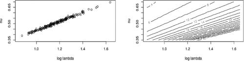
This linear association was found in Zhu et al. (2017) and partly justifies a reparametrization of the CMP proposed in Ribeiro et al. (2020). In order to further illustrate this linear association, we show a contour plot on the right-hand side of Figure 1 of estimates of the mean of a CMP distribution for values around $(\hspace{0.17em}\ln \hspace{0.17em}(\Lambda ),\nu )=(1.15,0.5)$. We observe that in this range, the mean of a CMP distribution is increasing in Λ and decreasing in ν. Hence, for a given estimate of the mean, a large estimate of Λ would coincide with a large estimate of ν. Indeed, we find that the values of our estimator $(\widehat{\hspace{0.17em}\ln \hspace{0.17em}(\Lambda )},\widehat{\nu })$ are distributed around the curve corresponding to the sample mean 10.

3.2 Inhomogeneous study

In this section, we consider a sequence of independent inhomogeneous samples, coming from a $\text{CMPP}({\Lambda }^{(k)},\nu )$, where ${\Lambda }^{(k)}(s)$ depends on a spatiotemporal covariate $x^{(k)}(s)$ at location $s\in W={[0,1]}^2$ according to (9) $${\Lambda }^{(k)}(s)=\hspace{0.17em}\exp \hspace{0.17em}({\beta }_0+\beta x^{(k)}(s)).$$(9)

Here β₀ is the intercept, β is the regression coefficient, and $x^{(k)}(s)$ represents a seasonally varying temperature gradient defined as $$x^{(k)}(s)=y(s)+\hspace{0.17em}\cos \hspace{0.17em}\left(\frac{2\pi k}{50}\right),$$with y(s) the y-coordinate of location s. The true parameter values are given by $({\beta }_0,\nu ,\beta )=(1.5,0.8,2.5)$. We have also considered a collection of 50 independent samples, and R = 100 replications have been used in the simulation. The point locations distributed according to (9)(9) $${\Lambda }^{(k)}(s)=\hspace{0.17em}\exp \hspace{0.17em}({\beta }_0+\beta x^{(k)}(s)).$$(9) have been drawn by rejection sampling. Similarly to the analysis carried out in the previous section, we construct mean parameter estimates, along with coverage probabilities associated with parametric bootstrap confidence intervals with N_b = 200 bootstrap samples. The results are presented in Table 2.

Table 2 Estimates of parameters for the inhomogeneous study.

Parameter	True value	Mean estimate	Coverage probability
β0	1.5	1.52	0.95
ν	0.8	0.808	0.95
β	2.5	2.52	0.92

As in the homogeneous study, the results in Table 2 show that the inference works well for the inhomogeneous case. The mean parameter estimates are particularly close to the true values; this is due to the fact that our temperature covariate varies strongly between samples, allowing for a highly accurate fit.

In order to evaluate its performance on large datasets, we also present in Table 3 the results for the parameters $({\beta }_0,\nu ,\beta )=(4,0.8,2.5)$. This corresponds to an average of more than 5, 000 points per sample, that is, over 500, 000 spatial points in total. We reduced the number of bootstrap replications to N_b = 100 to make the computation time more manageable. The mean parameter estimates and coverage probabilities are excellent. The mean estimates are much more precise than those in Table 2 thanks to the large amount of data used in this case.

Table 3 Estimates of parameters for the inhomogeneous study on a large dataset.

Parameter	True value	Mean estimate	Coverage probability
β0	4.0	4.0007	0.92
ν	0.8	0.8002	0.94
β	2.5	2.5004	0.97

Table 4 Estimate of the Pearson correlation coefficient $\widehat{\rho }$ between point counts in two neighboring subregions.

ν	0.1	0.2	0.3	0.4	0.5
$\widehat{\rho }$	0.587	0.418	0.310	0.232	0.174
CI	(0.585, 0.588)	(0.417,0.420)	(0.308,0.311)	(0.230,0.234)	(0.172, 0.175)
ν	0.6	0.7	0.8	0.9	1.0
$\widehat{\rho }$	0.126	0.087	0.055	0.025	0.0014
CI	(0.124,0.128)	(0.086,0.089)	(0.053,0.057)	(0.023,0.027)	(–0.0006, 0.0034)
ν	1.1	1.2	1.3	1.4	1.5
$\widehat{\rho }$	0.001	–0.041	–0.061	–0.076	–0.092
CI	(–0.025,–0.019)	(–0.043,–0.039)	(–0.063,-0.059)	(–0.078,-0.074)	(–0.094,-0.091)
ν	1.6	1.7	1.8	1.9	2.0
$\widehat{\rho }$	–0.106	–0.118	–0.132	–0.142	–0.152
CI	(–0.108, –0.104)	(–0.120, –0.116)	(–0.134, –0.130)	(–0.144, –0.141)	(–0.154, –0.150)

N.B. The data was generated from a $\text{CMPP}(\Lambda ,\nu )$ model with quasi-intensity Λ = 1 and different values of ν. The observation window $W={[0,1]}^2$ is divided into two neighboring subregions, $W_1=\{(s_1,s_2):s_1\le 0.5\}$ and $W_2=\{(s_1,s_2):s_1>0.5\}$. Pearson correlation coefficients have been computed based on 1,000,000 samples, along with the asymptotic 95% confidence intervals.

3.3 Correlation of point counts

In this subsection, we illustrate point (iii) in Remark 1. We consider a $\text{CMPP}(\Lambda ,\nu )$ point process with quasi-intensity Λ = 1 (constant) and different values of ν on an observation window $W={[0,1]}^2$. We define two different subregions $W_1=\{(s_1,s_2):s_1\le 0.5\}$ and $W_2=\{(s_1,s_2):s_1>0.5\}$. The following table shows the estimates of the Pearson correlation coefficients over 10⁶ samples between point counts in W₁ and W₂ along with the corresponding asymptotic 95% confidence intervals (CI). We clearly observe that point counts are positively correlated when $\nu <1$, negatively correlated when $\nu >1$, and are independent when ν = 1 (recall that this last case corresponds to the Poisson point process).

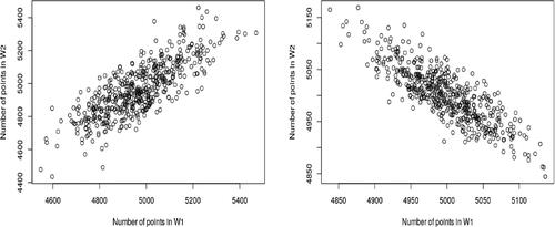
We now illustrate this finding by looking in detail at three possible values for ν, choosing in each case Λ so that the average number of points per sample is equal to 10⁴. In Figure 2, we show the number of counts in two subregions W₁ and W₂ with 500 independent replications of the model. On the left side panel of Figure 2, we choose $\nu <1$, in which case the point counts in W₁ and W₂ are expected to be positively correlated. The two point counts are clearly positively correlated with a 95% CI of $(0.7593,0.8244)$ and we reject the hypothesis of zero correlation with p-value $<2.2·{10}^{-16}$. On the right side panel of Figure 2, instead, we choose $\nu >1$ and the two point counts are clearly negatively correlated (95% confidence interval of $(-0.8569,-0.8025)$ and we reject the hypothesis of zero correlation with p-value $<2.2·{10}^{-16}$).

Fig. 2 Scatter plots of the total number of individuals in two subregions W₁ and W₂ for the $\text{CMPP}(\Lambda ,\nu )$. The left panel shows the result for the parameters $(2.51,0.1)$ with positive relation; the right panel corresponds to $({10}^{40},10)$ with negative relation. The number of replications is 500.

We next consider a Poisson point process with the same average number of points as in the previous two cases of Figure 2, and the scatter plot of the total number of counts in the two regions is given in Figure 3. The 95% CI of the Pearson correlation coefficient for the Poisson process is estimated as $(-0.1259,0.0493)$ (with p-value 0.39), indicating that there is no strong evidence to reject the hypothesis of no correlation between point counts. This confirms that the IPP does not exhibit positive or negative correlation of point counts between different regions as does the $\text{CMPP}(\Lambda ,\nu )$.

Fig. 3 Scatter plots of the total number of individuals in two subregions W₁ and W₂ for the Poisson point process with intensity $\Lambda ={10}^4$. The number of replications is 500.

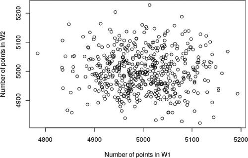
Another feature of these figures is that they show under or over dispersion of point counts compared to the Poisson point process. It can be seen from Figure 2 that when $\nu <1$ the range of point counts in each region is roughly $[4400,5400]$, and the range is about $[4850,5150]$ when $\nu >1$. However in the Poisson case in Figure 3, we observe a range $[4800,5200]$ which is between the two ranges above. In other words, compared to the Poisson point process, point counts are overdispersed when $\nu <1$ and underdispersed when $\nu >1$. This is a characterizing feature of the CMP distribution (1)(1) $$f(i)=\frac{{\lambda }^i}{Z(\lambda ,\nu ){(i!)}^{\nu }},\hspace{1em}i\in {\mathbb{Z}}_{+}:=\{0,1,2,\dots \},$$(1) which drives the number of points of our CMPP.

4 Real case study

In this section, we study three replicated spatiotemporal point patterns. We start with the analysis of trips made using the bike-sharing app Divvy in Chicago, Illinois, United States. The purpose of this study is to provide a simple model of the number and locations of bike rides, and their dependency on some spatial and temporal variables. Our second case study consists in the locations of sightings in South-East Australia of Arctotheca calendula, commonly known as capeweed. Our purpose in this second example is to disentangle the environmental drivers of the distribution from the observer bias effect. In both of these studies, we shall highlight the important role of the dispersion parameter ν in understanding and studying these datasets. Finally, we study records of flooding of the Rio Negro river in Manaus, Brazil. The corresponding data are underdispersed, indicating some regularity in flooding occurrences that is not properly captured by an IPP model.

4.1 Divvy rides

The dataset that we use has been made freely available by the City of Chicago, and can be obtained from https://data.cityofchicago.org. We consider the location of the start of each trip made on the Divvy app between 11:00:00 AM and 11:00:59 AM on every day between 1 February 2019 and 31 May 2019. The starting time is arbitrary, and we chose a single minute time interval to avoid duplicate points between samples. Due to missing data points, we remove the five days from 23 May to 27 May. We assume that the starts of trips on each day are independent, and the number of independent samples is 115. Although the locations are on a fixed grid of bike stations, less than 10% of the 500 points are duplicates and so we assume that they are continuously distributed.

Temperature and elevation are both thought to be important in explaining the distribution of locations. Indeed, all else being equal, we expect there to be more bike rentals on days where the weather is nice, and in locations that are at a high elevation. 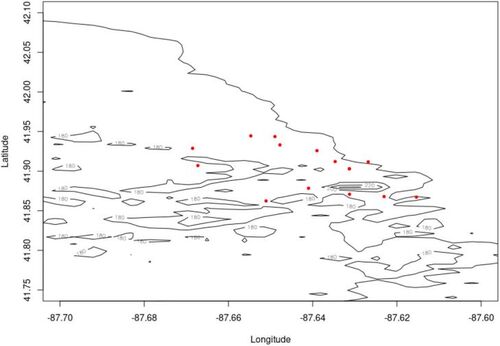Thus, we model the locations as 115 independent draws of a $\text{CMPP}({\Lambda }^{(k)},\nu )$ with quasi-intensity on the k-th day given by (10) $${\Lambda }^{(k)}(s)=\hspace{0.17em}\exp \hspace{0.17em}({\beta }_0+{\beta }_{\text{ele}}x(s)+{\beta }_{\text{temp}}t(k)),$$(10) where x(s) is the elevation at a given location s and t(k) is the air temperature at 11 AM on the k-th day. The Digital Elevation data used is in a 30 m spatial resolution and was obtained from the Alaska Satellite Facility. The temperature covariate was obtained from the National Data Buoy Center, and is the ambient temperature at station CHII2 - Harrison-Dever Crib, Chicago, Illinois. The air temperature is recorded at the station every 10 minutes. It can be freely obtained from https://www.ndbc.noaa.gov/station_history.php?station=chii2. To illustrate the dataset, we are working with, we plot in Figure 4 the locations of the points on 18 May along with a contour plot of the elevation covariate. In implementing the inference method described in Section 2.2, we have used in total 1, 000 dummy points.

Fig. 4 Spatial points on 18 May along with a contour plot of the elevation covariate.

In the null model in which there is no dispersion (ν = 1), the locations are distributed as independent draws of IPP random variables with intensity given by (10)(10) $${\Lambda }^{(k)}(s)=\hspace{0.17em}\exp \hspace{0.17em}({\beta }_0+{\beta }_{\text{ele}}x(s)+{\beta }_{\text{temp}}t(k)),$$(10) . The results for the $\text{CMPP}(\Lambda ,\nu )$ model are reported in Table 5 while the ones for the null Poisson model are shown in Table 6. The 95% bootstrap confidence intervals were computed with 1000 draws from the fitted model. In both models, we find a positive value for ${\beta }_{\text{ele}}$, signalng that a higher elevation is associated with a larger intensity. Indeed, people tend to start their trips at higher elevations and bike downhill. We also observe a positive ${\beta }_{\text{temp}}$, indicating the expected positive association of the intensity of bike rides with temperature. Although the signs of the regression coefficients are comparable between both models, their magnitudes are not (since they model on the one hand a quasi-intensity and on the other an intensity). An analysis following Section 3.3 of the point counts in disjoint regions shows a ubiquitous and statistically significant positive correlation between point counts. For example, if we split the region in two along the y-axis, we estimate a Pearson correlation of point counts of 0.52, with rejection of the null correlation hypothesis with p-value of $2.7·{10}^{-9}$. According to Section 3.3, positive correlation between point counts indicates overdispersion and we thus a priori expect $\nu <1$. This is confirmed by our analysis, and since the bootstrap confidence interval of ν does not contain the value corresponding to the null model ν = 1, in our framework we also reject the null Poisson hypothesis and favor the $\text{CMPP}(\Lambda ,\nu )$ model over the standard Poisson point process. The fitted value of ν is significantly smaller than 1, indicating an overdispersion existing in the highly variable daily Divvy trips that cannot be captured by the standard IPP model. Our model thus jointly models the daily variability in Divvy trips, as well as the spatial locations at which they occur. This enhances the predictive value of our model compared to the IPP which cannot reliably model the overdispersion of daily trips.

Table 5 Estimated parameters in the $\text{CMPP}(\Lambda ,\nu )$ Divvy analysis.

Parameter	Estimated value	Bootstrap confidence interval
β0	–7.79	$(-8.78,-7.03)$
ν	0.30	$(0.017,0.48)$
${\beta }_{\text{temp}}$	0.027	$(0.018,0.042)$
${\beta }_{\text{ele}}$	0.058	$(0.054,0.063)$

Table 6 Estimated parameters in the IPP Divvy analysis.

Parameter	Estimated value	Asymptotic confidence interval
β0	–10.28	$(-11.86,-8.70)$
${\beta }_{\text{temp}}$	0.062	$(0.043,0.081)$
${\beta }_{\text{ele}}$	0.076	$(0.068,0.085)$

In order to properly compare our model to the IPP, we compare the AICs and likelihoods of the logistic regressions corresponding to both models. We report them as “pseudo-AIC” and “pseudo-loglikelihood” in Table 7. Our results confirm that the $\text{CMPP}(\Lambda ,\nu )$ model is favored compared to the model without dispersion, both in terms of AIC and likelihood.

Table 7 Comparison of both models in the Divvy analysis.

Model	Pseudo-AIC	Pseudo-loglikelihood
$\text{CMPP}(\Lambda ,\nu )$	–8365.8	4186.9
IPP	–8285.7	4145.8

4.2 Capeweed

The dataset can be found on the GBIF website, that is, https://www.gbif.org/species/3114986, and consists in the locations of sightings of the species Arctotheca calendula, commonly known as capeweed. The dataset contains each individual’s location, along with the year in which it was spotted. Since the data consists of reports that are not independent samples from the underlying species’ distribution, we rely in our modeling on an observer bias covariate (Fithian et al. 2015) that helps explain why the observed intensity is larger around cities. We use more specifically a bias layer that is a measure of accessibility to cities measured in travel time, and provided by Weiss et al. (2018), see https://malariaatlas.org/research-project/accessibility-to-cities/. 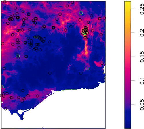Our focus is on yearly sightings between 2012 and 2018, so that our model is seven independent draws of a $\text{CMPP}({\Lambda }^{(k)},\nu )$ with quasi-intensity on the k-th year given by (11) $${\Lambda }^{(k)}(s)=\hspace{0.17em}\exp \hspace{0.17em}\left[{\beta }_0+\sum _{i=1}^p{\beta }_i{X}_i^{(k)}(x)+\gamma Y(x)\right],$$(11) where $X_1^{(k)},\dots ,X_p^{(k)}$ are environmental covariates thought to be important in explaining the distribution of the species, and Y(x) is the accessibility to city bias layer from Weiss et al. (2018). Regarding the environmental covariates, we choose as a purely spatial covariate the pH of the soil at a given location, which can be found at https://www.clw.csiro.au/aclep/soilandlandscapegrid. We also choose as a spatiotemporal covariate the maximum temperature in October of the corresponding year, available from WorldClim at https://worldclim.org/data/monthlywth.html. To illustrate the dataset we are working with, we plot in Figure 5 the locations of all data points considered, as well as the predicted quasi-intensity in 2018. We have used in total 10, 000 dummy points when implementing the method described in Section 2.2.

Fig. 5 Sightings of capeweed between 2012 and 2018 in South-East Australia (in black) with those in year 2017 highlighted in green, along with the predicted quasi-intensity in 2017.

The results for the $\text{CMPP}(\Lambda ,\nu )$ model are reported in Table 8 while the ones for the null Poisson model (ν = 1) are shown in Table 9. As in the previous case study, the 95% bootstrap confidence intervals were computed with 1000 draws from the fitted model.

Table 8 Estimated parameters in the $\text{CMPP}(\Lambda ,\nu )$ capeweed analysis.

Parameter	Estimated value	Bootstrap confidence interval
β0	–10.28	$(-11.68,-8.95)$
ν	0.15	$(0.075,0.27)$
${\beta }_{\text{pH}}$	0.79	$(0.38,1.13)$
${\beta }_{{\mathrm{t}}_{\max }}$	0.24	$(0.17,0.32)$
γ	–0.011	$(-0.013,-0.0090)$

Table 9 Estimated parameters in the IPP capeweed analysis.

Parameter	Estimated value	Asymptotic confidence interval
β0	–7.84	$(-10.83,-4.85)$
${\beta }_{\text{pH}}$	0.72	$(0.019,1.43)$
${\beta }_{{\mathrm{t}}_{\max }}$	0.28	$(0.14,0.41)$
γ	–0.011	$(-0.016,-0.0066)$

The bias layer is found to be an important covariate. The negative value of its corresponding estimated coefficient confirms that locations close to cities have a higher intensity of reported capeweed individuals. The other two environmental covariates, namely soil pH and the maximum temperature in October, are also found to be important drivers of the distribution of capeweed. Finally, and perhaps more importantly, ν is found to be close to zero, signifying overdispersion from year to year in the number of capeweed reports. Quantifying the overdispersion helps ecologists better understand how volatile the total number of capeweed individuals is from year to year. In addition, since the bootstrap confidence interval of ν does not contain the value corresponding to the null model ν = 1, we reject the null IPP hypothesis and favor the $\text{CMPP}(\Lambda ,\nu )$ model. More precisely, we compare the AICs and likelihoods of the logistic regressions corresponding to both models. We report them as “pseudo-AIC” and “pseudo-loglikelihood” in Table 10. In this study too, our findings confirm that the $\text{CMPP}(\Lambda ,\nu )$ model is favored compared to the model without dispersion, both in terms of AIC and likelihood.

Table 10 Comparison of both models in the capeweed analysis.

Model	Pseudo-AIC	Pseudo-loglikelihood
$\text{CMPP}(\Lambda ,\nu )$	–631.3	320.6
IPP	–587.6	297.8

4.3 Flooding of the Rio Negro river

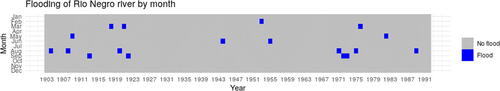
In this subsection, we consider monthly records of the flooding of the Rio Negro river in Manaus, Brazil between 1903 and 1992. A yearly version of this data was studied in Example 2 in Zhu et al. (2017), see also Brillinger (1995) for the original study. In order to recover the month in which a flooding occurred, we used the R dataset boot::manaus which contains the river heights on the focal period. We analyze the data as a homogeneous point process on the temporal window $W=[1903,1992]$, see Figure 6. This analysis differs from that of the previous two studies in some important ways. First, the data are analyzed as a temporal point process, with events being times rather than locations. Second, it has been found to be underdispersed, meaning that there is some regularity in flooding occurrences.

Fig. 6 Monthly records of the flooding of the Rio Negro river in Manaus, Brazil between 1903 and 1992.

The results for the $\text{CMPP}(\Lambda ,\nu )$ model are reported in Table 11. The 95% bootstrap confidence intervals were computed with 10, 000 draws from the fitted model, and we have used in total 10, 000 dummy points. The analysis was also conducted under the null Poisson model (ν = 1), with results reported in Table 12.

Table 11 Estimated parameters in the $\text{CMPP}(\Lambda ,\nu )$ Rio Negro river analysis.

Parameter	Estimated value	Bootstrap confidence interval
β0	–1.386	$(-1.972,-0.901)$
ν	24.04	$(23.19,24.74)$

Table 12 Estimated intercept parameter in the IPP Rio Negro river analysis.

Parameter	Estimated value	Asymptotic confidence interval
β0	–1.609	$(-2.261,-0.957)$

Similarly to the findings of Zhu et al. (2017), we find that the data are significantly underdispersed. However, as discussed in the introduction and proved in Proposition 1, their model is not well defined in the non Poissonian case. Therefore, we believe our analysis of this dataset, although done in the same time-homogeneous framework of Zhu et al. (2017), is more theoretically sound than that of Zhu et al. (2017). The confidence interval for the estimation of the dispersion parameter ν unambiguously excludes the null hypothesis corresponding to the IPP case ν = 1. We also compare the AICs and likelihoods of the logistic regressions corresponding to both models, and we report them as “pseudo-AIC” and “pseudo-loglikelihood” in Table 13. Our results in Table 13 confirm that the $\text{CMPP}(\Lambda ,\nu )$ model is favored compared to the model without dispersion, both in terms of AIC and likelihood.

Table 13 Comparison of both models in the Rio Negro river analysis.

Model	Pseudo-AIC	Pseudo-loglikelihood
$\text{CMPP}(\Lambda ,\nu )$	–72.1	38.0
IPP	–66.1	34.0

5 Discussion

In this article, we have introduced the $\text{CMPP}(\Lambda ,\nu )$ as a class of spatial point processes that is more flexible than the inhomogeneous Poisson process model. This allows us to tackle spacial point patterns with a range of variance-to-mean ratios. When there is a single spatial point pattern, it seems impossible to estimate the variance-to-mean ratio so a common approach is to use the IPP, in effect imposing ν = 1. If there are replicated point patterns, it becomes crucial to consider correlations between different regions. Figure 2 shows that the $\text{CMPP}(\Lambda ,\nu )$ captures positive and negative correlations between point counts in different locations, which the IPP fails to do, see Figure 3. We have derived a formula for the point count correlation in Proposition 2 making explicit the relation between point count correlation and the dispersion parameter ν.

The logistic regression (Baddeley et al. 2014) has been employed to fit our proposed $\text{CMPP}(\Lambda ,\nu )$ process, and its usefulness has been demonstrated through numerical simulations. Our model is analytically tractable and we have made explicit some of its theoretical properties. In particular, we are able to compute the Janossy density of its restriction to a subregion (Proposition 3) and its intensity function can be computed explicitly (Proposition 4). The case studies further show that the proposed model has outperformed the Poisson model in a variety of applications involving replicated point patterns.

We remark that in the case of independent and identical samples, the quasi-intensity of the $\text{CMPP}(\Lambda ,\nu )$ is proportional to that of the Poisson point process. As such, a quasi-intensity that depends log-linearly on covariates via (2)(2) $$\hspace{0.17em}\ln \hspace{0.17em}(\Lambda (s))={\beta }_0+\sum _{j=1}^m{\beta }_j{x}_j(s),$$(2) will have the same parameter estimates of ${\beta }_1,\dots ,{\beta }_m$ as the corresponding Poisson point process. The intercept β₀ and the dispersion parameter ν can then be found by analyzing the maximum likelihood estimator corresponding to point counts.

Our work illustrates some of the difficulties involved when working with replicated point patterns, and the complex theoretical ideas that need to be taken into account whenever there is spatial correlation in datasets. Since replicated point patterns are frequently encountered in practice, the avenue of research initiated here should be considered an important first step paving the way for future work in this area. One area that might be of particular interest is the model’s inclusion of a time-varying ν, generalizing the work in Wu, Holan, and Wikle (2013) to the point process setting. This is complicated by the fact that in our framework ν affects both the dispersion of average total point counts, as well as the intensity indirectly through Proposition 4. The time-varying model on ν should thus be carefully parametrized so as to separate both effects. One could also consider generalizations of the CMP distribution such as that introduced in Imoto (2014) and Qian and Zhu (2023).

Data availability

The data used in our case studies is available online. The Divvy dataset can be obtained from https://data.cityofchicago.org. The capeweed data can be found on the GBIF website, i.e., https://www.gbif.org/species/3114986. The Rio Negro river flooding can be imported through the R dataset boot::manaus.

Additional information

Funding

Research supported by ARC Discovery Grant DP150101459 (AX), ARC Discovery Grant DP150102472 (YW) and ARC Grant DP190100613 (IF, AX and YW).

Appendix

Proposition 1.

Let Ξ be a point process on $[0,T]$ with T > 0 such that $\Xi ([0,T])$ follows a CMP distribution (1)(1) $$f(i)=\frac{{\lambda }^i}{Z(\lambda ,\nu ){(i!)}^{\nu }},\hspace{1em}i\in {\mathbb{Z}}_{+}:=\{0,1,2,\dots \},$$(1) with $\nu >0$. If Ξ has independent and stationary increments, then Ξ is a time homogeneous Poisson process.

Proof.

For each positive integer n, we divide $[0,T]$ into n subintervals $A_0:=[0,T/n],A_i:=(iT/n,(i+1)T/n],1\le i\le n-1$. Then the numbers of points $\Xi (A_i),0\le i\le n-1$, are iid random variables, hence the distribution of $\Xi ([0,T])$ is infinitely divisible. Since $\Xi ([0,T])$ follows a CMP distribution with $\nu >0$, Geng and Xia (2022) used the entire function to show that an infinitely divisible CMP distribution with $\nu >0$ must satisfy ν = 1, we conclude that $\Xi ([0,T])$ is a Poisson random variable. Therefore, it follows from Raikov’s theorem (see Section 19.2 of Loève 1963) that $\Xi (A_i),0\le i\le n-1$, for all $n\ge 1$, are Poisson random variables. This implies that Ξ is a time homogeneous Poisson process. □

Proposition 2.

Let W₁, W₂ be a partition of W and let Y₁ and Y₂ denote the counts of points in regions W₁ and W₂, and p₁ and p₂ be the probabilities of points falling into W₁ and W₂, respectively. Then the correlation coefficient between Y₁ and Y₂ satisfies (A.1) $$\text{Corr}(Y_1,Y_2)=\frac{\sqrt{p_1{p}_2}(\text{Var}(N)-\mathbb{E}N)}{\sqrt{(p_2\mathbb{E}N+p_1\text{Var}(N))(p_1\mathbb{E}N+p_2\text{Var}(N))}}.$$(A.1)

Proof.

Conditional on N, Y_i is a binomial B $(N,p_i)$ so $$\begin{array}{c}\mathbb{E}{Y}_i=\mathbb{E}[\mathbb{E}(Y_i|N)]=\mathbb{E}[p_{i}N]=p_i\mathbb{E}N;\\ \text{Var}(Y_i)=\mathbb{E}\text{Var}(Y_i|N)+\text{Var}(\mathbb{E}(Y_i|N))\\ =\mathbb{E}[N{p}_i(1-p_i)]+\text{Var}(p_{i}N)=p_i(1-p_i)\mathbb{E}N+p_i^2\text{Var}(N);\\ \text{Cov}(Y_1,Y_2)=\frac{1}{2}[\text{Var}(N)-\text{Var}(Y_1)-\text{Var}(Y_2)]=p_1{p}_2(\text{Var}(N)-\mathbb{E}N).\end{array}$$

The stated result (A.1)(A.1) $$\text{Corr}(Y_1,Y_2)=\frac{\sqrt{p_1{p}_2}(\text{Var}(N)-\mathbb{E}N)}{\sqrt{(p_2\mathbb{E}N+p_1\text{Var}(N))(p_1\mathbb{E}N+p_2\text{Var}(N))}}.$$(A.1) is an immediate consequence of these equalities. □

Depending on the dispersion parameter ν, the CMP distribution can be used to model both underdispersion and overdispersion distributions (Conway and Maxwell 1962). Specifically when $\nu <1,\text{Var}(N)>\mathbb{E}N$ and $\text{Var}<\mathbb{E}N$ when $\nu >1$. Therefore the correlation coefficient given in (A.1)(A.1) $$\text{Corr}(Y_1,Y_2)=\frac{\sqrt{p_1{p}_2}(\text{Var}(N)-\mathbb{E}N)}{\sqrt{(p_2\mathbb{E}N+p_1\text{Var}(N))(p_1\mathbb{E}N+p_2\text{Var}(N))}}.$$(A.1) is either positive or negative depending on ν. When ν = 1, that is, in the case of the Poisson distribution, the correlation coefficient $\text{Corr}(Y_1,Y_2)$ becomes zero.

Proposition 3.

The Janossy density of a $\text{CMPP}(\Lambda ,\nu )$ restricted to $D\subset W$ is $$j_D(\{x_1,\dots ,x_n\})=\frac{\prod _{i=1}^n\Lambda (x_i)}{Z(\mathcal{l}(\Lambda ),\nu )}\sum _{m=n}^{\infty }\frac{\Lambda {(W\backslash D)}^{m-n}}{(m-n)!{(m!)}^{\nu -1}},\hspace{1em}\{x_1,\dots ,x_n\}\subset D,$$where $\Lambda (W\backslash D):={\int }_{W\backslash D}\Lambda (x) \mathrm{d}x.$

Proof.

We use (3)(3) $$j(\{x_1,\dots ,x_n\})=\frac{1}{Z(\mathcal{l}(\Lambda ),\nu ){(n!)}^{\nu -1}}\prod _{i=1}^n\Lambda (x_i),\hspace{1em}\{x_1,\dots ,x_n\}\subset W.$$(3) and integrate over all points outside D to get $$\begin{array}{c}{j}_D(\{x_1,\dots ,x_n\})=\sum _{m=n}^{\infty }\frac{\prod _{i=1}^n\Lambda (x_i)}{Z(\mathcal{l}(\Lambda ),\nu ){(m!)}^{\nu -1}}{\int }_{W\backslash D}\dots {\int }_{W\backslash D}\prod _{j=n+1}^m(\Lambda (x_j) \mathrm{d}{x}_j)\\ =\frac{\prod _{i=1}^n\Lambda (x_i)}{Z(\mathcal{l}(\Lambda ),\nu )}\sum _{m=n}^{\infty }\frac{\Lambda {(W\backslash D)}^{m-n}}{(m-n)!{(m!)}^{\nu -1}},\end{array}$$as claimed. □

Proposition 4.

The intensity of a $\text{CMPP}(\Lambda ,\nu )$ is given by $$\varrho (x)=\frac{\Lambda (x)\mathbb{E}\left[N\right]}{\mathcal{l}(\Lambda )},x\in W.$$

Proof.

Let g be a non negative measurable function defined on W. Denoting by Ξ a $\text{CMPP}(\Lambda ,\nu )$ point process and by ${(X_i)}_{i\ge 1}$a sequence of iid random variables with distribution $\Lambda /\mathcal{l}(\Lambda )$, we have $$\begin{array}{c}\mathbb{E}\left[\sum _{x\in \Xi }g(x)\right]=\sum _{n\ge 0}\mathbb{E}\left[\sum _{i=1}^{n}g(X_i)\right]\mathbb{P}(N=n)\\ =\sum _{n\ge 0}\mathbb{E}[g(X_1)]n\mathbb{P}(N=n)\\ =\mathbb{E}[g(X_1)]\mathbb{E}\left[N\right]\\ =\frac{{\int }_{W}g(x)\Lambda (x) \mathrm{d}x}{\mathcal{l}(\Lambda )}\mathbb{E}\left[N\right]\\ ={\int }_{W}g(x)\frac{\Lambda (x)\mathbb{E}\left[N\right]}{\mathcal{l}(\Lambda )} \mathrm{d}x.\end{array}$$

Since g can in particular be chosen in the class of indicator functions of subsets of W, the claim follows. □

References

- Alqawba, M., and N. Diawara. 2021. Copula-based Markov zero-inflated count time series models with application. Journal of Applied Statistics 48 (5):786–803. doi: 10.1080/02664763.2020.1748581.35707445.
- Andrews, J., R. Ganti, M. Haenggi, N. Jindal, and S. Weber. A primer on spatial modeling and analysis in wireless networks. IEEE Communications Magazine 48 (11):156–63. doi: 10.1109/MCOM.2010.5621983.
- Babu, G. J., and E. D. Feigelson. 1996. Spatial point processes in astronomy. Journal of Statistical Planning and Inference 50 (3):311–26. doi: 10.1016/0378-3758(95)00060-7.
- Baddeley, A., J.-F. Coeurjolly, E. Rubak, and R. Waagepetersen. 2014. Logistic regression for spatial Gibbs point processes. Biometrika 101 (2):377–92. doi: 10.1093/biomet/ast060.
- Baddeley, A., E. Rubak, and R. Turner. 2015. Spatial point patterns: Methodology and applications. London: Chapman and Hall/CRC Press.
- Baddeley, A., and R. Turner. 2000. Practical maximum pseudolikelihood for spatial point patterns. Australian & New Zealand Journal of Statistics 42 (3):283–322. doi: 10.1111/1467-842X.00128.
- Brillinger, D. R. 1995. Trend analysis: binary-valued and point cases. Stochastic Hydrology and Hydraulics 9 (3):207–13. doi: 10.1007/BF01581719.
- Coeurjolly, J.-F., and E. Rubak. 2013. Fast covariance estimation for innovations computed from a spatial Gibbs point process. Scandinavian Journal of Statistics 40 (4):669–84. doi: 10.1111/sjos.12017.
- Connor, C. B., and B. E. Hill. 1995. Three nonhomogeneous Poisson models for the probability of basaltic volcanism: Application to the Yucca Mountain region, Nevada. Journal of Geophysical Research: Solid Earth 100 (B6):10107–25. doi: 10.1029/95JB01055.
- Conway, R. W., and W. L. Maxwell. 1962. A queuing model with state dependent service rates. Journal of Industrial Engineering 12:132–6.
- Daley, D. J., and D. Vere-Jones. 2003. An introduction to the theory of point processes: Volume I: Elementary theory and method. New York: Springer-Verlag.
- Daley, D. J., and D. Vere-Jones, 2008. An introduction to the theory of point processes. In Probability and its applications. Vol. 2. New York: Springer-Verlag.
- Diggle, P. J., and R. K. Milne. 1983. Negative binomial quadrat counts and point processes. Scandinavian Journal of Statistics 10:257–67.
- Fithian, W., J. Elith, T. Hastie, and D. A. Keith. 2015. Bias correction in species distribution models: Pooling survey and collection data for multiple species. Methods in Ecology and Evolution 6 (4):424–38. doi: 10.1111/2041-210X.12242.27840673.
- Geng, X., and A. Xia. 2022. When is the conway-maxwell-poisson distribution infinitely divisible?. Statistics & Probability Letters 181:109264. doi: 10.1016/j.spl.2021.109264.
- Huang, A. 2017. Mean-parametrized Conway–Maxwell–Poisson regression models for dispersed counts. Statistical Modelling 17 (6):359–80. doi: 10.1177/1471082X17697749.
- Imoto, T. 2014. A generalized Conway–Maxwell–Poisson distribution which includes the negative binomial distribution. Applied Mathematics and Computation 247:824–34. doi: 10.1016/j.amc.2014.09.052.
- Kroese, D. P., and Z. I. Botev, 2015. Spatial process simulation. In Stochastic geometry, Spatial statistics and random fields, 369–404. Cham: Springer.
- Li, X., and D. K. Dey. 2022. Estimation of COVID-19 mortality in the United States using Spatio-temporal Conway Maxwell Poisson model. Spatial Statistics 49:377–92. doi: 10.1016/j.spasta.2021.100542.
- Loève, M. 1963. Probability theory, 3rd ed. New York: Van Nostrand.
- MacDonald, I. L., and F. Bhamani. 2020. A time-series model for underdispersed or overdispersed counts. The American Statistician 74 (4):317–28. doi: 10.1080/00031305.2018.1505656.
- Mannering, F. L, and C. R. Bhat. 2014. Analytic methods in accident research: Methodological frontier and future directions. Analytic Methods in Accident Research 1:1–22. doi: 10.1016/j.amar.2013.09.001.
- Melo, M., and A. Alencar. 2020. Conway–Maxwell–Poisson autoregressive moving average model for equidispersed, underdispersed, and overdispersed count data. Journal of Time Series Analysis 41 (6):830–57. doi: 10.1111/jtsa.12550.
- Minka, T. P., G. Shmeuli, J. B. Kadane, S. Borle, and P. Boatwright. 2002. Computing with the com-poisson distribution. Technical Report 776. Department of Statistics, Carnegie Mellon University, Pittsburgh, PA.
- Qian, L., and F. Zhu. 2023. A flexible model for time series of counts with overdispersion or underdispersion, zero-inflation and heavy-tailedness. Communications in Mathematics and Statistics
- Ribeiro, E. E., W. M. Zeviani, W. H. Bonat, C. G. Demetrio, and J. Hinde. 2020. Reparametrization of COM–Poisson regression models with applications in the analysis of experimental data. Statistical Modelling 20 (5):443–66. doi: 10.1177/1471082X19838651.
- Sellers, K. F., S. Borle, and G. Shmueli. 2012. The COM-Poisson model for count data: a survey of methods and applications. Applied Stochastic Models in Business and Industry 28 (2):104–16. doi: 10.1002/asmb.918.
- Sellers, K. F, and G. Shmueli. 2010. A flexible regression model for count data. Annals of Applied Statistics 4:943–61.
- Thompson, H. R. 1955. Spatial point processes, with applications to ecology. Biometrika 42 (1-2):102–15. doi: 10.1093/biomet/42.1-2.102.
- Waller, L. A., and C. A. Gotway. 2004. Applied spatial statistics for public health data, Vol. 368. New Jersey: John Wiley and Sons.
- Weiss, C., F. Zhu, and A. Hoshiyar. 2020. Softplus ingarch models. Statistica Sinica 32:1099–120. doi: 10.5705/ss.202020.0353.
- Weiss, D. J., A. Nelson, H. S. Gibson, W. Temperley, S. Peedell, A. Lieber, M. Hancher, E. Poyart, S. Belchior, N. Fullman, et al. 2018. A global map of travel time to cities to assess inequalities in accessibility in 2015. Nature 553 (7688):333–6. 29320477 doi: 10.1038/nature25181.
- Wu, G., S. H. Holan, and C. K. Wikle. 2013. Hierarchical Bayesian spatio-temporal Conway–Maxwell Poisson models with dynamic dispersion. Journal of Agricultural, Biological, and Environmental Statistics 18 (3):335–56. doi: 10.1007/s13253-013-0141-2.
- Zhu, F. 2012. Modeling time series of counts with COM-Poisson INGARCH models. Mathematical and Computer Modelling 56 (9-10):191–203. doi: 10.1016/j.mcm.2011.11.069.
- Zhu, L., K. F. Sellers, D. S. Morris, and G. Shmueli. 2017. Bridging the gap: A generalized stochastic process for count data. The American Statistician 71 (1):71–80. doi: 10.1080/00031305.2016.1234976.