Bayesian inference using least median of squares and least trimmed squares in models with independent or correlated errors and outliers

Abstract

We provide Bayesian inference in the context of Least Median of Squares and Least Trimmed Squares, two well-known techniques that are highly robust to outliers. We apply the new Bayesian techniques to linear models whose errors are independent or AR and ARMA. Model comparison is performed using posterior model probabilities, and the new techniques are examined using Monte Carlo experiments as well as an application to four portfolios of asset returns.

KEYWORDS:

• Bayesian inference
• least Median of squares
• least trimmed squares
• stochastic volatility
• ARMA models
• outliers

1 Introduction

In an important paper, Piradl, Shadrokh, and Yarmohammadi (PSY 2021) propose to use a robust estimation method with autocorrelated errors. PSY use the minimum Matusita distance estimation method and introduce a new robust estimation method for the linear regression model with correlated error terms in the presence of outliers, and compare it with M-estimation and the well-known Cochrane and Orcutt least squares estimation method (Matusita 1953, 1955, 1964). In this article, we propose an alternative approach based on Bayesian implementation of Least Median of Squares and Least Trimmed Squares (Rousseeuw 1984) for independent errors as well as autocorrelated errors. In Section 2, we present the Least Median of Squares and Least Trimmed Squares procedures with uncorrelated errors. In Section 3, we extend to correlated errors of the AR and ARMA variety where we also present Monte Carlo evidence. In Section 4 we present an empirical application and we provide model comparison.

2 Least median of squares with uncorrelated errors

Rousseeuw (1984) proposed the method of Least Median of Squares (LMS) in which the sum of squared residuals used in Least Squares (LS) is replaced by the median of the squared residuals. The resulting estimator can resist the effect of nearly 50% of contamination in the data. As he argued convincingly: “Let us now return to [least squares method]”. A more complete name for the LS method would be least sum of squares, but apparently few people have objected to the deletion of the word “sum-as if the only sensible thing to do with n positive numbers would be to add them” (Rousseeuw 1984, p. 872). Given a regression model: (1) $$y_t=x_t^{\prime }\beta +u_t,t=1,\dots ,n,$$(1) where x_t is a $k\times 1$ vector of explanatory variables, β is a $k\times 1$ parameter vector of and u_t represents an error term, LMS produces the estimator: (2) $$\widehat{\beta }=\arg \underset{{}_{\beta }}{\min }\underset{t=1,\dots ,n}{\mathit{median}}{(y_t-x_t^{\prime }\beta )}^2,$$(2) where “med” denotes the median. Rousseeuw (1984) intended his method as an exploratory data analysis tool and did not work on standard errors for the coefficients β. Moreover, computational problems associated with LMS are still open to this day.

Bayesian analysis of LMS has not been attempted due to its computational difficulties but also the fact that there is no obvious way to connect it to a likelihood function. For example, LS is associated with the normal distribution, the Least Absolute Deviations (LAD) estimator is associated with the Laplace distribution, etc. However, in the case of LMS, it is not obvious how to proceed in terms of Bayesian analysis.

Bissiri, Holmes, and Walker (2016) have shown how to update beliefs in a Bayesian framework when we do not have a likelihood function but we do have a loss function.¹ Given a parameter $\theta \in \Theta \subseteq {\mathfrak{R}}^d$, and data Y, they show that given a prior $p(\theta )$ the update to a posterior $p(\theta |Y)$, can be made using: (3) $$p(\theta |Y)\propto p(\theta )\hspace{0.17em}\exp \hspace{0.17em}\left\{-\mathcal{l}(\theta ,Y)\right\},$$(3) where $\mathcal{l}(\theta ,Y)\ge 0$ is a certain loss function. For estimating a median, one would take $\mathcal{l}(\theta ,Y)=|\theta -Y|$ while for estimating a mean, $\mathcal{l}(\theta ,Y)={(\theta -Y)}^2$ when it so happens that Y is a single observation. Of course, expected loss is: $L(\theta )=\int \mathcal{l}(\theta ,Y)\mathrm{d}F(Y)$ where F(Y) is a distribution function associated with the data.

Given (3)(3) $$p(\theta |Y)\propto p(\theta )\hspace{0.17em}\exp \hspace{0.17em}\left\{-\mathcal{l}(\theta ,Y)\right\},$$(3) , we can further extend the update by using the posterior: (4) $$p(\theta ,h|Y)\propto p(\theta )h^{n-1}\hspace{0.17em}\exp \hspace{0.17em}\left\{-h\mathcal{l}(\theta ,Y)\right\},$$(4) where h is a scale parameter whose prior is: $p(h)\propto h^{-1}$. Using well-known properties of the gamma distribution, we have: (5) $$\begin{array}{ccc}p(\theta |Y)& =& {\int }_0^{\infty }p(\theta ,h|Y)\propto p(\theta ){\int }_0^{\infty }{h}^{n-1}\hspace{0.17em}\exp \hspace{0.17em}\left\{-h\mathcal{l}(\theta ,Y)\right\}\\ & =& p(\theta ){\left\{\mathcal{l}(\theta ,Y)\right\}}^{-n/2}.\end{array}$$(5)

If the prior is flat (viz. $p(\theta )\propto \text{const}.,\theta \in \Theta$) or at least we can reasonably assume that it is bounded above, integrability of (5)(5) $$\begin{array}{ccc}p(\theta |Y)& =& {\int }_0^{\infty }p(\theta ,h|Y)\propto p(\theta ){\int }_0^{\infty }{h}^{n-1}\hspace{0.17em}\exp \hspace{0.17em}\left\{-h\mathcal{l}(\theta ,Y)\right\}\\ & =& p(\theta ){\left\{\mathcal{l}(\theta ,Y)\right\}}^{-n/2}.\end{array}$$(5) may be a problem. The problem can be always avoided if we assume that the scale parameter has the following prior: (6) $$p(h|\beta )\propto h^{-1}\hspace{0.17em}\exp \hspace{0.17em}\left\{-\underset{¯}{q}h\right\},$$(6) where $\underset{¯}{q}>0$. This is still an improper prior but the posterior is proper as, after integrating h out, we have: (7) $$p(\theta |Y)\propto p(\theta ){\left\{\underset{¯}{q}+\mathcal{l}(\theta ,Y)\right\}}^{-n/2}.$$(7)

Given the stated conditions on the prior of θ, the only assumption we needed for integrability of the posterior is: $\mathcal{l}(\theta ,Y)\ge 0>\forall \theta \in \Theta$. Clearly, the “non informative” choice would be to select $\underset{¯}{q}$ as close to zero as possible (we use ${10}^{-7}$ in this study).

In turn, given the posterior kernel in (5)(5) $$\begin{array}{ccc}p(\theta |Y)& =& {\int }_0^{\infty }p(\theta ,h|Y)\propto p(\theta ){\int }_0^{\infty }{h}^{n-1}\hspace{0.17em}\exp \hspace{0.17em}\left\{-h\mathcal{l}(\theta ,Y)\right\}\\ & =& p(\theta ){\left\{\mathcal{l}(\theta ,Y)\right\}}^{-n/2}.\end{array}$$(5) standard Bayesian Markov Chain Monte Carlo (MCMC) methods (Hastings 1970; Tierney 1994) can be used to provide samples $\left\{{\theta }^{(s)},s=1,\dots ,S\right\}$ that converge to the distribution whose kernel density is given by (5)(5) $$\begin{array}{ccc}p(\theta |Y)& =& {\int }_0^{\infty }p(\theta ,h|Y)\propto p(\theta ){\int }_0^{\infty }{h}^{n-1}\hspace{0.17em}\exp \hspace{0.17em}\left\{-h\mathcal{l}(\theta ,Y)\right\}\\ & =& p(\theta ){\left\{\mathcal{l}(\theta ,Y)\right\}}^{-n/2}.\end{array}$$(5) .

In the case of LMS regression, where it is natural to assume that the distribution of the errors involves a scale parameter h, the posterior becomes: (8) $$p(\beta |Y)\propto p(\beta ){\left\{\underset{¯}{q}+\underset{t=1,\dots ,n}{\mathit{median}}{(y_t-x_t^{\prime }\beta )}^2\right\}}^{-n/2}.$$(8)

A related idea is to use least trimmed squares (LTS, see also Rousseeuw 1984). This estimator has the following loss function: (9) $$l(\beta ,Y)=\sum _{t=1}^H{(r_t)}_{1:H}^2,$$(9) where ${(r_t)}_{1:H}^2$ are the ordered squared residuals. Generally, H depends on the trimming proportion α, so that: $H=1+\left[n(1-\alpha )\right]$, where $[·]$ denotes the integer part.

3 Least median of squares with correlated errors

We consider (1)(1) $$y_t=x_t^{\prime }\beta +u_t,t=1,\dots ,n,$$(1) under the assumption (10) $$u_t=\rho u_{t-1}+e_t,$$(10) where $e_t\sim \mathrm{i}.\mathrm{i}.\mathrm{d}\mathcal{N}(0,{\sigma }^2)$. Therefore, we have (11) $$y_t=\rho y_{t-1}+{(x_t-\rho x_{t-1})}^{\prime }\beta +e_t.$$(11)

Therefore, the LMS posterior (8)(8) $$p(\beta |Y)\propto p(\beta ){\left\{\underset{¯}{q}+\underset{t=1,\dots ,n}{\mathit{median}}{(y_t-x_t^{\prime }\beta )}^2\right\}}^{-n/2}.$$(8) becomes (12) $$p(\beta |Y)\propto p(\beta )\left\{\underset{¯}{q}+\underset{t=1,\dots ,n}{\mathit{median}}{(y_t-\rho y_{t-1}-{(x_t-\rho x_{t-1})}^{\prime }\beta )}^2\right\}{.}^{-n/2}$$(12)

For LTS the posterior becomes (13) $$p(\beta |Y)\propto p(\beta )\left\{\underset{¯}{q}+{\left[{(y_t-\rho y_{t-1}-{(x_t-\rho x_{t-1})}^{\prime }\beta )}^2\right]}_{1:H}\right\}{.}^{-n/2}$$(13)

3.1 Results with independent data

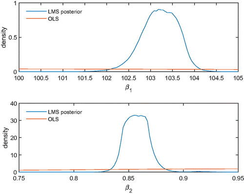
Next, we present a numerical example to see how LMS and LTS perform in relation to least squares. Raj and Senthamarai (2017) use a regression to examine the relationship between blood pressure and age in 30 patients. In Figure 1, we present the marginal posteriors of the intercept (upper panel) and the slope (lower panel) compared to a normal distribution for OLS parameter estimates. This is really a sampling distribution; viz., a normal distribution, over the appropriate range defined by LMS/LTS, centered at the OLS estimate, and having variance the familiar OLS expression. As a result of contamination, the sampling distribution of OLS has a large variance and appears as flat over the posterior domain of LMS/LTS. Clearly, LMS performs excellently, whereas the sampling distribution of OLS has no posterior probability over the domain of LMS.²

Fig. 1 Bayesian LMS of blood pressure data.

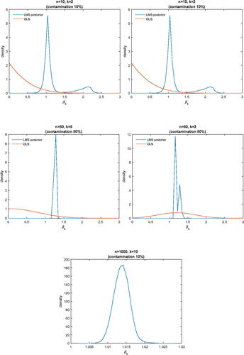
In Figure 2, we report marginal posterior densities of β_k in a regression model with n observations and k regressors. In the regression, there is always an intercept, and k – 1 normally distributed regressors (i.i.d). The regression coefficients are all set equal to 1. With degree of contamination c, the errors are generated from a standard normal distribution with probability $1-c$, and a standard Cauchy (Student-t with one degree of freedom) with probability c. Again, the sampling distribution of OLS places, practically, no posterior probability around the true values (which are all equal to 1).

Fig. 2 Marginal posterior densities with different n, k, and degree of contamination.

3.2 Monte Carlo experiment for correlated errors

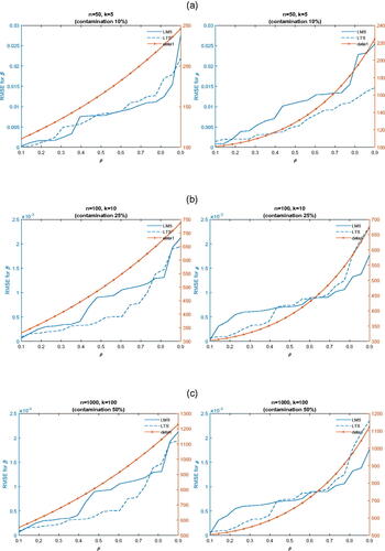
We keep the same configurations as in the previous subsection, but we now assume that errors are autocorrelated as in (10)(10) $$u_t=\rho u_{t-1}+e_t,$$(10) . We vary the autocorrelation coefficient from $\rho =0.1$ to 0.9 (20 different values). Our Monte Carlo experiment uses 1,000 replications, 15,000 MCMC draws, omitting the first 5,000 in the burn-in phase. We are interested in the median bias of OLS, LMS, and LTS estimates of parameter vector β (across all its components whose true values are all equal to 1) for different configurations of n, k, ρ, and degree of contamination. The initial value for errors (u₀) is taken to be zero in all cases. We present our Monte Carlo results in graphical form to facilitate reading. In Figure 3, we report root mean squared errors of parameters β (left panel) and ρ (right panel) for LMS and LTS posteriors as well as the normal posterior of OLS that takes into account the AR(1) model in (10)(10) $$u_t=\rho u_{t-1}+e_t,$$(10) . In panel (a), we report results for a small sample and a few regressors with contamination 10%. In panel (b), we report results for a medium sample and a moderate number regressors with contamination 25%. Finally, in panel (c) we report results for a large sample and a large number regressors with contamination 50%. LMS and LTS posteriors deliver results that are esstinally unbiased in samples whose size is as small as 50, whereas standard AR(1) estimation delivers estimators whose bias is orders of magnitude larger compared to LMS or LTS. ³

Fig. 3 RMSE of parameters (β) and ρ.

4 Empirical application

4.1 Statistical inference

It is well known that volatility in asset markets is autocorrelated, a fact that is known as “volatility clustering”. Techniques that are used in the literature include Generalized Autoregressive Conditional Heteroskedasticity (GARCH) or Stochastic Volatility (SV) models. If r_t denotes the return of a certain asset, we define volatility as $y_t=\hspace{0.17em}\log \hspace{0.17em}{r}_t^2$ as the mean return is, practically, zero. However, it is also well known that asset returns are often leptokurtic; therefore, we expect a certain number of outliers or contamination that may affect adversely estimates of μ and ρ.

We use four value-weighted equity portfolios formed by sorting individual stocks based on market capitalization of equity (ME) and book-to-market equity ratio (BM). The sample period is from January 1963 to December 2020. Monthly percentage returns in excess of the T-bill rate are analyzed in the first two applications; the third application uses daily excess returns. The data are from Kenneth French’s data library, which uses security level data from the CRSP, Compustat, and Ibbotson Associates data bases.

In turn, we use the following model $$\begin{array}{c}{y}_t=\mu +u_t,\\ u_t=\rho u_{t-1}+e_t.\end{array}$$

We are especially interested in estimates of ρ to determine the degree of persistence in volatility. The results are reported in Figure 4. Clearly, in all cases, the AR(1) posterior mean. This indicates that there are indeed outliers which affect the posterior of AR(1)⁴ is shifted to the right relative to the LMS and LTS posteriors (which are nearly the same).

Fig. 4 Marginal posterior densities of ρ.

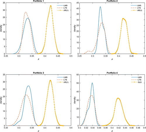
Clearly, the marginal posteriors of ρ are nearly the same for LMS and LTS but quite different compared to the marginal posterior of ρ from AR(1) estimation. In turn, this indicates that the presence of outliers in volatility affects AR(1) estimation in a significant way.

4.2 More general models

The extension of the new techniques to AR(p) models is obvious. The techniques can also be extended to ARMA(p, q) models. Here, we consider the ARMA(1, 1) model (14) $$\begin{array}{c}{y}_t=x_t^{\prime }\beta +u_t,\\ u_t=\rho u_{t-1}+e_t-\alpha e_{t-1},\end{array}$$(14) where $e_t\sim \mathrm{i}.\mathrm{i}.\mathrm{d}\mathcal{N}(0,{\sigma }^2)$. To proceed, we define recursively (15) $$e_t=\alpha e_{t-1}+\left(y_t-x_t^{\prime }\beta \right)-\left(y_{t-1}-x_{t-1}^{\prime }\beta \right),$$(15) where $e_0=0$.⁵ In turn, we define the following loss function for LMS: (16) $${\mathcal{l}}_{\mathit{LMS}}(\beta ,\alpha ,\rho )=\underset{t=2,\dots ,n}{\mathit{median}{e}_t^2}.$$(16)

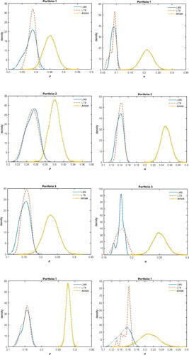
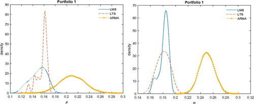
In turn, we can use the appropriately modified posteriors for both LMS and LTS. Moreover, the ARMA posterior can be easily handled using the Gibbs sampler. In Figure 5, we report marginal posterior densities of ρ and α for the empirical application of the previous section. Again, ARMA overestimates both ρ and α by a significant amount, in terms of posterior means or medians, for all four portfolios.

Fig. 5 Marginal posteriors of LMS, LTS and ARMA.

4.3 Model selection

Suppose we consider a general ARMA(p,q) model and we want to perform Bayesian Model Averaging (BMA) or compute posterior model probabilities. The critical part is to compute marginal likelihoods also known as “evidence”, With a likelihood $L(\theta ;Y)$ and a prior $p(\theta )$, ($\theta \in \Theta \subseteq {\mathbb{R}}^d$), the marginal likelihood is (17) $$M(Y)=\frac{L(\theta ;Y)p(\theta )}{p(\theta |Y)}.$$(17)

As this is an identity in θ, it holds at $\overline{\theta }$ as well (say the posterior mean or median which can be computed easily from MCMC output). Therefore, we have (18) $$\mathcal{M}(Y)=\frac{L(\overline{\theta };Y)p(\overline{\theta })}{p(\overline{\theta }|Y)}.$$(18)

Since the denominator is unknown, we can use a Laplace approximation to obtain $p(\overline{\theta }|Y)\simeq {(2\pi )}^{-d/2}|V{|}^{-1/2}$, where V is the posterior covariance matrix of θ which can be computed easily from MCMC (DiCiccio et al. 1997). If we have different models, say $m\in \left\{1,\dots ,M\right\}$ posterior model probabilities can be computed as (19) $$P_m(Y)=\frac{{\mathcal{M}}_m(Y)p({\theta }_m)}{\sum _{j=1}^m{\mathcal{M}}_j(Y)},>m\in \left\{1,\dots ,M\right\}.$$(19) assuming that model m has parameters, likelihood, and prior given, respectively, by ${\theta }_m,L_m({\theta }_m;Y),p({\theta }_m)$. Moreover, the marginal likelihood for model m is denoted ${\mathcal{M}}_m(Y)$. We report posterior model probabilities in Table 1 for portfolio 1 as results for other portfolios were nearly the same. Clearly, the lion’s share goes to ARMA(1,1) with posterior probability 0.480. In case of model selection, the model that should be selected in ARMA(1,1). The posterior probabilities for LTS were qualitatively similar but very different for ARMA models which favored ARMA(2,2) with posterior probability almost 0.99.

Table 1 Posterior model probabilities for ARMA(p,q), portfolio 1, posterior LMS results.

$q\downarrow$	$p\to$	0	1	2	3	4
0		0.00	0.119	0.1801	0.118	0.000
1		0.000	0.480	0.0079	0.000	0.000
2		0.000	0.040	0.023	0.031	0.000
3		0.000	0.000	0.000	0.000	0.000
4		0.000	0.000	0.000	0.000	0.000

Instead, if we use BMA the marginal posteriors densities of α and ρ from LMS are reported in Figure 6.

Fig. 6 BMA posteriors of α and ρ.

The qualitative conclusion remains the same in that BMA for ARMA provides quite different marginal posterior of ρ and α and⁶ seems to overestimate, again, the posterior means, and medians of these parameters.

5 Concluding remarks

In this article, we proposed Bayesian analysis of models with outliers using Bayesian implementations of Least Median of Squares (LMS) and Least Trimmed Squares (LTS) in models where the errors are independent, as well as in models where the errors follow AR or ARMA schemes. Monte Carlo evidence as well as an empirical application to financial portfolios shows that LMS and LTS produce more robust estimates for the volatility of portfolios, and that AR or ARMA tend to overestimate the parameters of AR(1) and ARMA(1,1) models. The techniques can be extended to general ARMA(p,q) models in a straightforward way.

Disclosure statement

No potential conflict of interest was reported by the author.

Notes

1 Similar ideas have been proposed by Kato (2013) who, in the context of instrumental variables models, instead of assuming a distributional assumption, he proposed a quasi-likelihood induced from conditional moment restrictions. A similar approach has been used in Chernozhukov and Hong (2003).

2 All MCMC uses 1,500,000 passes the first 500,000 of which are omitted during the burn-in phase to mitigate possible start up effects. This is, of course, excessive, and in all cases, 15,000 omitting the first 5,000 produce the same results. Initial conditions for MCMC are provided by numerical minimization of the loss function. The standard Geweke (1992) numerical performance and MCMC convergence are inspected in all cases and they are available on request.

3 This is computed in two steps. In the first step we use OLS to obtain the residuals. From the residuals we obtain ρ by regressing the residuals on their lagged values. Finally, we use the estimated value of ρ to estimate (11)(11) $$y_t=\rho y_{t-1}+{(x_t-\rho x_{t-1})}^{\prime }\beta +e_t.$$(11) by OLS.

4 In this case, all parameters are estimated simultaneously using a standard Gibbs sampler. MCMC is based on 150,000 draws and the first 50,000 are omitted in the burn-in phase.

5 It is possible to treat e₀ as unknown parameter.

6 Since BMA for ARMA favors an ARMA(2,2) reported here for ARMA method are marginal posteriors of the first order coefficients.

References

- Bissiri, P. G., C. C. Holmes, and S. G. Walker. 2016. A general framework for updating belief distributions. Journal of the Royal Statistical Society. Series B, Statistical Methodology 78 (5):1103–30. doi: 10.1111/rssb.12158.
- Chernozhukov, V., and H. Hong. 2003. An MCMC approach to classical estimation. Journal of Econometrics 115 (03):100–3. doi: 10.1016/S0304-4076(03)00100-3.
- DiCiccio, T. J., R. E. Kass, A. Raftery, and L. Wasserman. 1997. Computing Bayes factors by combining simulation and asymptotic approximations. Journal of the American Statistical Association 92 (439):903–15. doi: 10.2307/2965554.
- Geweke, J. 1992. Evaluating the accuracy of sampling-based approaches to calculating posterior moments. In Bayesian statistics, ed. J. M. Bernado, J. O. Berger, A. P. Dawid and A. F. M. Smith, vol. 4, 169–93. Oxford, UK: Clarendon Press.
- Hastings, W. K. 1970. Monte Carlo sampling methods using Markov chains and their applications. Biometrika 57 (1):97–109. doi: 10.2307/2334940.
- Kato, K. 2013. Quasi-Bayesian analysis of nonparametric instrumental variables models. The Annals of Statistics 41 (5), 2359–90. doi: 10.1214/13-AOS1150.
- Matusita, K. 1953. On the estimation by the minimum distance method. Annals of the Institute of Statistical Mathematics 5 (2):59–65. doi: 10.1007/BF02949801.
- Matusita, K. 1955. Decision rules, based on the distance, for problems of fit, two samples, and estimation. The Annals of Mathematical Statistics 26 (4):631–40. doi: 10.1214/aoms/1177728422.
- Matusita, K. 1964. Distance and decision rules. Annals of the Institute of Statistical Mathematics 16 (1):305–15. doi: 10.1007/BF02868578.
- Piradl, S., A. Shadrokh, and M. Yarmohammadi. 2021. A robust estimation method for the linear regression model parameters with correlated error terms and outliers. Journal of Applied Statistics 49 (7):1663–76. doi: 10.1080/02664763.2021.1881454.
- Raj, S., and K. K. Senthamarai. 2017. Detection of outliers in regression model for medical data. International Journal of Medical Research & Health Sciences 6 (7):2319–5886.
- Rousseeuw, P. J. 1984. Least median of squares regression. Journal of the American Statistical Association 79 (388):871–80. doi: 10.2307/2288718.
- Tierney, L. 1994. Markov chains for exploring posterior distributions. Annals of Statistics 22:1701–62. https://www.jstor.org/stable/2242477.