Decomposition of measure from symmetry for analyzing collapsed ordinal square contingency tables

Abstract

In some situations, square contingency tables with ordered categories are analyzed by considering collapsed tables where adjacent categories are combined. This study proposes measures to represent the degree of departure from symmetry using collapsed tables. The proposed measures are defined as the arithmetic mean of submeasures of each collapsed 3 × 3 table. Additionally, a theorem affirms that the value of the measure for symmetry is equal to the sum of the value of the proposed measures. Finally, examples are given.

KEYWORDS:

• Collapsed global symmetry
• conditional symmetry
• divergence
• Kullback-Leibler information
• small-size sample

1 Introduction

Data is often organized using a square contingency table with the same classifications for categorical data analysis. Examples include matched pairs data comparisons, inter-rater reliability, changes before and after treatment, and social mobility. Independence between the row and column classifications does not hold in these square contingency tables because many observations fall in or near the main diagonal cells. Then analysis focuses on the off-diagonal cells (i.e., symmetry or asymmetry of the row and column classifications) instead of independence.

Various models have been proposed to analyze the symmetry of a square contingency table (e.g., Bowker 1948; Read 1977; and McCullagh 1978). Moreover, a measure to represent the degree of departure from the model is crucial when the model of symmetry does not fit the data well (e.g., Tomizawa 1994, 1995; and Tomizawa and Saitoh 1999).

Furthermore, to simplify the interpretation in data research, analysis of ordinal square contingency tables with many dimensions are often divided into three categories (e.g., “high,” middle,” and low”). Various methods can be used to reclassify the original categories into three groups. Consequently, a comprehensive evaluation of the different collapsed patterns is reasonable when there are numerous ways to combine ordinal categories and it is difficult to decide how to choose unique cutpoints. For example, contingency tables may be collapsed into a 3 × 3 table in clinical research when analyzing data for clinical scales or laboratory data (see Shinoda et al. 2020; Aizawa, Yamamoto, and Tomizawa 2021). Additionally, social research often treats scales with ordered categories. As an example, we use the General Social Survey conducted by the National Opinion Research Center at the University of Chicago (Davern et al. 2021). Table 1 compares the frequency that low-income respondents spent a social evening with neighbors or friends in 2012 and 2016. Table 2 shows the frequency that low-income respondents suffer everyday discrimination in 2021. When the dimensions are large or the sample size is small, previous measures cannot be estimated because the sum of symmetric cells is zero. Often analysis not only compares the degree of departure from the models but also examines the relationships among models using the decomposition of a measure from symmetry. As an example, Yamamoto, Shimada, and Tomizawa (2015) proposed a measure ${\Psi }_{\mathrm{S}}$ to represent the degree of departure from symmetry (S) using collapsed a 3 × 3 table. Noting that the measure ${\Psi }_{\mathrm{S}}$ is described in detail in the next section.

Table 1 Frequency of spending evenings with friends and neighbors for low-income respondents in 2012 and 2016 from Davern et al. (2021).

	(a) In 2012
	with friends
with neighbors	(1)	(2)	(3)	(4)	(5)	(6)	(7)	Total
(1)	9	6	7	0	3	1	1	27
(2)	1	10	4	9	2	1	6	33
(3)	2	1	0	3	1	0	3	10
(4)	0	3	5	2	6	3	2	21
(5)	0	0	2	1	4	0	1	8
(6)	0	0	1	1	1	0	2	5
(7)	1	8	8	7	4	5	14	47
Total	13	28	27	23	21	10	29	151
	(b) In 2016
	with friends
with neighbors	(1)	(2)	(3)	(4)	(5)	(6)	(7)	Total
(1)	1	7	8	2	0	2	3	23
(2)	2	11	12	13	2	0	1	41
(3)	0	4	5	7	0	0	0	16
(4)	4	2	2	7	2	2	4	23
(5)	0	0	0	1	2	0	2	5
(6)	0	1	3	6	0	4	2	16
(7)	3	10	7	7	8	4	26	65
Total	10	35	37	43	14	12	38	189

Note: Status is (1) almost every day, (2) once or twice a week, (3) several times a month, (4) about once a month, (5) several times a year, (6) about once a year, and (7) never.

Table 2 Frequency of everyday discrimination of low-income respondents in 2021 from Davern et al. (2021).

	Treated as not smart
harassed	(1)	(2)	(3)	(4)	(5)	(6)	Total
(1)	0	1	0	1	2	1	5
(2)	3	0	1	0	1	0	5
(3)	2	1	6	4	1	0	14
(4)	1	0	1	4	0	3	9
(5)	3	3	5	2	6	3	22
(6)	6	9	10	12	15	50	102
Total	15	14	23	23	25	57	157

Note: Status is (1) almost every day, (2) at least once a week, (3) a few times a month, (4) a few times a year, (5) less than once a year, and (6) never.

This article proposes Kullback-Leibler (KL)-type measures to represent the degree of departure from the collapsed global symmetry (CoGS) or conditional symmetry (CS), which are denoted by ${\Psi }_{\text{CoGS}}$ or ${\Psi }_{\text{CS}}$, and demonstrates that the value of ${\Psi }_{\mathrm{S}}$ is equal to the sum of the values of ${\Psi }_{\text{CoGS}}$ and ${\Psi }_{\text{CS}}$.

2 Materials (reviews)

Consider an R × R square contingency table with the same row and column ordinal classifications. Let X and Y denote the row and column variables, respectively. Additionally, let Pr $(X=i,Y=j)=p_{ij}$ for $i=1,\dots ,R;j=1,\dots ,R$. The S model Bowker (1948) is defined as $$p_{ij}=p_{ji}\hspace{1em}(i=1,\dots ,R; j=1,\dots ,R; i\ne j).$$

Also, see Bishop, Fienberg, and Holland (1975, p.282). The global symmetry (GS) model proposed by Read (1977) is given as $${\delta }_1={\delta }_2,$$where ${\delta }_1={\sum }_{i=1}^{R-1}{\sum }_{j=i+1}^R{p}_{ij}$ and ${\delta }_2={\sum }_{j=1}^{R-1}{\sum }_{i=j+1}^R{p}_{ij}$. The CS model proposed by McCullagh (1978) is defined as $$p_{ij}=\Gamma p_{ji}\hspace{1em}(i<j).$$

Also, see Agresti (1990, p.361). A special case of this model is the S model when Γ = 1.

Tomizawa (1994) and Tomizawa, Seo, and Yamamoto (1998) proposed measures that represent the degree of departure from S for nominal square contingency tables. Incidentally, Tomizawa (1994) considered KL-type measures using the Shannon entropy and Gini concentration, while Tomizawa, Seo, and Yamamoto (1998) considered a generalization of Tomizawa’s (1994) measures using the power divergence (Cressie and Read 1984) or the diversity index (Patil and Taillie 1982). For ordinal square contingency tables, Tomizawa, Miyamoto, and Hatanaka (2001) proposed a measure to represent the degree of departure from S. Moreover, Tomizawa (1995) and Tomizawa and Saitoh (1999) considered measures representing the degree of departure from GS and CS, respectively. Tomizawa and Saitoh (1999) also gave the theorem that the measure from S is equal to the sum of the measure from GS and the measure from CS. See Appendixes A, B, and C for the measure ${\psi }_{\mathrm{S}},{\psi }_{\text{GS}}$, and ${\psi }_{\text{CS}}$ proposed by Tomizawa (1994), Tomizawa (1995), and Tomizawa and Saitoh (1999), respectively.

Here, we consider the $(R-1)(R-2)/2$ (being $(\begin{array}{c}R-1\\ 2\end{array})$) ways of collapsing the R × R original table with ordered categories into a 3 × 3 table by choosing cutpoints after the sth and tth rows and after the sth and tth columns for $1\le s<t\le R-1$. We refer to each collapsed 3 × 3 table as the T_st table ($1\le s<t\le R-1$). In the collapsed T_st table, let $G_{kl}^{(s,t)}$ denote the corresponding probability for row value $k (k=1,2,3)$ and column value $l (l=1,2,3)$. That is, $$\begin{array}{ccc}{G}_{11}^{(s,t)}=\sum _{i=1}^s\sum _{j=1}^s{p}_{ij},& G_{12}^{(s,t)}=\sum _{i=1}^s\sum _{j=s+1}^t{p}_{ij},& G_{13}^{(s,t)}=\sum _{i=1}^s\sum _{j=t+1}^R{p}_{ij},\\ G_{21}^{(s,t)}=\sum _{i=s+1}^t\sum _{j=1}^s{p}_{ij},& G_{22}^{(s,t)}=\sum _{i=s+1}^t\sum _{j=s+1}^t{p}_{ij},& G_{23}^{(s,t)}=\sum _{i=s+1}^t\sum _{j=t+1}^R{p}_{ij},\\ G_{31}^{(s,t)}=\sum _{i=t+1}^R\sum _{j=1}^s{p}_{ij},& G_{32}^{(s,t)}=\sum _{i=t+1}^R\sum _{j=s+1}^t{p}_{ij},& G_{33}^{(s,t)}=\sum _{i=t+1}^R\sum _{j=t+1}^R{p}_{ij}.\end{array}$$

Then the S model is expressed as $$G_{kl}^{(s,t)}=G_{lk}^{(s,t)}\hspace{1em}(k=1,2,3; l=1,2,3; k\ne l),$$for all s and t ($1\le s<t\le R-1$). See Yamamoto, Tahata, and Tomizawa (2012). Similarly, the CS model can be expressed as $$G_{kl}^{(s,t)}=\Gamma G_{lk}^{(s,t)}\hspace{1em}(k<l),$$ for all s and t ($1\le s<t\le R-1$). Here, consider a model defined by $${\Delta }_1^{(s,t)}={\Delta }_2^{(s,t)},$$ where ${\Delta }_1^{(s,t)}={\sum }_{k=1}^2{\sum }_{l=k+1}^3{G}_{kl}^{(s,t)}$ and ${\Delta }_2^{(s,t)}={\sum }_{l=1}^2{\sum }_{k=l+1}^3{G}_{kl}^{(s,t)}$ for all s and t ($1\le s<t\le R-1$). This model is not equivalent to the GS model. This model is referred to as the CoGS model (Yamamoto, Tahata, and Tomizawa 2012).

Assuming that $\{G_{kl}^{(s,t)}+G_{lk}^{(s,t)}>0\}$ for $1\le s<t\le R-1$ and $1\le k<l\le 3$, the measure to represent the degree of departure from S proposed by Yamamoto, Shimada, and Tomizawa (2015) can be expressed as $${\Psi }_{\mathrm{S}}=\frac{1}{\left(\begin{array}{c}R-1\\ 2\end{array}\right)}\sum _{s=1}^{R-2}\sum _{t=s+1}^{R-1}{\Psi }_{\mathrm{S}}^{(s,t)},$$where $$\begin{array}{c}{\Psi }_{\mathrm{S}}^{(s,t)}=\frac{1}{\hspace{0.17em}\log \hspace{0.17em}2}\sum _{k=1}^2\sum _{l=k+1}^3[G_{kl}^{\ast (s,t)}\hspace{0.17em}\log \hspace{0.17em}\left(\frac{G_{kl}^{\ast (s,t)}}{\left(G_{kl}^{\ast (s,t)}+G_{lk}^{\ast (s,t)}\right)/2}\right)\\ \hspace{1em}+G_{lk}^{\ast (s,t)}\hspace{0.17em}\log \hspace{0.17em}\left(\frac{G_{lk}^{\ast (s,t)}}{\left(G_{kl}^{\ast (s,t)}+G_{lk}^{\ast (s,t)}\right)/2}\right)],\\ {\Delta }^{(s,t)}=\sum _{k=1}^2\sum _{l=k+1}^3\left(G_{kl}^{(s,t)}+G_{lk}^{(s,t)}\right),\hspace{1em}{G}_{kl}^{\ast (s,t)}=\frac{G_{kl}^{(s,t)}}{{\Delta }^{(s,t)}}.\end{array}$$

It should be noted that the measure ${\Psi }_{\mathrm{S}}$ using collapsed 3 × 3 tables completely differs from the measure proposed by Tomizawa, Miyamoto, and Hatanaka (2001).

3 Measures for collapsed 3 × 3 tables

3.1 Measure of departure from CoGS

Assuming that $\{{\Delta }^{(s,t)}>0\}$ for $1\le s<t\le R-1$, consider a measure representing the degree of departure from CoGS, which is defined as $${\Psi }_{\text{CoGS}}=\frac{1}{\left(\begin{array}{c}R-1\\ 2\end{array}\right)}\sum _{s=1}^{R-2}\sum _{t=s+1}^{R-1}{\Psi }_{\text{CoGS}}^{(s,t)},$$where $$\begin{array}{c}{\Psi }_{\text{CoGS}}^{(s,t)}=\frac{1}{\hspace{0.17em}\log \hspace{0.17em}2}\sum _{k=1}^2{\Delta }_k^{\ast (s,t)}\hspace{0.17em}\log \hspace{0.17em}\left(\frac{{\Delta }_k^{\ast (s,t)}}{1/2}\right),\\ {\Delta }_1^{\ast (s,t)}=\frac{{\Delta }_1^{(s,t)}}{{\Delta }^{(s,t)}},\hspace{1em}{\Delta }_2^{\ast (s,t)}=\frac{{\Delta }_2^{(s,t)}}{{\Delta }^{(s,t)}}.\end{array}$$

The measure ${\Psi }_{\text{CoGS}}$ is between 0 and 1. ${\Psi }_{\text{CoGS}}$ has the following characteristics:

1. ${\Psi }_{\text{CoGS}}=0$ if and only if CoGS holds;

2. ${\Psi }_{\text{CoGS}}=1$ if and only if ${\Delta }_1^{(s,t)}=0$ (then ${\Delta }_2^{(s,t)}>0$) or ${\Delta }_2^{(s,t)}=0$ (then ${\Delta }_1^{(s,t)}>0$) for $1\le s<t\le R-1$.

Note that the definition of the maximum departure from CoGS can also be expressed as p_ij = 0 (then p_ji > 0) or p_ji = 0 (then p_ij > 0) for all i < j. Although the CoGS model is not equivalent to the GS model, the maximum departure has the same definition in both models.

3.2 Measure of departure from CS

Assuming that $\{{\Delta }_1^{(s,t)}>0\},\{{\Delta }_2^{(s,t)}>0\}$ and $\{G_{kl}^{(s,t)}+G_{lk}^{(s,t)}>0\}$ for $1\le s<t\le R-1$ and $1\le k<l\le 3$, a measure representing the degree of departure from CS is defined as $${\Psi }_{\text{CS}}=\frac{1}{\left(\begin{array}{c}R-1\\ 2\end{array}\right)}\sum _{s=1}^{R-2}\sum _{t=s+1}^{R-1}{\Psi }_{\text{CS}}^{(s,t)},$$where $$\begin{array}{c}{\Psi }_{\text{CS}}^{(s,t)}=\frac{1}{\hspace{0.17em}\log \hspace{0.17em}2}\sum _{k=1}^2\sum _{l=k+1}^3[G_{kl}^{\ast (s,t)}\hspace{0.17em}\log \hspace{0.17em}\left(\frac{G_{kl}^{\ast (s,t)}}{{\Delta }_1^{\ast (s,t)}\left(G_{kl}^{\ast (s,t)}+G_{lk}^{\ast (s,t)}\right)}\right)\\ \hspace{1em}+G_{lk}^{\ast (s,t)}\hspace{0.17em}\log \hspace{0.17em}\left(\frac{G_{lk}^{\ast (s,t)}}{{\Delta }_2^{\ast (s,t)}\left(G_{kl}^{\ast (s,t)}+G_{lk}^{\ast (s,t)}\right)}\right)].\end{array}$$

${\Psi }_{\text{CS}}$ is between 0 and 1. ${\Psi }_{\text{CS}}$ has the following characteristics:

1. ${\Psi }_{\text{CS}}=0$ if and only if CS holds;

2. ${\Psi }_{\text{CS}}=1$ if and only if ${\Delta }_1^{(s,t)}={\Delta }_2^{(s,t)}$ and $G_{kl}^{(s,t)}=0$ (then $G_{lk}^{(s,t)}>0$) or $G_{lk}^{(s,t)}=0$ (then $G_{kl}^{(s,t)}>0$) for $1\le s<t\le R-1$ and $1\le k<l\le 3$.

3.3 Relationships between the measures

Assuming that $\{{\Delta }_1^{(s,t)}>0\},\{{\Delta }_2^{(s,t)}>0\}$ and $\{G_{kl}^{(s,t)}+G_{lk}^{(s,t)}>0\}$ for $1\le s<t\le R-1$ and $1\le k<l\le 3$, the following theorems are obtained.

Theorem 1.

The value of ${\Psi }_{\mathrm{S}}$ is equal to the sum of the value of ${\Psi }_{\text{CoGS}}$ and the value of ${\Psi }_{\text{CS}}$.

Proof.

Consider that the sum of the value of ${\Psi }_{\text{CoGS}}$ and the value of ${\Psi }_{\text{CS}}$ can be expressed as $${\Psi }_{\text{CoGS}}+{\Psi }_{\text{CS}}=\frac{1}{\left(\begin{array}{c}R-1\\ 2\end{array}\right)}\sum _{s=1}^{R-2}\sum _{t=s+1}^{R-1}\left({\Psi }_{\text{CoGS}}^{(s,t)}+{\Psi }_{\text{CS}}^{(s,t)}\right),$$where $$\begin{array}{c}{\Psi }_{\text{CoGS}}^{(s,t)}+{\Psi }_{\text{CS}}^{(s,t)}=\frac{1}{\hspace{0.17em}\log \hspace{0.17em}2}\sum _{k=1}^2\sum _{l=k+1}^3[\mathrm{}\mathrm{}{G}_{kl}^{\ast (s,t)}\left\{\hspace{0.17em}\log \hspace{0.17em}\left(\frac{{\Delta }_1^{\ast (s,t)}}{1/2}\right)+\hspace{0.17em}\log \hspace{0.17em}\left(\mathrm{}\frac{G_{kl}^{\ast (s,t)}}{{\Delta }_1^{\ast (s,t)}\left(G_{kl}^{\ast (s,t)}+G_{lk}^{\ast (s,t)}\right)}\mathrm{}\right)\mathrm{}\right\}\\ \hspace{1em}+G_{lk}^{\ast (s,t)}\left\{\hspace{0.17em}\log \hspace{0.17em}\left(\frac{{\Delta }_2^{\ast (s,t)}}{1/2}\right)+\hspace{0.17em}\log \hspace{0.17em}\left(\frac{G_{lk}^{\ast (s,t)}}{{\Delta }_2^{\ast (s,t)}\left(G_{kl}^{\ast (s,t)}+G_{lk}^{\ast (s,t)}\right)}\right)\right\}]\\ =\frac{1}{\hspace{0.17em}\log \hspace{0.17em}2}\sum _{k=1}^2\sum _{l=k+1}^3[G_{kl}^{\ast (s,t)}\hspace{0.17em}\log \hspace{0.17em}\left(\frac{G_{kl}^{\ast (s,t)}}{\left(G_{kl}^{\ast (s,t)}+G_{lk}^{\ast (s,t)}\right)/2}\right)\\ \hspace{1em}+G_{lk}^{\ast (s,t)}\hspace{0.17em}\log \hspace{0.17em}\left(\frac{G_{lk}^{\ast (s,t)}}{\left(G_{kl}^{\ast (s,t)}+G_{lk}^{\ast (s,t)}\right)/2}\right)].\end{array}$$

Consequently, ${\Psi }_{\text{CoGS}}^{(s,t)}+{\Psi }_{\text{CS}}^{(s,t)}={\Psi }_{\mathrm{S}}^{(s,t)}$. Then ${\Psi }_{\text{CoGS}}+{\Psi }_{\text{CS}}={\Psi }_{\mathrm{S}}$. □

From Theorem 1, ${\Psi }_{\text{CS}}$ is expressed as ${\Psi }_{\text{CS}}={\Psi }_{\mathrm{S}}-{\Psi }_{\text{CoGS}}$. Therefore, the measure ${\Psi }_{\text{CS}}$ should indicate the degree of departure from S without the influence of the degree of departure from CoGS. That is, ${\Psi }_{\text{CS}}$ indicates the degree of departure from S under the condition that there is a structure of CoGS.

Under Theorem 1, Theorem 2 can be obtained considering ${\Psi }_{\text{CS}}\ge 0$.

Theorem 2.

The value of ${\Psi }_{\mathrm{S}}$ is greater than or equal to the value of ${\Psi }_{\text{CoGS}}$. The equality holds if and only if there is a conditional symmetry structure in the R × R table.

From $0\le {\Psi }_{\mathrm{S}}\le 1$ and $0\le {\Psi }_{\text{CoGS}}<1$ (note that ${\Psi }_{\text{CoGS}}\ne 1$ due to the assumption that $\{{\Delta }^{(s,t)}>0\}$), we see that $0\le {\Psi }_{\text{CS}}\le 1$. Therefore, (i) ${\Psi }_{\mathrm{S}}={\Psi }_{\text{CoGS}}$ if and only if there is a structure of CS (${\Psi }_{\text{CS}}=0$), and (ii) ${\Psi }_{\mathrm{S}}=1$ and ${\Psi }_{\text{CoGS}}=0$ if and only if ${\Psi }_{\text{CS}}=1$. Moreover, according to the KL information, ${\Psi }_{\text{CS}}$ represents the degree of departure from CS, and the degree of departure increases as the value of ${\Psi }_{\text{CS}}$ increases. That is, ${\Psi }_{\text{CS}}$ is the difference between the degree of departure from S and that from CoGS.

4 Approximate confidence interval for measure

Let n_ij denote the observed frequency in the ith row and jth column of the table ($i=1,\dots ,R; j=1,\dots ,R$). The sample version of ${\Psi }_{\text{CoGS}}$ (${\Psi }_{\text{CS}}$), which is, ${\widehat{\Psi }}_{\text{CoGS}}$ (${\widehat{\Psi }}_{\text{CS}}$), is given by ${\Psi }_{\text{CoGS}}$ where $\left\{p_{ij}\right\}$ is replaced by $\left\{{\widehat{p}}_{ij}\right\}$. Here, ${\widehat{p}}_{ij}=n_{ij}/n$ and $n=\sum \sum n_{ij}$. Assuming that $\left\{n_{ij}\right\}$ results from full multinomial sampling, we consider the approximate standard error for ${\widehat{\Psi }}_{\text{CoGS}}$ and a large-sample confidence interval for ${\Psi }_{\text{CoGS}}$. Using the delta method, $\sqrt[]{n}({\widehat{\Psi }}_{\text{CoGS}}-{\Psi }_{\text{CoGS}})$ has an asymptotically (as $n\to \infty$) normal distribution with a mean of zero and a variance ${\sigma }^2[{\Psi }_{\text{CoGS}}]$. See Appendixes D and E for details of ${\sigma }^2[{\Psi }_{\text{CoGS}}]$ and ${\sigma }^2[{\Psi }_{\text{CS}}]$.

Let ${\widehat{\sigma }}^2[{\Psi }_{\text{CoGS}}]$ denote ${\sigma }^2[{\Psi }_{\text{CoGS}}]$ where $\left\{p_{ij}\right\}$ is replaced by $\left\{{\widehat{p}}_{ij}\right\}$. Then $\widehat{\sigma }[{\Psi }_{\text{CoGS}}]/\sqrt[]{n}$ is an estimated approximate standard error for ${\widehat{\Psi }}_{\text{CoGS}}$, and ${\widehat{\Psi }}_{\text{CoGS}}\pm z_{p/2}\widehat{\sigma }[{\Psi }_{\text{CoGS}}]/\sqrt[]{n}$ is an approximate $100(1-p)$ percent confidence interval for ${\Psi }_{\text{CoGS}}$, where $z_{p/2}$ is the $100(1-p/2)$th percentile of the standard normal distribution.

5 Examples

Table 1 shows the cross classifications of the respondents’ opinions about spending the evening with friends or neighbors in 2012 and 2016. Here, we considered low-income respondents (annual income under $15,000). The response categories are (1) “almost every day,” (2) “once or twice a week,” (3) several times a month,” (4) “about once a month,” (5) “several times a year,” (6) “about once a year,” and (7) “never.” The degree of departure from CS between Table 1a,b is compared using ${\Psi }_{\text{CS}}$. Table 3 shows that the estimated values of ${\Psi }_{\text{CS}}$ are 0.100 for Table 1a and 0.133 for Table 1b. Although the confidence intervals overlap, the degree of departure from CS is greater in Table 1b than in Table 1a. By contrast, the existing measure ${\psi }_{\text{CS}}$ cannot be estimated, because the sum of the symmetric cells is 0.

Table 3 Estimates of measures ${\Psi }_{\text{CS}},{\Psi }_{\text{CoGS}}$, and ${\Psi }_{\mathrm{S}}$, approximate standard errors, and 95% confidence intervals applied to the data in Tables 1 and 2.

Application	Measure	Estimated measure	Standard error	Confidence interval
Table 1a	${\Psi }_{\text{CS}}$	0.100	0.036	$(0.030,0.171)$
	${\Psi }_{\text{CoGS}}$	0.020	0.009	$(0.002,0.037)$
	${\Psi }_{\mathrm{S}}$	0.120	0.042	$(0.038,0.202)$
Table 1b	${\Psi }_{\text{CS}}$	0.133	0.037	$(0.060,0.207)$
	${\Psi }_{\text{CoGS}}$	0.047	0.020	$(0.007,0.087)$
	${\Psi }_{\mathrm{S}}$	0.180	0.052	$(0.078,0.283)$
Table 2	${\Psi }_{\text{CS}}$	0.037	0.020	$(-0.003,0.077)$
	${\Psi }_{\text{CoGS}}$	0.327	0.091	$(0.149,0.506)$
	${\Psi }_{\mathrm{S}}$	0.364	0.088	$(0.192,0.536)$

Table 2 describes the cross classifications of respondent’s opinions regarding everyday discrimination (people act as if they think the respondent is not smart; the respondent is harassed) in 2021. Here, we considered low-income respondents (annual income under $8,000). The response categories are (1) “almost every day,” (2) “at least once a week,” (3) “a few times a month,” (4) “a few times a year,” (5) “less than once a year,” and (6) “never.” The confidence intervals for ${\Psi }_{\mathrm{S}}$ and ${\Psi }_{\text{CoGS}}$ do not include zero (see Table 3), indicating that S and CoGS do not have a structure. By contrast, the confidence interval for ${\Psi }_{\text{CS}}$ includes zero (see Table 3), suggesting that CS has a structure in the table. Moreover, Theorem 1 shows that the lack of structure of the S model is due to the lack of structure of the CoGS model rather than that of the CS model. Thus, the CS model may reveal that respondents treated as not smart are harassed more often in daily life. By contrast, existing measures ${\psi }_{\text{CS}}$ and ${\psi }_{\mathrm{S}}$ cannot be estimated because the sum of symmetric cells is 0.

6 Discussion

The value of ${\Psi }_{\text{CS}}$ increases as the difference between the degree of departure from S and that from CoGS increases. This is especially pronounced as the degree of departure from S increases while that from GS decreases. The value of ${\Psi }_{\text{CS}}$ reaches the maximum (= 1) when the degree of departure from S is maximized (= 1) and that from CoGS is minimized (= 0). Therefore, ${\Psi }_{\text{CS}}$ is useful to visualize the degree of departure from CS on the complete asymmetry with the CoGS structure.

It is also meaningful to consider collapsed 3 × 3 tables only when the original square contingency table has ordered categories because the collapsed tables are obtained by combining adjacent categories. The measure in square ordinal tables should depend on the listing order of the categories. The proposed measures are not invariant under arbitrary similar permutations of row and column categories, except for the reverse order. Moreover, whether the submeasures of the collapsed tables are invariant does not matter because each collapsed 3 × 3 table obtained from an original square table is unique.

We show that even if the estimated measures of ${\psi }_{\text{CS}}$ and ${\psi }_{\mathrm{S}}$ cannot be calculated because the sum of symmetric cells is zero in the original table, the estimated measures of ${\Psi }_{\text{CS}}$ and ${\Psi }_{\mathrm{S}}$ can be calculated in some cases. This property may be useful, especially for a small-size sample or a large dimension of R.

It should be noted that Yamamoto, Shimada, and Tomizawa (2015) gave the power divergence-type (including the KL) measure to represent the degree of departure from S. However, using the power divergence does not provide a result similar to Theorem 1. The CoGS and CS models do not impose restrictions on the diagonal cell probabilities. Therefore, it seems natural that the proposed measures and their ranges are independent of the diagonal cell probabilities.

The asymptotic normal distribution of $\sqrt[]{n}({\widehat{\Psi }}_{\text{CoGS}}-{\Psi }_{\text{CoGS}})$ is not applicable when ${\Psi }_{\text{CoGS}}=0$ or ${\Psi }_{\text{CoGS}}=1$ because ${\sigma }^2[{\Psi }_{\text{CoGS}}]=0$. Additionally, the asymptotic normal distribution of ${\Psi }_{\text{CS}}$ is not applicable for the same reason. The above issues are common to existing measures not only the proposed measures. As an example to address these issues, we conducted Monte Carlo simulations using the proposed measure (see Appendix F). In the simulations, four contingency tables were assumed with true values of the proposed measure ranging from 0.000 to 0.090, and the sampling distribution of the proposed measures were visualized in a histogram. When the true value of the measure is 0.000, the asymptotic normal distribution may be difficult to be applicable. However, with a large enough sample, the asymptotic normal distribution may be applicable even if the true value of the measure is close to 0.000. Therefore, we would consider using resampling methods or Bayesian methods when the true values of measures are very close to 0.000 or 1.000, or the small sample size. As an example of a Bayesian approach, Momozaki et al. (2021) considered new estimators of measures that can reduce the bias and mean squared error even without a sufficient sample size using the Bayesian estimators of cell probabilities.

7 Conclusion

Considering collapsed 3 × 3 tables can simplify the interpretation. If determining how to choose unique cutpoints is difficult, then it is reasonable to evaluate the collapsed square contingency tables for various patterns. Thus, we consider that all ${\Psi }_{\text{CoGS}}^{(s,t)}$ (${\Psi }_{\text{CS}}^{(s,t)}$) are combined at the same weights $1/(\begin{array}{c}R-1\\ 2\end{array})$. The proposed measures are useful for comparing the degrees of departure from S, CoGS, and CS in several tables since the proposed measures always range between 0 and 1 and are independent of the sample size and the dimension R. The proposed theorems are also meaningful to comprehend the relation of these three measures.

Acknowledgments

The authors would like to thank the referees for their comments.

Additional information

Funding

This work was supported by a Grant-in-Aid for Research Activity Start-up from JSPS MEXT KAKENHI (Number 21463537).

Appendix A

Appendix A

Assuming that $\{p_{ij}+p_{ji}>0\}$ for $1\le i<j\le R$, the measure to represent the degree of departure from the symmetry proposed by Tomizawa (1994) is given as $${\psi }_{\mathrm{S}}=\frac{1}{\hspace{0.17em}\log \hspace{0.17em}2}\sum _{i=1}^{R-1}\sum _{j=i+1}^R\left[p_{ij}^{\ast }\hspace{0.17em}\log \hspace{0.17em}\left(\frac{p_{ij}^{\ast }}{(p_{ij}^{\ast }+p_{ji}^{\ast })/2}\right)+p_{ji}^{\ast }\hspace{0.17em}\log \hspace{0.17em}\left(\frac{p_{ji}^{\ast }}{(p_{ij}^{\ast }+p_{ji}^{\ast })/2}\right)\right],$$where $$\delta =\sum _{i=1}^{R-1}\sum _{j=i+1}^R\left(p_{ij}+p_{ji}\right), p_{ji}^{\ast }=p_{ji}/\delta .$$

Appendix B

Appendix B

Assuming that ${\delta }_1+{\delta }_2>0$, the measure to represent the degree of departure from the global symmetry proposed by Tomizawa (1995) is given as $${\psi }_{\text{GS}}=\frac{1}{\log 2}{\displaystyle \sum _{i=1}^2{\delta }_i^{\ast }}\log \left(\frac{{\delta }_i^{\ast }}{1/2}\right),Z{\psi }_{\text{GS}}=\frac{1}{\log 2}{\displaystyle \sum _{i=1}^2{\delta }_i^{\ast }}\log \left(\frac{{\delta }_i^{\ast }}{1/2}\right),$$where $${\delta }_1=\sum _{i=1}^{R-1}\sum _{j=i+1}^R{p}_{ij}, {\delta }_2=\sum _{j=1}^{R-1}\sum _{i=j+1}^R{p}_{ij}, {\delta }_i^{\ast }=\frac{{\delta }_i}{\delta }.$$

Appendix C

Appendix C

Assuming that ${\delta }_1>0,{\delta }_2>0$ and $\{p_{ij}+p_{ji}>0\}$ for $1\le i<j\le R$, the measure to represent the degree of departure from the conditional symmetry proposed by Tomizawa and Saitoh (1999) is given as $${\psi }_{\text{CS}}=\frac{1}{\hspace{0.17em}\log \hspace{0.17em}2}\sum _{i=1}^{R-1}\sum _{j=i+1}^R\left[p_{ij}^{\ast }\hspace{0.17em}\log \hspace{0.17em}\left(\frac{p_{ij}^{\ast }}{{\delta }_1^{\ast }(p_{ij}^{\ast }+p_{ji}^{\ast })}\right)+p_{ji}^{\ast }\hspace{0.17em}\log \hspace{0.17em}\left(\frac{p_{ji}^{\ast }}{{\delta }_2^{\ast }(p_{ij}^{\ast }+p_{ji}^{\ast })}\right)\right].$$

Appendix D

Appendix D

Using the delta method, $\sqrt[]{n}({\widehat{\Psi }}_{\text{CoGS}}-{\Psi }_{\text{CoGS}})$ has an asymptotic variance ${\sigma }^2[{\Psi }_{\text{CoGS}}]$ given as $${\sigma }^2\left[{\Psi }_{\text{CoGS}}\right]=\sum _{i=1}^{R-1}\sum _{j=i+1}^R\left(p_{ij}{W}_{ij}^2+p_{ji}{V}_{ji}^2\right)-{\left[\sum _{i=1}^{R-1}\sum _{j=i+1}^R\left(p_{ij}{W}_{ij}+p_{ji}{V}_{ji}\right)\right]}^2,$$where $$\begin{array}{c}{W}_{ij}=\frac{1}{\left(\begin{array}{c}R-1\\ 2\end{array}\right)}\sum _{s=1}^{R-2}\sum _{t=s+1}^{R-1}I(\ast 1)\frac{1}{\hspace{0.17em}\log \hspace{0.17em}2}\frac{{\Delta }_2^{(s,t)}}{{({\Delta }^{(s,t)})}^2}\log \hspace{0.17em}\left(\frac{{\Delta }_1^{(s,t)}}{{\Delta }_2^{(s,t)}}\right),\\ V_{ji}=\frac{1}{\left(\begin{array}{c}R-1\\ 2\end{array}\right)}\sum _{s=1}^{R-2}\sum _{t=s+1}^{R-1}I(\ast 2)\frac{1}{\hspace{0.17em}\log \hspace{0.17em}2}\frac{{\Delta }_1^{(s,t)}}{{({\Delta }^{(s,t)})}^2}\log \hspace{0.17em}\left(\frac{{\Delta }_2^{(s,t)}}{{\Delta }_1^{(s,t)}}\right),\\ \ast 1=(1\le i\le s,s+1\le j\le t)\cup (1\le i\le s,t+1\le j\le R)\\ \hspace{1em}\cup (s+1\le i\le t,t+1\le j\le R),\\ \ast 2=(1\le j\le s,s+1\le i\le t)\cup (1\le j\le s,t+1\le i\le R)\\ \hspace{1em}\cup (s+1\le j\le t,t+1\le i\le R),\end{array}$$ and $I(·)$ is the indicator function.

Appendix E

Appendix E

Using the delta method, $\sqrt[]{n}({\widehat{\Psi }}_{\text{CS}}-{\Psi }_{\text{CS}})$ has an asymptotic variance ${\sigma }^2[{\Psi }_{\text{CS}}]$ given as $${\sigma }^2\left[{\Psi }_{\text{CS}}\right]=\sum _{i=1}^{R-1}\sum _{j=i+1}^R\left(p_{ij}{A}_{ij}^2+p_{ji}{B}_{ji}^2\right)-{\left[\sum _{i=1}^{R-1}\sum _{j=i+1}^R\left(p_{ij}{A}_{ij}+p_{ji}{B}_{ji}\right)\right]}^2,$$where $$\begin{array}{c}{A}_{ij}=\frac{1}{\left(\begin{array}{c}R-1\\ 2\end{array}\right)}\sum _{s=1}^{R-2}\sum _{t=s+1}^{R-1}\frac{1}{{({\Delta }^{(s,t)})}^2\hspace{0.17em}\log \hspace{0.17em}2}[I(\ast \ast 1)C_{12}^{(s,t)}-I(\ast \ast 2)D_{12}^{(s,t)}+I(\ast \ast 3)C_{13}^{(s,t)}\\ \hspace{1em}-I(\ast \ast 4)D_{13}^{(s,t)}+I(\ast \ast 5)C_{23}^{(s,t)}-I(\ast \ast 6)D_{23}^{(s,t)}],\\ B_{ij}=\frac{1}{\left(\begin{array}{c}R-1\\ 2\end{array}\right)}\sum _{s=1}^{R-2}\sum _{t=s+1}^{R-1}\frac{1}{{({\Delta }^{(s,t)})}^2\hspace{0.17em}\log \hspace{0.17em}2}[I(\ast \ast 7)E_{12}^{(s,t)}-I(\ast \ast 8)F_{12}^{(s,t)}+I(\ast \ast 9)E_{13}^{(s,t)}\\ \hspace{1em}-I(\ast \ast 10)F_{13}^{(s,t)}+I(\ast \ast 11)E_{23}^{(s,t)}-I(\ast \ast 12)F_{23}^{(s,t)}],\\ C_{kl}^{(s,t)}={\Delta }^{(s,t)}\hspace{0.17em}\log \hspace{0.17em}\left(\frac{{\Delta }^{(s,t)}{G}_{kl}^{(s,t)}}{{\Delta }_1^{(s,t)}(G_{kl}^{(s,t)}+G_{lk}^{(s,t)})}\right)-G_{kl}^{(s,t)}\left\{\hspace{0.17em}\log \hspace{0.17em}\left(\frac{{\Delta }^{(s,t)}{G}_{kl}^{(s,t)}}{{\Delta }_1^{(s,t)}(G_{kl}^{(s,t)}+G_{lk}^{(s,t)})}\right)-1\right\}\\ \hspace{1em}-G_{lk}^{(s,t)}\left\{\hspace{0.17em}\log \hspace{0.17em}\left(\frac{{\Delta }^{(s,t)}{G}_{lk}^{(s,t)}}{{\Delta }_2^{(s,t)}(G_{kl}^{(s,t)}+G_{lk}^{(s,t)})}\right)-1\right\}-\frac{{\Delta }^{(s,t)}{G}_{kl}^{(s,t)}}{{\Delta }_1^{(s,t)}},\\ D_{kl}^{(s,t)}=G_{kl}^{(s,t)}\left\{\hspace{0.17em}\log \hspace{0.17em}\left(\frac{{\Delta }^{(s,t)}{G}_{kl}^{(s,t)}}{{\Delta }_1^{(s,t)}(G_{kl}^{(s,t)}+G_{lk}^{(s,t)})}\right)-1\right\}+G_{lk}^{(s,t)}\left\{\hspace{0.17em}\log \hspace{0.17em}\left(\frac{{\Delta }^{(s,t)}{G}_{lk}^{(s,t)}}{{\Delta }_2^{(s,t)}(G_{kl}^{(s,t)}+G_{lk}^{(s,t)})}\right)-1\right\}\\ \hspace{1em}+\frac{{\Delta }^{(s,t)}{G}_{kl}^{(s,t)}}{{\Delta }_1^{(s,t)}},\\ E_{kl}^{(s,t)}={\Delta }^{(s,t)}\hspace{0.17em}\log \hspace{0.17em}\left(\frac{{\Delta }^{(s,t)}{G}_{lk}^{(s,t)}}{{\Delta }_2^{(s,t)}(G_{kl}^{(s,t)}+G_{lk}^{(s,t)})}\right)-G_{kl}^{(s,t)}\left\{\hspace{0.17em}\log \hspace{0.17em}\left(\frac{{\Delta }^{(s,t)}{G}_{kl}^{(s,t)}}{{\Delta }_1^{(s,t)}(G_{kl}^{(s,t)}+G_{lk}^{(s,t)})}\right)-1\right\}\\ \hspace{1em}-G_{lk}^{(s,t)}\left\{\hspace{0.17em}\log \hspace{0.17em}\left(\frac{{\Delta }^{(s,t)}{G}_{lk}^{(s,t)}}{{\Delta }_2^{(s,t)}(G_{kl}^{(s,t)}+G_{lk}^{(s,t)})}\right)-1\right\}-\frac{{\Delta }^{(s,t)}{G}_{lk}^{(s,t)}}{{\Delta }_2^{(s,t)}},\\ F_{kl}^{(s,t)}=G_{kl}^{(s,t)}\left\{\hspace{0.17em}\log \hspace{0.17em}\left(\frac{{\Delta }^{(s,t)}{G}_{kl}^{(s,t)}}{{\Delta }_1^{(s,t)}(G_{kl}^{(s,t)}+G_{lk}^{(s,t)})}\right)-1\right\}+G_{lk}^{(s,t)}\left\{\hspace{0.17em}\log \hspace{0.17em}\left(\frac{{\Delta }^{(s,t)}{G}_{lk}^{(s,t)}}{{\Delta }_2^{(s,t)}(G_{kl}^{(s,t)}+G_{lk}^{(s,t)})}\right)-1\right\}\\ \hspace{1em}+\frac{{\Delta }^{(s,t)}{G}_{lk}^{(s,t)}}{{\Delta }_2^{(s,t)}},\end{array}$$ $$\begin{array}{c}\ast \ast 1=(1\le i\le s,s+1\le j\le t),\\ \ast \ast 2=(1\le i\le s,t+1\le j\le R)\cup (s+1\le i\le t,t+1\le j\le R),\\ \ast \ast 3=(1\le i\le s,t+1\le j\le R),\\ \ast \ast 4=(1\le i\le s,s+1\le j\le t)\cup (s+1\le i\le t,t+1\le j\le R),\\ \ast \ast 5=(s+1\le i\le t,t+1\le j\le R),\\ \ast \ast 6=(1\le i\le s,s+1\le j\le t)\cup (1\le i\le s,t+1\le j\le R),\\ \ast \ast 7=(1\le j\le s,s+1\le i\le t),\\ \ast \ast 8=(1\le j\le s,t+1\le i\le R)\cup (s+1\le j\le t,t+1\le i\le R),\\ \ast \ast 9=(1\le j\le s,t+1\le i\le R),\\ \ast \ast 10=(1\le j\le s,s+1\le i\le t)\cup (s+1\le j\le t,t+1\le i\le R),\\ \ast \ast 11=(s+1\le j\le t,t+1\le i\le R),\\ \ast \ast 12=(1\le j\le s,s+1\le i\le t)\cup (1\le j\le s,t+1\le i\le R),\end{array}$$ and $I(·)$ is the indicator function.

Appendix F

Appendix F

To confirm the sampling distribution of the proposed measures, we conducted Monte Carlo simulations. As a 6 × 6 table, we assumed random sampling by a multinomial random number based on the structures of probabilities in Table F1a–F1d. The sample size was considered $n=180,360,1,800$ (i.e., $\text{sparseness} \text{index}=5,10,50$). Each simulation studies were performed based on 1,000 trials.

The true values of both proposed measures were ${\Psi }_{\text{CoGS}}={\Psi }_{\text{CS}}=0.000$ in Table F1a, ${\Psi }_{\text{CoGS}}=0.027$ and ${\Psi }_{\text{CS}}=0.022$ in Table F1b, ${\Psi }_{\text{CoGS}}=0.059$ and ${\Psi }_{\text{CS}}=0.061$ in Table F1c, ${\Psi }_{\text{CoGS}}=0.087$ and ${\Psi }_{\text{CS}}=0.092$ in Table F1d.

Then, Figures F1–F4 represented the sampling distributions. Figure F1 (the true values are 0.000) showed that the sampling distributions of the proposed measures were not normal centered at the estimates, as expected. Figure F2 (the true values are 0.022, 0.027) showed that the asymptotic normal distribution could be applicable with a large enough sample. Furthermore, if the true value was greater than about 0.060, the sampling distribution was found to be almost normally centered.

Therefore, we must be careful using asymptotic distributions when the true value of a measure is expected to be 0.000 and/or the sample size is not large enough.

Fig. F1 The sampling distribution obtained from the structure of probabilities in Table F1a.

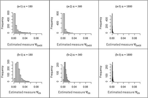
Fig. F2 The sampling distribution obtained from the structure of probabilities in Table F1b.

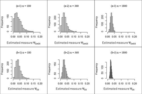
Fig. F3 The sampling distribution obtained from the structure of probabilities in Table F1c.

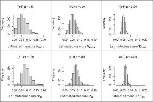
Fig. F4 The sampling distribution obtained from the structure of probabilities in Table F1d.

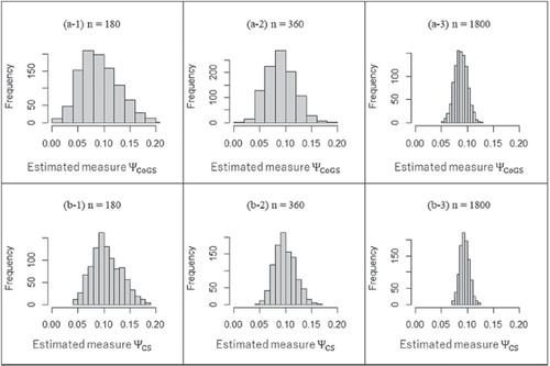
Table F1 Patterns of probability structure in a square contingency table.

(a)	1	2	3	4	5	6
1	0.0278	0.0278	0.0278	0.0278	0.0278	0.0278
2	0.0278	0.0278	0.0278	0.0278	0.0278	0.0278
3	0.0278	0.0278	0.0278	0.0278	0.0278	0.0278
4	0.0278	0.0278	0.0278	0.0278	0.0278	0.0278
5	0.0278	0.0278	0.0278	0.0278	0.0278	0.0278
6	0.0278	0.0278	0.0278	0.0278	0.0278	0.0278
(b)	1	2	3	4	5	6
1	0.0244	0.0244	0.0244	0.0244	0.0488	0.0976
2	0.0244	0.0244	0.0244	0.0244	0.0244	0.0488
3	0.0244	0.0244	0.0244	0.0244	0.0244	0.0244
4	0.0244	0.0244	0.0244	0.0244	0.0244	0.0244
5	0.0244	0.0244	0.0244	0.0244	0.0244	0.0244
6	0.0244	0.0244	0.0244	0.0244	0.0244	0.0244
(c)	1	2	3	4	5	6
1	0.0192	0.0192	0.0192	0.0192	0.0769	0.1154
2	0.0385	0.0192	0.0192	0.0192	0.0192	0.0769
3	0.0192	0.0385	0.0192	0.0192	0.0192	0.0192
4	0.0192	0.0192	0.0385	0.0192	0.0192	0.0192
5	0.0192	0.0192	0.0192	0.0385	0.0192	0.0192
6	0.0192	0.0192	0.0192	0.0192	0.0385	0.0192
(d)	1	2	3	4	5	6
1	0.0179	0.0179	0.0179	0.0179	0.0714	0.1786
2	0.0357	0.0179	0.0179	0.0179	0.0179	0.0714
3	0.0179	0.0357	0.0179	0.0179	0.0179	0.0179
4	0.0179	0.0179	0.0357	0.0179	0.0179	0.0179
5	0.0179	0.0179	0.0179	0.0357	0.0179	0.0179
6	0.0179	0.0179	0.0179	0.0179	0.0357	0.0179

References

- Agresti A. 1990. Categorical data analysis. New York: John Wiley.
- Aizawa, M., K. Yamamoto, and S. Tomizawa. 2021. Measure of departure from average marginal homogeneity for the analysis of collapsed ordinal square contingency tables. Biometrical Letters 58 (1):81–94. doi: 10.2478/bile-2021-0006.
- Bishop Y. M. M., Fienberg S. E., and Holland P. W. 1975. Discrete multivariate analysis: Theory and practice.Cambridge: The MIT Press.
- Bowker, A. H. 1948. A test for symmetry in contingency tables. Journal of the American Statistical Association 43 (244):572–4. 18123073 doi: 10.1080/01621459.1948.10483284.
- Cressie, N, and T. R. Read. 1984. Multinomial goodness-of-fit tests. Journal of the Royal Statistical Society: Series B (Methodological) 46 (3):440–64. doi: 10.1111/j.2517-6161.1984.tb01318.x.
- Davern M., Bautista R., Freese J., Morgan S. L., and Smith T. W., Bautista R., Freese J., Morgan S. L., and Smith T. W., 2021. General Social Surveys, 1972-2021 Cross-section [machine-readable data file, 68,846 cases]. Principal Investigator, Davern, M.; Co-Principal Investigators, Bautista, R., Freese, J., Morgan, S.L., and Smith, T.W.; Sponsored by National Science Foundation.-NORC ed.- Chicago: NORC at the University of Chicago [producer and distributor]. Data accessed from the GSS Data Explorer website at gssdataexplorer.norc.org.
- Mccullagh, P. 1978. A class of parametric models for the analysis of square contingency tables with ordered categories. Biometrika 65 (2):413–8. doi: 10.1093/biomet/65.2.413.
- Momozaki T., Cho K., Nakagawa T., and Tomizawa S. 2021. Estimation of measures for two-way contingency tables using the Bayesian estimators. arXiv preprint, https://arxiv.org/abs/2109.09339.
- Patil, G. P., and C. Taillie. 1982. Diversity as a concept and its measurement. Journal of the American Statistical Association 77 (379):548–61. doi: 10.1080/01621459.1982.10477845.
- Read, C. B. 1977. Partitioning chi-squape in contingency tables: A teaching approach. Communications in Statistics- Theory and Methods 6 (6):553–62. doi: 10.1080/03610927708827513.
- Shinoda, S., K. Yamamoto, K. Tahata, and S. Tomizawa. 2020. A measure of asymmetry for ordinal square contingency tables with an application to modified LANZA score data. Journal of Applied Statistics 47 (7):1251–60. 35707026 doi: 10.1080/02664763.2019.1673325.
- Tomizawa, S. 1994. Two kinds of measures of departure from symmetry in square contingency tables having nominal categories. Statistica Sinica 4 (1):325–34.
- Tomizawa, S. 1995. Measures of departure from global symmetry for square contingency tables with ordered categories. Behaviormetrika 22 (1):91–8. doi: 10.2333/bhmk.22.91.
- Tomizawa, S., N. Miyamoto, and Y. Hatanaka. 2001. Theory and methods: Measure of asymmetry for square contingency tables having ordered categories. Australian & New Zealand Journal of Statistics 43 (3):335–49. doi: 10.1111/1467-842X.00180.
- Tomizawa, S., and K. Saitoh. 1999. Kullback-Leibler information type measure of departure from conditional symmetry and decomposition of measure from symmetry for contingency tables. Calcutta Statistical Association Bulletin 49 (1-2):31–40. doi: 10.1177/0008068319990103.
- Tomizawa, S., T. Seo, and H. Yamamoto. 1998. Power-divergence-type measure of departure from symmetry for square contingency tables that have nominal categories. Journal of Applied Statistics 25 (3):387–98. doi: 10.1080/02664769823115.
- Yamamoto, K., F. Shimada, and S. Tomizawa. 2015. Measure of departure from symmetry for the analysis of collapsed square contingency tables with ordered categories. Journal of Applied Statistics 42 (4):866–75. doi: 10.1080/02664763.2014.993362.
- Yamamoto, K., K. Tahata, and S. Tomizawa. 2012. Some symmetry models for the analysis of collapsed square contingency tables with ordered categories. Calcutta Statistical Association Bulletin 64 (1-2):21–36. doi: 10.1177/0008068320120102.
Appendix A
Assuming that for
, the measure to represent the degree of departure from the symmetry proposed by Tomizawa (Citation1994) is given as
where
Appendix B
Assuming that , the measure to represent the degree of departure from the global symmetry proposed by Tomizawa (Citation1995) is given as
Appendix C
Assuming that and
for
, the measure to represent the degree of departure from the conditional symmetry proposed by Tomizawa and Saitoh (Citation1999) is given as
Appendix D
Using the delta method, has an asymptotic variance
given as
and
is the indicator function.
Appendix E