Extended Glivenko—Cantelli theorem for simple random sampling without replacement from a finite population

Abstract

In this study, we consider the rate of uniform almost sure convergence of the empirical distribution function for simple random sampling without replacement from a finite population. Utilizing Hoeffding’s inequality for simple random sampling without replacement, this study extends the classical Glivenko—Cantelli theorem for the empirical distribution function for samples from a finite population. Our numerical simulation results are consistent with theoretical results.

KEYWORDS:

• Rate of convergence
• Glivenko—Cantelli theorem
• Hoeffding’s inequality
• empirical distribution function
• finite population
• simple random sampling without replacement

1 Introduction

Empirical distribution functions and empirical processes form a major research topic in modern mathematical statistics. In statistical analysis, many statistics such as sample means, sample quantiles, M–estimators, and L–estimators can be expressed as a functional of the empirical distribution function. In addition, empirical distribution functions and empirical processes provide a basis for various statistical methods such as the test of fit, bootstrap method, and nonparametric and semiparametric models (Shorack and Wellner 1986; van der Vaart and Wellner 1996; van de Geer 2000). Therefore, inferences based on distribution functions have long been of considerable interest (Shorack and Wellner 1986; Serfling 1980, Section 2–1).

The Glivenko–Cantelli theorem characterizes the uniform almost sure convergence of the empirical distribution function to its expected value (e.g., van der Vaart 1998, p.266 Theorem 19.1); this is sometimes referred to as the “central statistical theorem” (Loève 1977, p.20) or the “fundamental theorem of mathematical statistics” (Rényi 1970, p.400).This theorem, as implied by the term the fundamental theorem, has wide applicability in mathematical statistics, for example, in ensuring the strong convergence of estimators expressed as functionals of the empirical distribution function such as L– and M–estimators and in ensuring the consistency of Kolmogorov–Smirnov tests of fit.

The Glivenko–Cantelli theorem is interpreted as the expectation for the class of the indicator functions $I_{(-\infty ,t]}(·),t\in \mathbb{R}$ with respect to the empirical distribution to uniformly converge almost surely to the expectation with respect to the population distribution. This interpretation also holds for a more general class of functions (i.e., the Glivenko–Cantelli class); this result is referred to as the uniform law of large numbers and is an essential tool for M–estimators, L–estimators, the bootstrap method, and semiparametric models in modern mathematical statistics theory (van der Vaart and Wellner 1996; van de Geer 2000).

In the area of survey sampling and survey statistics, the theory and applications of the empirical distribution and empirical processes are important research topics. Previous studies have investigated the estimator of the population distribution functions and the statistical properties based on this estimator (quantiles (Francisco and Fuller 1991; Chatterjee 2011; Conti and Marella 2015); L–estimators (Shao 1994); M–estimators (Saegusa and Wellner 2013; Saegusa 2019); confidence bands for the population distribution function, testing for the homogeneity of two populations, and testing for no relationship between two variables (Conti 2014); M-estimators, Z-estimators in general semiparametric models, and Bernstein–von Mises type theorems (Han and Wellner 2021); and functionals of the estimator of the population distribution functions (Motoyama and Takahashi 2008; Boistard, Lopuhaä, and Ruiz-Gazen 2017)) .

As regards the Glivenko–Cantelli-type theorem, Horowitz (1990) proved a general uniform law of large numbers for simple random sampling without replacement. Under more mild conditions, Motoyama and Takahashi (2006) proved the Glivenko–Cantelli theorem for simple random sampling without replacement. Further, by assuming a superpopulation, Rubin-Bleuer (2003) showed the uniform weak convergence of the design-consistent estimators of the population distribution function in the product space of the sampling design and superpopulation. Additionally, under the informative sampling scheme, Bonnéry, Breidt, and Coquet (2012) proved that the (unweighted) empirical distribution function converges uniformly in L² and almost surely to a weighted version of the superpopulation distribution function. Furthermore, under the assumptions of a superpopulation, Saegusa and Wellner (2013), Saegusa (2019), and Han and Wellner (2021) provided proof for a uniform weak law of large numbers for a two-phase sampling design, merged data from multiple sources, and a more general complex sampling design, respectively.

The rate of convergence of the Glivenko–Cantelli theorem for independent and identical distribution cases was first examined by Fabian and Hannan (1985), and their results are referred to as the extended Glivenko—Cantelli theorem. Further extensions were subsequently made to certain cases of nonparametric regression (Cheng, Yan, and Yang 2014) and the ARCH models (Cheng 2008; Zhong 2022).

However, to the best of the author’s knowledge, no study has established the rate of uniform almost sure convergence of the empirical distribution function to the population distribution function even in the most basic framework of simple random sampling without replacement from a finite population.

Investigating the Glivenko–Cantelli theorem and its rate of convergence is not only theoretically important but also affords insights that can inform its applications. This is because, as Saegusa and Wellner (2013) stated, “the Glivenko-Cantelli condition is usually assumed to prove the consistency of estimators before deriving asymptotic distributions” (Saegusa and Wellner 2013, Remark 3.3). Further, the conditions equivalent to the Glivenko–Cantelli theorem have often been implicitly included by assuming a superpopulation or have been explicitly assumed as conditions (e.g., Breidt, Jay, and Opsomer 2008, D1) in many previous studies. Investigating how such assumptions made in previous studies can be established is crucial.

By utilizing Hoeffding’s inequality for simple random samples without replacement (Bardenet and Maillard 2015), this study established the extended Glivenko–Cantelli theorem for such samples drawn from a finite population.

The remainder of this article is organized as follows. Section 2 presents definitions and notations. The main results and proof are presented in Section 3. Simulation studies are detailed in Section 4. Finally, Section 5 summarizes the main findings and conclusions drawn from this study.

2 Definitions and notations

In this examination of finite population asymptotics, we define the set $\mathcal{X}=\{x_1,\dots ,x_N\}$ as a sequence of finite populations of size N. Let $(X_1,\dots ,X_N)$ be a random permutation of the ordered set $\mathcal{X}=(x_1,\dots ,x_N)$. We assume that the random permutation is uniformly distributed over the class of permutations. The first n observations $X_1,\dots ,X_n$ of the permutation, where n < N, represent a simple random sample without replacement from the population $\mathcal{X}$. We consider the asymptotics $N,n\to \infty$, which is typical in finite population limit theories (Erdős and Rényi 1959; Hájek 1960). To be precise, the asymptotics are based upon a sequence, ${\mathcal{X}}_k$ of finite populations of size N_k. Let N_k and n_k also depend on the index k in such a way that $N_k,n_k\to \infty$ as $k\to \infty$. The index k is suppressed henceforth, and the asymptotics are stated in terms of N and n.

Define the empirical distribution function F_n as usual by $$F_n(x)=\frac{1}{n}\sum _{i=1}^n\mathrm{I}(X_i\le x).$$

Similarly, define the population distribution function by $$F_N(x)=\frac{1}{N}\sum _{i=1}^N\mathrm{I}(x_i\le x).$$

Remark 1.

By the right continuity of $\mathrm{I}(X_i\le x)$ and $\mathrm{I}(x_i\le x),i=1,\dots ,n$, we have $$F_n(x-)=\frac{1}{n}\sum _{i=1}^n\mathrm{I}(X_i<x)$$and $$F_N(x-)=\frac{1}{N}\sum _{i=1}^N\mathrm{I}(x_i<x).$$

3 Extended Glivenko—Cantelli theorem

The main results of this study are as follows.

Theorem 3.1.

(Extended Glivenko–Cantelli theorem for a finite Population). Suppose $(X_1,\dots ,X_n)$ is a simple random sample without replacement from a finite population $\mathcal{X}=(x_1,\dots ,x_N)$. Let F_n be the empirical distribution function of $X_1,X_2,\dots ,X_n$. Then, for $\alpha <1/2$, (1) $$n^{\alpha }\underset{x}{\sup }|F_n(x)-F_N(x)|\to 0\hspace{1em}\mathrm{a}.\mathrm{s}.$$(1)

as $N,n\to \infty$.

Proof.

Define $${\Delta }_{N,n}=\underset{x}{\sup }|F_n(x)-F_N(x)|.$$

By right continuity of the distribution function, the supremum above is unchanged if x is restricted to the rationals; hence, ${\Delta }_{N,n}$ is a random variable.

Because $0\le {\Delta }_{N,n}\le 2$, the theorem is trivial for $\alpha <0$. Hence, we prove the theorem for the case of $0\le \alpha <1/2$.

$\mathrm{I}(X_i\le x),i=1,\dots ,n$ is a simple random sample without replacement from $\mathrm{I}(x_i\le x),i=1,\dots ,N$. Similarly, $\mathrm{I}(X_i<x),i=1,\dots ,n$ is a simple random sample without replacement from $\mathrm{I}(x_i<x),i=1,\dots ,N$. Applying Hoeffding’s inequality for simple random sampling without replacement (Bardenet and Maillard 2015, Proposition 1.2), to $\mathrm{I}(X_i\le x)-F_N(x)$ and $\mathrm{I}(X_i<x)-F_N(x-)$, we obtain for arbitrary $ϵ>0$ (2) $$\begin{array}{cc}\hfill & P\left(|F_n(x)-F_N(x)|\ge \frac{ϵ}{4n^{\alpha }}\right)\le 2\hspace{0.17em}\exp \hspace{0.17em}\left(-\frac{{ϵ}^2{n}^{1-2\alpha }}{8}\right),\hfill \\ \hfill & P\left(|F_n(x-)-F_N(x-)|\ge \frac{ϵ}{4n^{\alpha }}\right)\le 2\hspace{0.17em}\exp \hspace{0.17em}\left(-\frac{{ϵ}^2{n}^{1-2\alpha }}{8}\right),\hfill \end{array}$$(2) for every $x\in \mathbb{R}$.

Take $k=\lfloor 4n^{\alpha }/ϵ\rfloor$ and consider the sets $$\left\{x:F_N(x)\in \left[0,\frac{1}{k}\right)\right\},\left\{x:F_N(x)\in \left[\frac{1}{k},\frac{2}{k}\right)\right\},\dots ,\left\{x:F_N(x)\in \left[\frac{k-1}{k},1\right]\right\},$$

They are of the form (3) $$(a_0,a_1),[a_1,a_2),\dots ,[a_{k-1},a_k),\hspace{1em}\text{with}{a}_0=-\infty ,a_k=\infty .$$(3)

Let $x\in \mathbb{R}$, then x is in one of the intervals in (3)(3) $$(a_0,a_1),[a_1,a_2),\dots ,[a_{k-1},a_k),\hspace{1em}\text{with}{a}_0=-\infty ,a_k=\infty .$$(3) , and thus $x\in [a_{i-1},a_i)\cap \mathbb{R}$ for some i and $$F_n(x)-F_N(x)\le F_n(a_i-)-F_N(a_{i-1})\le F_n(a_i-)-F_N(a_i-)+\frac{1}{k},$$similarly, $$F_N(x)-F_n(x)\le F_N(a_i-)-F_n(a_{i-1})\le F_N(a_{i-1})-F_n(a_{i-1})+\frac{1}{k}.$$

Thus $${\Delta }_{N,n}\le {\max }_{i=1}^{k-1}\left[|F_n(a_i)-F_N(a_i)|+|F_n(a_i-)-F_N(a_i-)|\right]+\frac{ϵ}{2n^{\alpha }},$$because $k^{-1}\le ϵ/4n^{\alpha }$.

According to the inequality above, we obtain $$\begin{array}{c}\mathrm{P}\left({\Delta }_{N,n}\ge \frac{ϵ}{n^{\alpha }}\right)\\ \le \mathrm{P}\left({\max }_{i=1}^{k-1}\left[|F_n(a_i)-F_N(a_i)|+|F_n(a_i-)-F_N(a_i-)|\right]+\frac{ϵ}{2n^{\alpha }}\ge \frac{ϵ}{n^{\alpha }}\right).\end{array}$$

However, the right-hand side of the above inequality is dominated by $$\begin{array}{c}\sum _{i=1}^{k-1}\mathrm{P}\left(|F_n(a_i)-F_N(a_i)|+|F_n(a_i-)-F_N(a_i-)|\ge \frac{ϵ}{2n^{\alpha }}\right)\\ \le \sum _{i=1}^{k-1}\left[\mathrm{P}\left(|F_n(a_i)-F_N(a_i)|\ge \frac{ϵ}{4n^{\alpha }}\right)+\mathrm{P}\left(|F_n(a_i-)-F_N(a_i-)|\ge \frac{ϵ}{4n^{\alpha }}\right)\right]\\ \le \frac{16n^{\alpha }\hspace{0.17em}\exp \hspace{0.17em}\left(-\frac{{ϵ}^2{n}^{1-2\alpha }}{8}\right)}{ϵ},\end{array}$$because (2)(2) $$\begin{array}{cc}\hfill & P\left(|F_n(x)-F_N(x)|\ge \frac{ϵ}{4n^{\alpha }}\right)\le 2\hspace{0.17em}\exp \hspace{0.17em}\left(-\frac{{ϵ}^2{n}^{1-2\alpha }}{8}\right),\hfill \\ \hfill & P\left(|F_n(x-)-F_N(x-)|\ge \frac{ϵ}{4n^{\alpha }}\right)\le 2\hspace{0.17em}\exp \hspace{0.17em}\left(-\frac{{ϵ}^2{n}^{1-2\alpha }}{8}\right),\hfill \end{array}$$(2) and $k\le 4n^{\alpha }/ϵ$.

Hence, for $\alpha <1/2$, $$\mathrm{P}\left(\underset{n=n_0,n_0+1,\dots }{\sup }{n}^{\alpha }{\Delta }_{N,n}\ge ϵ\right)\le 16\sum _{n=n_0}^{\infty }\frac{n^{\alpha }\hspace{0.17em}\exp \hspace{0.17em}\left(-\frac{{ϵ}^2{n}^{1-2\alpha }}{8}\right)}{ϵ}<\infty ,$$and we obtain $$\mathrm{P}\left(\underset{N,n\to \infty }{\lim \sup }{n}^{\alpha }{\Delta }_{N,n}\ge ϵ\right)=0$$ for arbitrary $ϵ>0$.

This implies $$\mathrm{P}\left(\underset{N,n\to \infty }{\lim }{n}^{\alpha }{\Delta }_{N,n}=0\right)=1,\hspace{1em}\text{ for}\hspace{1em}\alpha <1/2.$$

The theorem is therefore proven. □

The (classical) Glivenko—Cantelli theorem for a finite population is a special case of the above theorem for α = 0.

Corollary 3.2.

(Glivenko—Cantelli theorem for a finite population). Suppose $(X_1,\dots ,X_n)$ is a simple random sample without replacement from a finite population $\mathcal{X}=(x_1,\dots ,x_N)$. Let F_n be the empirical distribution function of $X_1,X_2,\dots ,X_n$. Then, (4) $$\underset{x}{\sup }|F_n(x)-F_N(x)|\to 0\hspace{1em}\mathrm{a}.\mathrm{s}.$$(4)

as $N,n\to \infty$.

Proof.

This is a special case of α = 0 in the above theorem. As a supplement, a direct proof is provided in the Appendix. □

4 Simulation studies

To evaluate the validity of the theoretical results, we conduct two simulation studies in this section.

For each simulation, a finite population is first generated and fixed to focus on design-based properties.

4.1 Artificial population I

For the first simulation, we generate the finite population from the log-normal distributions whose mean and standard deviation of the distribution on the log-scale are 2 and 0.4, respectively, because it approximates the skewed feature of the distributions of many socioeconomic variables such as household income and savings.

The simulation is first conducted with a finite population of size N = 500. We sample a simple random sample of size n = 50 from the finite population. Then, the value of $n^{\alpha }\underset{x}{\sup }|F_n(x)-F_N(x)|$ is calculated for $\alpha =0.1,0.2,0.3,0.4,0.45$, and 0.5. This process is repeated 10, 000 times. The calculation is then similarly conducted with finite populations of size N = 5, 000 and 50, 000 and sample size of n = 500 and 5, 000, respectively. Then, box plots for $n=50,500,$ and 5, 000 are drawn for each value of α.

Figure 1 shows box plots of the 10, 000 simulated values of $n^{\alpha }\underset{x}{\sup }|F_n(x)-F_N(x)|$ for various values of α. From the upper left to the lower right-hand side of the figure, the graphs are shown for $\alpha =0.1,0.2,0.3,0.4,0.45,$ and 0.5. Each graph shows box plots with sample size of 50 (population size 500), sample size 500 (population size 5, 000), and sample size 5, 000 (population size 50, 000), in order from left to right.

Fig. 1 (Artificial Population I) Box plots of the simulated values of $n^{\alpha }\underset{x}{\sup }|F_n(x)-F_N(x)|$ for various values of α. (Sample sizes of the box plots on each panel are 50, 500, and 5, 000, from left to right.)

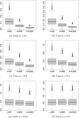
From this figure, it can be seen that:

• For small α, $n^{\alpha }\underset{x}{\sup }|F_n(x)-F_N(x)|$ rapidly decrease as the sample size n increases.

• As α increases, the decrease of $n^{\alpha }\underset{x}{\sup }|F_n(x)-F_N(x)|$ slows down as n increases.

• When α is 0.5, there is no change in the level of $n^{\alpha }\underset{x}{\sup }|F_n(x)-F_N(x)|$ even if n increases.

The simulation results are consistent with the theoretical conclusion that $n^{\alpha }\underset{x}{\sup }|F_n(x)-F_N(x)|$ ($\alpha <0.5$) converges to 0 when n (and N) goes to infinity. However, when α is 0.5, almost no convergence is observed.

4.2 Artificial population II

For another simulation, we use the finite population used by Sitter and Wu (2001), which is modified from that used by Francisco and Fuller (1991).

We generate the finite population from 10 stratum (subpopulations), whose proportions are 0.08, 0.08, 0.10, 0.10, 0.12, 0.12, 0.14, 0.10, 0.10, and 0.06, respectively. The values in each strata (subpopulation) are generated independently from 10 log-normal distributions whose mean and standard deviation of the distribution on the log-scale are $(1.5,0.3),(2.0,0.4),(2.1,0.4),(3.0,0.6),(2.5,0.5),(1.8,0.4),(1.6,0.3),(1.8,0.4),(3.0,0.6)$, and $(3.8,0.8)$, respectively.

The above data are stratified data, but in this simulation, to align our work with the theoretical results framework considered in this study, the simple random sampling without replacement method is utilized rather than using stratified sampling, wherein the strata structure is used in sampling.

Simulations are conducted in the same manner as for the artificial population I. As in Figure 2, each graph displays box plots with sample size 50 (population size 500), sample size 500 (population size 5, 000), and sample size 5, 000 (population size 50, 000), in order from left to right.

Fig. 2 (Artificial Population II) Box plots of the simulated values of $n^{\alpha }\underset{x}{\sup }|F_n(x)-F_N(x)|$ for various values of α. (Sample sizes of the box plots on each panel are 50, 500, and 5, 000, from left to right.)

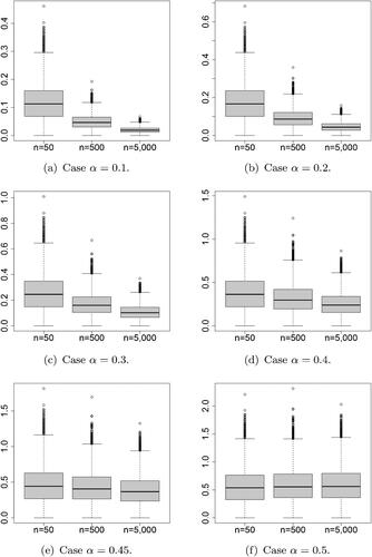
Overall, almost similar trends are observed in the simulation results of the artificial data II compared to the simulation of the artificial data I.

5 Concluding remarks

In this study, we evaluate the rate of uniform almost sure convergence of the empirical distribution function for simple random sampling without replacement from a finite population.

The results of the simulation studies are consistent with the theoretically derived results.

Acknowledgment

The author thanks two anonymous referees for their comments and suggestions which greatly helped to improve the article.

Disclosure statement

No potential conflict of interest was reported by the authors.

Additional information

Funding

This research was supported by a Grant-in-Aid for Scientific Research (Japan Society for the Promotion of Science) Grant Numbers 18H00837, 21K01429.

Appendix A

In this appendix, a direct proof of corollary 3.2 is given as a supplement. This proof involves almost the same lines as that of Fabian and Hannan (1985) for the I.I.D. case (See also Motoyama and Takahashi 2006).

Direct proof of Corollary 3.2. Define $${\Delta }_{N,n}=\underset{x}{\sup }|F_n(x)-F_N(x)|.$$

Let m be an integer, and consider the sets $$\left\{x:F_N(x)\in \left[0,\frac{1}{m}\right)\right\},\left\{x:F_N(x)\in \left[\frac{1}{m},\frac{2}{m}\right)\right\},\dots ,\left\{x:F_N(x)\in \left[\frac{m-1}{m},1\right]\right\}.$$

This is the sequence of intervals (A1) $$(a_0,a_1),[a_1,a_2),\dots ,[a_{m-1},a_m),\text{with}{a}_0=-\infty ,a_m=\infty .$$(A1)

As noted before, $\mathrm{I}(X_i\le x),i=1,\dots ,n$ is a simple random sample without replacement from $\mathrm{I}(x_i\le x),i=1,\dots ,N$, and $\mathrm{I}(X_i<x),i=1,\dots ,n$ is a simple random sample without replacement from $\mathrm{I}(x_i<x),i=1,\dots ,N$. Therefore, considering the finite population strong law of large numbers (Rosén 1965; Sen 1972), we obtain $$F_n(a_j)-F_N(a_j)\to 0,\hspace{1em}{F}_n(a_j-)-F_N(a_j-)\to 0$$for $j=1,\dots ,m-1$ on a set Ω_m of probability 1.

Let $x\in \mathbb{R}$, then x is in one of the intervals in (A1)(A1) $$(a_0,a_1),[a_1,a_2),\dots ,[a_{m-1},a_m),\text{with}{a}_0=-\infty ,a_m=\infty .$$(A1) , and thus $x\in [a_{i-1},a_i)\cap \mathbb{R}$ for some i and $$F_n(x)-F_N(x)\le F_n(a_i-)-F_N(a_{i-1})\le F_n(a_i-)-F_N(a_i-)+\frac{1}{m},$$and $$F_N(x)-F_n(x)\le F_N(a_i-)-F_n(a_{i-1})\le F_N(a_{i-1})-F_n(a_{i-1})+\frac{1}{m}.$$

Therefore, $${\Delta }_{N,n}\le {\max }_{i=1}^{m-1}\left[|F_n(a_i)-F_N(a_i)|+|F_n(a_i-)-F_N(a_i-)|\right]+\frac{2}{m}$$

and $\underset{N,n\to \infty }{\lim \sup }{\Delta }_{N,n}\le 2/m$ on Ω_m. Thus, $\underset{N,n\to \infty }{\lim \sup }{\Delta }_{N,n}=0$ on ${\Omega }_0={\cap }_{m=1}^{\infty }{\Omega }_m$ and $P({\Omega }_0)=1$. Hence, (4)(4) $$\underset{x}{\sup }|F_n(x)-F_N(x)|\to 0\hspace{1em}\mathrm{a}.\mathrm{s}.$$(4) is proven. □

References

- Bardenet, R., and O.-A. Maillard. 2015. Concentration inequalities for sampling without replacement. Bernoulli 21 (3):1361–85. doi: 10.3150/14-BEJ605.
- Boistard, H., H. P. Lopuhaä, and A. Ruiz-Gazen. 2017. Functional central limit theorems for single-stage sampling designs. The Annals of Statistics 45 (4):1728–58. doi: 10.1214/16-AOS1507.
- Bonnéry, D., F. J. Breidt, and F. Coquet. 2012. Uniform convergence of the empirical cumulative distribution function under informative selection from a finite population. Bernoulli 18 (4):1361–85. doi: 10.3150/11-BEJ369.
- Breidt, F., J. D. Jay, and Opsomer. 2008. Endogenous post-stratification in surveys: Classifying with a sample-fitted model. The Annals of Statistics 36 (1):403–27. doi: 10.1214/009053607000000703.
- Chatterjee, A. 2011. Asymptotic properties of sample quantiles from a finite population. Annals of the Institute of Statistical Mathematics 63 (1):157–79. doi: 10.1007/s10463-008-0210-4.
- Cheng, F. 2008. Extended Glivenko–Cantelli theorem in ARCH(p)-time series. Statistics & Probability Letters 78 (12):1434–9. doi: 10.1016/j.spl.2007.12.009.
- Cheng, F., J. Yan, and L. Yang. 2014. Extended Glivenko–Cantelli theorem in nonparametric regression. Communications in Statistics- Theory and Methods 43 (17):3720–5. doi: 10.1080/03610926.2012.700377.
- Conti, P. L. 2014. On the estimation of the distribution function of a finite population under high entropy sampling designs, with applications. Sankhya B 76 (2):234–59. doi: 10.1007/s13571-014-0083-x.
- Conti, P. L., and D. Marella. 2015. Inference for quantiles of a finite population: Asymptotic versus resampling results. Scandinavian Journal of Statistics 42 (2):545–61. doi: 10.1111/sjos.12122.
- Erdős, P., and A. Rényi. 1959. On the central limit theorem for samples from a finite population. Publications of the Mathematical Institute of the Hungarian Academy of Sciences 4:49–61.
- Fabian, V., and J. Hannan, 1985. Introduction to probability and mathematical statistics, In Probability and mathematical statistics: Probability and mathematical statistics, Wiley Series. New York: John Wiley & Sons, Inc.
- Francisco, C. A., and W. A. Fuller. 1991. Quantile estimation with a complex survey design. The Annals of Statistics 19 (1):454–69. doi: 10.1214/aos/1176347993.
- Hájek, J. 1960. Limiting distributions in simple random sampling from a finite population. Publications of the Mathematical Institute of the Hungarian Academy of Sciences 5:361–74.
- Han, Q., and J. A. Wellner. 2021. Complex sampling designs: Uniform limit theorems and applications. The Annals of Statistics 49 (1):459–85. doi: 10.1214/20-AOS1964.
- Horowitz, J. 1990. A uniform law of large numbers and empirical central limit theorem for limits of finite populations. Statistics & Probability Letters 10 (2):159–66. doi: 10.1016/0167-7152(90)90012-V.
- Loève, M. 1977. Probability theory. I. In Graduate texts in mathematics, 4th ed., 45. New York-Heidelberg: Springer-Verlag.
- Motoyama, H., and H. Takahashi, 2006. On estimators for finite population distributon function. (Yugen boshuudan niokeru bunpukansu no suitei). In Kakei deta no keizaibunseki to toukeiteki shuhou, ed. Yoshizoe, Y. Tokyo: Tokei Kenkyukai, 117–31 (in Japanese).
- Motoyama, H., and H. Takahashi. 2008. Smoothed versions of statistical functionals from a finite population. Journal of the Japan Statistical Society 38 (3):475–504. doi: 10.14490/jjss.38.475.
- Rényi, A. 1970. Probability theory. In North-Holland series in applied mathematics and mechanics, ed. László Vekerdi, vol. 10. Amsterdam: North-Holland Pub. Co.
- Rosén, B. 1965. Limit theorems for sampling from finite populations. Arkiv För Matematik 5 (5):383–424. doi: 10.1007/BF02591138.
- Rubin-Bleuer, S. 2003. On the convergence of sample empirical processes. Working Paper 03-3. Canada: Statistics Canada. Methodology Branch. https://publications.gc.ca/site/eng/9.840393/publication.html.
- Saegusa, T. 2019. Large sample theory for merged data from multiple sources. The Annals of Statistics 47 (3):1585–615. doi: 10.1214/18-AOS1727.
- Saegusa, T., and J. A. Wellner. 2013. Weighted likelihood estimation nder two-phase sampling. Annals of Statistics 41 (1):269–95. 24563559 doi: 10.1214/12-AOS1073.
- Sen, P. K. 1972. A Hájek-Rényi type inequality for generalized U-Statistics. Calcutta Statistical Association Bulletin 21 (3-4):171–80. doi: 10.1177/0008068319720306.
- Serfling, R. J. 1980. Approximation theorems of mathematical statistics. In Wiley series in probability and mathematical statistics. New York: John Wiley & Sons, Inc.
- Shao. 1994. L-statistics in complex survey problems. The Annals of Statistics 22 (2):946–67. doi: 10.1214/aos/1176325505.
- Shorack, G. R., and J. A. Wellner, 1986. Empirical processes with applications to statistics. In Wiley series in probability and mathematical statistics: Probability and mathematical statistics. New York: John Wiley & Sons, Inc.
- Sitter, R. R., and C. Wu. 2001. A note on Woodruff confidence intervals for quantiles. Statistics & Probability Letters 52 (4):207–15. doi: 10.1016/S0167-7152(00)00207-8.
- Van De Geer, S. A. 2000. Applications of empirical process theory. In Cambridge series in statistical and probabilistic mathematics. Vol. 6. Cambridge: Cambridge University Press.
- Van Der Vaart, A. W. 1998. Cambridge series in statistical and probabilistic mathematics. Vol. 3. Cambridge: Cambridge University Press. doi: 10.1017/CBO9780511802256.
- Van Der Vaart, A. W., and J. A. Wellner, 1996. Weak convergence and empirical processes. In Springer series in statistics, With applications to statistics. New York: Springer-Verlag. doi: 10.1007/978-1-4757-2545-2.
- Zhong, C. 2022. Extended Glivenko-Cantelli theorem and L1 strong consistency of innovation density estimator for time-varying semiparametric ARCH model. Journal of Nonparametric Statistics 35 (2):373–96. doi: 10.1080/10485252.2022.2152813.