Comparative study on excess distribution estimation in iid settings

Abstract.

This study considers excess distribution estimation in iid settings. There are two ways for the estimation; the fitting to the generalized Pareto distribution and the fully non parametric estimation. The fitting estimator is justified by the approximation proven in the extreme value theory; however, the accuracy depends on how extremely large the target is. The non parametric estimator does not need an approximation and has the advantage of wide applicability. This study conducts both theoretical and numerical comparative study on excess distribution estimation. Asymptotic convergence rates of two estimators are obtained, and the mean integrated squared errors are numerically surveyed by simulation study. An illustrative example of Abisko rainfall amount is presented.

Keywords:

• Excess distribution
• extreme value
• kernel type estimator
• mean squared error
• non parametric estimation

Mathematics Subject Classification (2010):

• 62G32
• 62G07
• 60G70

1. Introduction

Let $X_1,X_2,\cdots X_n$ be independent and identically distributed random variables with a continuous distribution function F. Suppose that n is sufficiently large. Here, we consider estimating the excess distribution (ED) given by $$\begin{array}{l}{F}_u(x):=P(X_1-u\le x|X_1>u)=\frac{F(x+u)-F(u)}{1-F(u)}.\end{array}$$

Shimokihara and Maesono (2018) studied asymptotic properties of a non parametric estimator. The non parametric estimator (NE) is the plug-in type of the kernel distribution estimator $$\begin{array}{l}{\hat{F}}_u(x):=\frac{\hat{F}(x+u)-\hat{F}(u)}{1-\hat{F}(u)},\end{array}$$ where $\hat{F}(x)$ is the kernel distribution estimator given by $$\begin{array}{l}\hat{F}(x)=\frac{1}{n}\sum _{i=1}^{n}W\left(\frac{x-X_i}{h}\right),\end{array}$$ where W is the cumulative distribution function of a symmetric density w. The bandwidth h is supposed to satisfy h→0.

Under some regularity conditions, the asymptotic mean squared error (MSE) of NE ${\hat{F}}_u(x)$ asymptotically equals $$\begin{array}{l}\frac{h^4}{4}{\left(\frac{1}{1-F(u)}\right)}^2{(f^{\prime }(x+u)-f^{\prime }(u)+F_u(x)f^{\prime }(u))}^2{(\int z^{2}w(z)\mathrm{d}z)}^2\\ +n^{-1}{F}_u(x)\frac{1-F(x+u)}{(1-F(u){)}^2}\end{array}$$

(see Theorem 1.1 in Shimokihara and Maesono 2018), where the integral range being $(-\mathrm{\infty },\mathrm{\infty })$ is omitted in this paper. Both x and u are implicitly assumed to be fixed in Shimokihara and Maesono (2018).

If we want to know the ED F_u(x) on a tail, the Pickands-Balkema-De Haan theorem in the extreme value theory is applicable. The theorem states that F_u(x) converges to the generalized Pareto distribution (GPD) H_{γ, c}(x) as $u\uparrow x^{\ast }:=sup(\mathrm{supp}(f))$, where $$\begin{array}{ll}{H}_{\gamma ,c}(x):=& H_{\gamma }\left(\frac{x}{c}\right)\mathrm{for}1+\gamma \frac{x}{c}>0,\\ H_{\gamma }(x):=& 1-\{\begin{array}{ll}(1+\gamma x{)}^{-1/\gamma }& \mathrm{for}1+\gamma x>0\mathrm{and}\gamma \in \mathbb{R}\setminus \{0\}\\ \exp (-x)& \mathrm{for}x\in \mathbb{R}\mathrm{and}\gamma =0.\end{array}\end{array}$$

Thus, parametrically fitting GPD to ED is justified, and $$\begin{array}{l}{H}_{{\hat{\mathit{\gamma }}}_u}(x):=H_{\hat{\gamma }}\left(\frac{x}{{\hat{c}}_u}\right)\mathrm{for}1+\hat{\gamma }\frac{x}{{\hat{c}}_u}>0\end{array}$$ provides good estimates for a sufficiently large u. We will call the parametric estimator PE.

In short, there are mainly two ways to estimate ED. NE ${\hat{F}}_u$ is supposed to be used for fixed, that is, not large u. On the other hand, the extreme value approach requires large u. Then, the following question arise: How large u should be for the extreme value approach ?. Preceding researches also states “How far can we extrapolate into the tails?” (Smith 1987, p.1194), “That is, an approximation to probabilities of extreme deviation is supposed, which is assumed to become increasingly accurate as one moves further from the range of the data, but whose concise accuracy is unknown” (in the abstract of Hall and Weissman 1997). Smith (1987) gave a response in terms of the convergence rate, which is a function of x (Remark of Theorem 8.1).

This study aims at clarifying how large the fitting estimator requires on u by comparing the two ways of ED estimation. Moriyama (2021) conducted a comparative study on the estimation of sample maximum distribution F^m between the extreme-value-based approach and non parametric approach and investigated both theoretical and numerical accuracy, depending on m. Estimators of extreme quantiles are numerically compared in Banfi, Cazzaniga, and De Michele (2022).

To the best of our knowledge, this is the first comparative study between the extreme-value-based approach and the non parametric approach in the distribution tail. This study assumes the tail of the underlying distribution to obtain the explicit form of asymptotic errors. Throughout this study, suppose that F belongs to either one of (i) the so-called Hall class of distributions (see Hall and Welsh 1984), (ii) the following Weibull class of distributions, and (iii) the bounded class of distributions (see, e.g., Stupfler 2016), which satisfy (i) $\mathrm{\exists }(\alpha ,\beta ,A,B)$ s.t. $\alpha >0,\beta \ge 2^{-1},A>0,B\ne 0$ and $$\begin{array}{l}{x}^{\alpha +\beta }\{1-F(x)-A{x}^{-\alpha }(1+B{x}^{-\beta })\}\to 0\mathrm{as}x\to \mathrm{\infty },\end{array}$$

(ii) $\mathrm{\exists }(\kappa ,C)$ s.t. $\kappa >0,C>0$ and $$\begin{array}{l}\exp (C{x}^{\kappa })\{1-F(x)-\exp (-C{x}^{\kappa })\}\to 0\mathrm{as}x\to \mathrm{\infty },\end{array}$$

(iii) $\mathrm{\exists }(x^{\ast },\mu ,\sigma ,D,E)$ s.t. $x^{\ast }\in \mathbb{R}$, $\mu <-2$, $\sigma \le -2^{-1}$, D > 0, E≠0 and $$\begin{array}{l}(x^{\ast }-x{)}^{\mu +\sigma }\{1-F(x)-(x^{\ast }-x{)}^{-\mu }(D+E(x^{\ast }-x{)}^{-\sigma })\}\to 0\mathrm{as}x\uparrow x^{\ast },\end{array}$$ respectively. Then, the limiting GPD is a Fréchet, Gumbel, and Weibull type under the supposition (see Beirlant et al. 2004), where $$\begin{array}{l}\gamma :=\{\begin{array}{ll}{\alpha }^{-1}& \mathrm{for}\mathrm{the}\mathrm{Hall}\mathrm{class}\\ 0& \mathrm{for}\mathrm{the}\mathrm{Weibull}\mathrm{class}\\ {\mu }^{-1}& \mathrm{for}\mathrm{the}\mathrm{bounded}\mathrm{class},\end{array}{c}_u:=\{\begin{array}{ll}\gamma u& \mathrm{for}\mathrm{the}\mathrm{Hall}\mathrm{class}\\ C^{-1}{\kappa }^{-1}{u}^{1-\kappa }& \mathrm{for}\mathrm{the}\mathrm{Weibull}\mathrm{class}\\ -\gamma (x^{\ast }-u)& \mathrm{for}\mathrm{the}\mathrm{bounded}\mathrm{class}.\end{array}\end{array}$$ under κ≤1.

Section 2 and 3 give the asymptotic properties of NE, the Kernel-type estimator, and PE, the fitting estimator to GPD, respectively, under the supposition $x:=x_n\to x_{\mathrm{\infty }}$ and $u:=u_n\to x^{\ast }$ as n→∞, where x_∞: = ∞ for the Hall class or the Weibull class and x_∞: = 0 for the bounded class. Results of the numerically comparative study are shown in Section 4, and the asymptotic convergence rates of the two estimators are provided in some cases. The proofs of theoretical results are in Appendix.

2. Kernel-type estimation

The following theorem on the MSE of NE is a consequence of Theorem 1.1 in Shimokihara and Maesono (2018), where all asymptotic notations in this article refer to n→∞.

Theorem 1.

Suppose F is continuously twice differentiable at x. If $\int z^{2}w(z)\mathrm{d}z<\mathrm{\infty }$ and $$\begin{array}{l}\{\begin{array}{ll}h{x}^{\kappa -1}\to 0& \mathrm{for}\mathrm{the}\mathrm{Weibull}\mathrm{class}\\ h(x^{\ast }-x{)}^{-1}\to 0\mathrm{and}h(x^{\ast }-x{)}^{-1}\to 0& \mathrm{for}\mathrm{the}\mathrm{bounded}\mathrm{class},\end{array}\end{array}$$ $$\begin{array}{l}{F}_u^{-2}(x)\mathbb{E}[(F_u(x)-{\hat{F}}_u(x){)}^2]\sim (U_n{h}^2\frac{{\xi }_n}{2}\int z^{2}w(z)\mathrm{d}z{)}^2+\frac{U_n(1-U_n)v_n}{n},\end{array}$$

where $$\begin{array}{ll}{U}_n:=& \{\begin{array}{ll}{(1+\frac{x}{u})}^{-\alpha }& \mathrm{for}\mathrm{the}\mathrm{Hall}\mathrm{class}\\ \exp (-C\{(x+u{)}^{\kappa }-u^{\kappa }\})& \mathrm{for}\mathrm{the}\mathrm{Weibull}\mathrm{class}\\ {(1-\frac{x}{x^{\ast }-u})}^{-\mu }& \mathrm{for}\mathrm{the}\mathrm{bounded}\mathrm{class},\end{array}\\ {\xi }_n:=& \{\begin{array}{ll}\alpha (\alpha +1)u^{-2}\{{(\frac{x}{u}+1)}^{-2}+1-2{(\frac{x}{u}+1)}^{\alpha }\}& \mathrm{for}\mathrm{the}\mathrm{Hall}\mathrm{class}\\ {\kappa }^2{C}^2\{(x+u{)}^{2\kappa -2}-u^{2\kappa -2}\}& \mathrm{for}\mathrm{the}\mathrm{Weibull}\mathrm{class}\\ \mu (\mu +1)(x^{\ast }-u{)}^{-2}& \\ \times \{{(1-\frac{x}{x^{\ast }-u})}^{-2}+1-2{(1-\frac{x}{x^{\ast }-u})}^{\mu }\}& \mathrm{for}\mathrm{the}\mathrm{bounded}\mathrm{class},\end{array}\\ v_n:=& \{\begin{array}{ll}{A}^{-1}{u}^{\alpha }& \mathrm{for}\mathrm{the}\mathrm{Hall}\mathrm{class}\\ \exp (C{u}^{\kappa })& \mathrm{for}\mathrm{the}\mathrm{Weibull}\mathrm{class}\\ D^{-1}(x^{\ast }-u{)}^{\mu }& \mathrm{for}\mathrm{the}\mathrm{bounded}\mathrm{class}.\end{array}\end{array}$$

The following Corollary 1 on the bandwidth minimizing the MSE follows from Theorem 1.

Corollary 1.

Suppose $|\int zW(z)w(z)\mathrm{d}z|<\mathrm{\infty }$ and $U_n^{-2}{\xi }_n^{-2}{\omega }_n{n}^{-1}\to 0$, where $$\begin{array}{l}{\omega }_n:=\{\begin{array}{ll}{A}^{-1}\alpha u^{\alpha -1}((1-U_n{)}^2+U_n^{1+\gamma })& \mathrm{for}\mathrm{the}\mathrm{Hall}\mathrm{class}\\ \kappa C\exp (C{u}^{\kappa })(u^{\kappa -1}(1-U_n{)}^2+(x+u{)}^{\kappa -1}{U}_n)& \mathrm{for}\mathrm{the}\mathrm{Weibull}\mathrm{class}\\ D^{-1}\mu (x^{\ast }-u{)}^{\mu -1}((1-U_n{)}^2+U_n^{1+\gamma })& \mathrm{for}\mathrm{the}\mathrm{bounded}\mathrm{class}.\end{array}\end{array}$$

Under the assumptions of Theorem 1, the optimal bandwidth in the sense of the MSE is $$\begin{array}{l}h={\left(2U_n^{-2}{\xi }_n^{-2}{\omega }_n{n}^{-1}\frac{\int zW(z)w(z)\mathrm{d}z}{{(\int z^{2}w(z)\mathrm{d}z)}^2}\right)}^{1/3}.\end{array}$$

$F_u(x)-{\hat{F}}_u(x)$ with the optimal bandwidth is asymptotically non degenerate normal with the asymptotic mean $$\begin{array}{l}{\nu }_0{n}^{-2/3}{U}_n^{-1/3}{\xi }_n^{-1/3}{\omega }_n^{2/3},\end{array}$$

where ${\nu }_0:={(2\int z^{2}w(z)\mathrm{d}z)}^{-1/3}{(\int zW(z)w(z)\mathrm{d}z)}^{2/3}$.

The following Corollary 2 states the special case U_n = O(1) of Corollary 1.

Corollary 2.

Suppose ${}^{\mathrm{\exists }}\delta >0$ s.t. U_n→δ. Under the assumptions of Corollary 1, the asymptotically optimal bandwidth in the sense of the MSE is $$\begin{array}{ll}h=& {(2{\delta }^{-2}\{(1-\delta {)}^2+{\delta }^{1+\gamma }\}{n}^{-1}\frac{\int zW(z)w(z)\mathrm{d}z}{{(\int z^{2}w(z)\mathrm{d}z)}^2})}^{1/3}\\ \times & \{\begin{array}{ll}{A}^{-1/3}{\alpha }^{1/3}(\alpha +1{)}^{-2/3}{u}^{(\alpha +3)/3}({\delta }^{2\gamma }+1-2\delta {)}^{-2/3}& \mathrm{for}\mathrm{the}\mathrm{Hall}\mathrm{class}\\ {\kappa }^{-1}{C}^{-1/3}\exp (C{u}^{\kappa }/3)(-\ln \delta {)}^{-2/3}{u}^{1-(\kappa /3)}& \mathrm{for}\mathrm{the}\mathrm{Weibull}\mathrm{class}\\ D^{-1/3}{\mu }^{1/3}(\mu +1{)}^{-2/3}(x^{\ast }-u{)}^{(\mu +3)/3}({\delta }^{2\gamma }+1-2\delta {)}^{-2/3}& \mathrm{for}\mathrm{the}\mathrm{bounded}\mathrm{class}.\end{array}\end{array}$$

${\hat{F}}_u(x)$ with the optimal bandwidth has the asymptotic bias $$\begin{array}{ll}& {\nu }_0{\delta }^{-1/3}{((1-\delta {)}^2+{\delta }^{1+\gamma })}^{2/3}{n}^{-2/3}\\ \times & \{\begin{array}{ll}{A}^{-2/3}{\alpha }^{1/3}(\alpha +1{)}^{-1/3}{u}^{2\alpha /3}({\delta }^{2\gamma }+1-2\delta {)}^{-1/3}& \mathrm{for}\mathrm{the}\mathrm{Hall}\mathrm{class}\\ C^{1/3}(-\ln \delta {)}^{-1/3}\exp (2C{u}^{\kappa }/3)u^{\kappa /3}& \mathrm{for}\mathrm{the}\mathrm{Weibull}\mathrm{class}\\ D^{-2/3}{\mu }^{1/3}(\mu +1{)}^{-1/3}(x^{\ast }-u{)}^{2\mu /3}({\delta }^{2\gamma }+1-2\delta {)}^{-1/3}& \mathrm{for}\mathrm{the}\mathrm{bounded}\mathrm{class}.\end{array}\end{array}$$

The twice differentiability required in Theorem 1 is the usual regularity condition in smooth distribution estimation or density estimation (see, e.g., Wand and Jones 1995).

Remark 1.

x satisfying $\underset{n\to \mathrm{\infty }}{lim}h(x^{\ast }-x{)}^{-1}>0$ is called a boundary point in the naive kernel distribution estimation and the convergence rate of ${\hat{F}}_u(x)$ changes (see the proof of Theorem 1). Theorem 1 requires that μ is an integer or $\mu <-2$.

3. Fitting estimator to GPD

We employ the maximum likelihood estimation (MLE) based on the peak-over-threthold (POT) for fitting to the GPD, which was developed by Pickands (1975). Let t: = t_n be the threshold of the POT and N be the number of $X_1,X_2,\cdots X_n$ exceeding t. Let Y_j be the jth number of $X_1,X_2,\cdots X_n$ exceeding t $(j=1,\cdots ,N)$. It holds that $(N/N^{\ast })\stackrel{p}{\to }1$, where $N^{\ast }:=n(1-F(t))$. $\stackrel{p}{\to }$ means the probability convergence. Set ${\mathit{\gamma }}_t:=({\gamma }_t,c_t{)}^{\mathsf{T}}$ and $$\begin{array}{l}{\hat{\mathit{\gamma }}}_t:=\underset{{\mathit{\gamma }}_t}{\arg \max }\sum _{j=1}^N\ln h_{{\mathit{\gamma }}_t}(Y_j),\end{array}$$ where h_𝜸 is the density function of H_𝜸. Then, t needs to satisfy the following assumption.

Assumption 1.

Either (i)$(U_n\vee T_n)\to 0$ or (ii)${}^{\mathrm{\exists }}\delta >0$ s.t. both U_n→δ and T_n→δ holds, where $$\begin{array}{l}{T}_n:=\{\begin{array}{ll}{(1+\frac{x}{t})}^{-\alpha }& \mathrm{for}\mathrm{the}\mathrm{Hall}\mathrm{class}\\ \exp (-C\kappa t^{\kappa -1}x)& \mathrm{for}\mathrm{the}\mathrm{Weibull}\mathrm{class}\\ {(1-\frac{x}{x^{\ast }-t})}^{-\mu }& \mathrm{for}\mathrm{the}\mathrm{bounded}\mathrm{class}.\end{array}\end{array}$$

PE, the fitting estimator, fundamentally depends on the approximation based on the Pickands-Balkema-De Haan theorem shown in the following Proposition 1, whose convergence is ensured by Assumption 1.

Proposition 1.

Under Assumption 1 $$\begin{array}{l}{\tau }_n:=F_u(x)-H_{{\mathit{\gamma }}_t}(x)\to 0.\end{array}$$

Remark 2.

The condition (i) in Assumption 1 $$\begin{array}{l}{U}_n\to 0⟺\{\begin{array}{ll}u=o(x)& \mathrm{for}\mathrm{the}\mathrm{Hall}\mathrm{class}\\ u=o(x^{(1-\kappa {)}^{-1}})\mathrm{or}\kappa \ge 1& \mathrm{for}\mathrm{the}\mathrm{Weibull}\mathrm{class}\\ (x^{\ast }-u{)}^{-1}=o(x^{-1})& \mathrm{for}\mathrm{the}\mathrm{bounded}\mathrm{class}\end{array}\end{array}$$ restricts the threshold t to being asymptotically same as u in the following sense $$\begin{array}{l}\{\begin{array}{ll}t=o(x)& \mathrm{for}\mathrm{the}\mathrm{Hall}\mathrm{class}\\ t=o(x^{(1-\kappa {)}^{-1}})\mathrm{or}\kappa \ge 1& \mathrm{for}\mathrm{the}\mathrm{Weibull}\mathrm{class}\\ (x^{\ast }-t{)}^{-1}=o(x^{-1})& \mathrm{for}\mathrm{the}\mathrm{bounded}\mathrm{class}.\end{array}\end{array}$$ $$\begin{array}{l}{U}_n\to \delta ⟺\{\begin{array}{ll}u=({\delta }^{-\gamma }-1{)}^{-1}x+o(1)& \mathrm{for}\mathrm{the}\mathrm{Hall}\mathrm{class}\\ u=[-(Cx{)}^{-1}\ln \delta {]}^{(\kappa -1{)}^{-1}}+o(x^{(1-\kappa {)}^{-1}})& \mathrm{for}\mathrm{the}\mathrm{Weibull}\mathrm{class}\\ u=x^{\ast }+({\delta }^{-\gamma }-1{)}^{-1}x+o(x)& \mathrm{for}\mathrm{the}\mathrm{bounded}\mathrm{class},\end{array}\end{array}$$ where the Weibull class additionally needs both x = o(u) and κ < 1. (ii) being true requires t to be asymptotically same as u in a similar sense, as (i).

MLE is asymptotically efficient; however, various approaches are proposed and compared (Zhang 2007; Del Castillo and Serra 2015; Kang and Song 2017). Smith (1987) gave the conditions that show the following scaled version of the MLE $$\begin{array}{l}{\hat{\mathit{\gamma }}}_t^{\ast }=\left(\begin{array}{c}1\\ & c_t^{-1}\end{array}\right){\hat{\mathit{\gamma }}}_t\end{array}$$ is asymptotically normal with a non trivial bias and $\sqrt{N^{\ast }}$-consistent under the following Assumption 2.

Assumption 2.

${}^{\mathrm{\exists }}\lambda \in \mathbb{R}$ s.t. λ_n→λ, where $$\begin{array}{l}{\lambda }_n:=\sqrt{n}\times \{\begin{array}{ll}{A}^{1/2}{t}^{-\alpha /2}& \mathrm{for}\mathrm{the}\mathrm{Hall}\mathrm{class}\\ -t^2\exp (-C{t}^{\kappa })& \mathrm{for}\mathrm{the}\mathrm{Weibull}\mathrm{class}\\ D^{1/2}(x^{\ast }-t{)}^{-\mu /2}& \mathrm{for}\mathrm{the}\mathrm{bounded}\mathrm{class}\end{array}\end{array}$$

We have the following proposition on the accuracy of PE, which is a consequence of Smith (1987).

Proposition 2.

Under Assumptions 1–2 $$\begin{array}{l}\mathbb{E}[(F_u(x)-H_{{\hat{\mathit{\gamma }}}_t}(x){)}^2]\sim ({\tau }_n+{N^{\ast }}^{-1/2}{\lambda }_n{\mathit{\eta }}_n^{\mathsf{T}}{\mathrm{\Sigma }}_0^{-1}\mathit{\mu }{)}^2+{N^{\ast }}^{-1}({\mathit{\eta }}_n^{\mathsf{T}}{\mathrm{\Sigma }}_0^{-1}{\mathit{\eta }}_n),\end{array}$$

where 𝛍 and the Fisher information matrix Σ₀ are given in Smith (1987), and $$\begin{array}{l}{\mathit{\eta }}_n:={(T_n(-T_n^{\gamma }+1+\gamma \ln T_n),\frac{1-T_n^{-\gamma }}{\gamma }{T}_n^{1+\gamma })}^{\mathrm{\top }}.\end{array}$$

The following corollary on the convergence rate of PE immediately follows from Proposition 2.

Corollary 3.

Under the assumptions of Proposition 2, $(F_u(x)-H_{{\hat{\mathit{\gamma }}}_t}(x))$ converges with the rate larger of τ_n and ${N^{\ast }}^{-1/2}{\mathit{\eta }}_n^{\mathrm{\top }}\mathbf{1}$.

4. Comparative study

Suppose $t=u^{\ast }$ and ${}^{\mathrm{\exists }}\delta >0$ s.t. U_n≡δ throughout in this section, where $$\begin{array}{l}{u}^{\ast }:=\{\begin{array}{ll}u& \text{for the Hall class or the Weibull class}\\ (x^{\ast }-u{)}^{-1}& \text{for the bounded class}.\end{array}\end{array}$$

Set the threshold $u^{\ast }=n^{1/8}$, $u^{\ast }=n^{1/4}$, $u^{\ast }=n^{1/2}$, or $u^{\ast }=n^{3/4}$. Since ${\tau }_n\sim T_n-U_n+O((u^{\ast }{)}^{-\beta })$ for the Hall class, the MSE of PE converges with the rate $n^{-1}(u^{\ast }{)}^{\alpha }+(u^{\ast }{)}^{-2\beta }$. The MSE for the bounded class is of order $n^{-1}(u^{\ast }{)}^{-\mu }+(u^{\ast }{)}^{2\sigma }$. The minimum of the MSE of NE is of order $n^{-1}(u^{\ast }{)}^{\alpha }$ or $n^{-1}(u^{\ast }{)}^{-\mu }$ for the Hall class or the bounded class if the minimizing bandwidth converges, that is, $n^{-1}(u^{\ast }{)}^{\alpha +3}\to 0$ or $n^{-1}(u^{\ast }{)}^{-\mu +3}\to 0$, respectively. For the Weibull class, the MSE of PE does not converge to zero when u is of the polynomial order of n, and the MSE of NE tends to infinity. If $u=(\ln n{)}^{1/\kappa }$, the MSE of PE converges order slower than any polynomial, the asymptotic variance n^C−1 converges. The order of the MSE of NE $n^{(4/3)(C-1)}(\ln n{)}^{2/3}$ in the setting.

To sum up, when F belongs to the Hall class or the bounded class, NE converges with the same or faster rate than PE if the optimal bandwidth converges. Specifically, whether PE should be used depends on $n^{-1}(u^{\ast }{)}^{(1/|\gamma |)+3}$ converges or not. For the Weibull class, the two estimators are not consistent if the threshold u is a polynomial order of n.

Next, the underlying distributions F were supposed to be Burr distributions defined as $1-F(x)=(1+x^c{)}^{\ell }$, where α = cℓ and β = c, Weibull distributions, and inverse Burr distributions defined as $1-F(x)=(1+(-x{)}^{\ell }{)}^{c}x<0$, where μ = cℓ and $\sigma =1/c$. The parameters of the underlying distributions and the convergence rates of MSE without terms slower than any polynomial are summarized in Table 1, where the tail index γ is α⁻¹, zero and μ⁻¹, respectively. The hyphen means the distribution breaks the assumption of this study of the estimator. The Weibull class with γ = 0 breaks both the assumptions of PE and NE. For $u^{\ast }=n^{1/8}$ (small relative to n) and γ far from zero, the convergence rate of MSE of NE is fast and especially close to n⁻¹ for α or μ being close to zero while that of PE is quite slow. The relation to the convergence rate of PE is complicated, unlike that of NE. As u^* gets relatively large, the convergence rate of PE becomes faster, but the requirement becomes restrictive in general. Particularly, the assumption is broken for γ being close to zero. NE loses its consistency completely if $n^{1/2}(u^{\ast }{)}^{-1}$ converges to some constant, including zero.

Table 1. The polynomial convergence rates of the MSE of the estimators and the lengths.

Burr			$u^{\ast }=n^{1/8}$		$u^{\ast }=n^{1/4}$		$u^{\ast }=n^{1/2}$		$u^{\ast }=n^{3/4}$
c, ℓ	α	β	PE	NE	PE	NE	PE	NE	PE	NE
1/2,1/2	1/4	1/2	−1/8	−31/32	−1/4	−15/16	−1/2	–	−13/16	–
1,1/2	1/2	1	−1/4	−15/16	−1/2	−7/8	−3/4	–	−5/8	–
3,1/2	3/2	3	−3/4	−13/16	−5/8	–	−1/4	–	–	–
1/2,1	1/2	1/2	−1/8	−15/16	−1/4	−7/8	−1/2	–	−5/8	–
1,1	1	1	−1/4	−7/8	−1/2	–	−1/2	–	−1/4	–
3,1	3	3	−5/8	−5/8	−1/4	–	–	–	–	–
1/2,3	3/2	1/2	−1/8	−13/16	−1/4	–	−1/4	–	–	–
1,3	3	1	−1/4	−5/8	−1/4	–	–	–	–	–
3,3	9	3	–	–	–	–	–	–	–	–
Weibull			$u^{\ast }=n^{1/8}$		$u^{\ast }=n^{1/4}$		$u^{\ast }=n^{1/2}$		$u^{\ast }=n^{3/4}$
κ	γ	ρ	PE	NE	PE	NE	PE	NE	PE	NE
1/2	0	0	–	–	–	–	–	–	–	–
1	0	0	–	–	–	–	–	–	–	–
3	0	0	–	–	–	–	–	–	–	–
10	0	0	–	–	–	–	–	–	–	–
inv. Burr			$u^{\ast }=n^{1/8}$		$u^{\ast }=n^{1/4}$		$u^{\ast }=n^{1/2}$		$u^{\ast }=n^{3/4}$
c, ℓ	μ	σ	PE	NE	PE	NE	PE	NE	PE	NE
3, 2	−6	−2	−1/4	–	–	–	–	–	–	–
1, 2	−2	−2	−1/2	−3/4	−1/2	–	–	–	–	–
1/2, 2	−1	−2	−1/2	−7/8	−3/4	–	−1/2	–	−1/4	–
3, 1	−3	−1	−1/4	−5/8	−1/4	–	–	–	–	–
1, 1	−1	−1	−1/4	−7/8	−1/2	–	−1/2	–	−1/4	–
1/2, 1	−1/2	−1	−1/4	−15/16	−1/2	−7/8	−3/4	–	−5/8	–
3, 1/3	−1	−1/3	−1/12	−7/8	−1/6	–	−1/3	–	−1/4	–
1, 1/3	−1/3	−1/3	−1/12	−23/24	−1/6	−11/12	−1/3	–	−1/2	–
1/2, 1/3	−1/6	−1/3	−1/12	−47/48	−1/6	−23/24	−1/3	–	−1/2	–

By simulating the following, the mean integrated squared error (MISE) of PE $$\begin{array}{l}{L}_u^{-1}{\int }_{Q_u(0.1)}^{Q_u(0.9)}{(H_{{\hat{\mathit{\gamma }}}_t}(x)-F_u(x))}^2\mathrm{d}x.\end{array}$$ and that of NE ${\hat{F}}_u$, we studied the numerical accuracy in finite-sample cases. $L_u:=Q_u(0.9)-Q_u(0.1)$, and Q_u(q) denotes the qth quantile of the ED. We suppose $Q_u(q)(0.1\le q\le 0.9)$, which is intended that U_n = O(1), that is, $F_u(x)\sim \exp (-U_n)=O(1)$. This numerical study employs $\hat{h}:=n^{-1/3}{u}^{1+({\hat{\gamma }}^{-1}/3)}$ as the bandwidth estimator following the result in Corollary 2, where $\hat{\gamma }$ is the MLE. The kernel functions were the Epanechnikov for the inverse Burr distributions and the Gaussian for the other distributions. We simulated the MISE values 10,000 times, where Tables 2–5 show the mean values and their standard deviation (sd), where the hyphens mean $1-F(u^{\ast })$ numerically equals zero, and so we cannot derive the MISE value. The sample sizes were (n =) 2⁸ or 2¹². u^* is n^1∕8, n^1∕4 or n^1∕2.

Table 2. Scaled MISE values (×100) and sd values (×100) for the estimators.

Burr	n = 2^8				n = 2^12
	PE	sd	NE	sd	PE	sd	NE	sd
c, ℓ	u = 2				$u=2^{3/2}$
1/2,1/2	0.085	0.161	0.066	0.074	0.417	0.565	0.004	0.005
1,1/2	0.056	0.073	0.079	0.080	0.043	0.709	0.006	0.006
3,1/2	0.139	0.182	0.152	0.153	0.013	0.017	0.018	0.019
1/2,1	0.077	0.096	0.112	0.113	0.023	0.381	0.008	0.008
1,1	0.129	0.155	0.167	0.164	0.010	0.012	0.014	0.014
3,1	0.515	0.727	0.341	0.397	0.072	0.092	0.080	0.084
1/2,3	0.718	0.975	0.760	0.800	0.049	0.062	0.070	0.069
1,3	2.078	2.786	1.268	1.397	0.184	0.408	0.197	0.207
3,3	8.467	5.770	4.048	3.513	–	–	–	–
c, ℓ	u = 2^2				u = 2^3
1/2,1/2	0.061	0.095	0.079	0.082	0.141	0.221	0.043	0.020
1,1/2	0.073	0.098	0.098	0.098	0.016	0.226	0.010	0.010
3,1/2	0.389	0.492	0.391	0.398	0.063	0.083	0.076	0.077
1/2,1	0.098	0.122	0.123	0.114	0.008	0.010	0.012	0.012
1,1	0.226	0.278	0.275	0.266	0.021	0.026	0.030	0.030
3,1	5.031	5.550	3.310	4.391	2.639	3.517	1.925	2.310
1/2,3	1.793	2.668	1.449	1.529	0.160	0.201	0.197	0.198
1,3	6.413	5.378	6.785	6.686	3.832	4.364	3.374	4.222
3,3	10.452	5.223	12.662	1.048	–	–	–	–
c, ℓ	u = 2^4				u = 2^6
1/2,1/2	0.068	0.087	0.201	0.157	0.135	0.156	0.326	0.055
1,1/2	0.137	0.175	0.524	0.245	0.019	0.051	1.125	0.167
3,1/2	4.634	5.841	4.511	6.116	2.534	3.493	2.448	2.695
1/2,1	0.172	0.243	0.683	0.279	0.021	0.048	1.281	0.173
1,1	0.907	1.152	1.161	0.946	0.021	0.048	1.281	0.173
3,1	8.952	3.599	32.555	20.262	10.875	2.193	39.079	18.143
1/2,3	7.158	7.335	9.564	11.507	3.685	4.930	3.861	5.144
1,3	9.905	3.787	39.100	18.296	10.896	2.682	41.768	16.961
3,3	15.334	2.374	47.800	0.000	–	–	–	–

Table 3. Scaled MISE values (×100) and sd values (×100) for the estimators.

inv. Burr	n = 2^8				n = 2^12
	PE	sd	NE	sd	PE	sd	NE	sd
c, ℓ	u = 2^2				u = 2^3
3, 2	26.100	0.000	2.464	0.321	24.700	0.000	1.891	0.087
1, 2	7.580	0.000	0.533	0.139	6.590	0.000	0.307	0.032
1/2, 2	0.159	0.179	1.405	0.275	0.013	0.018	0.453	0.061
3,1	10.400	0.000	0.719	0.091	9.390	0.000	0.477	0.055
1,1	0.744	0.075	0.510	0.165	0.381	0.004	0.152	0.021
1/2,1	0.412	0.481	3.696	0.887	0.071	0.100	1.695	0.184
3,1/3	0.777	1.205	0.504	0.332	0.037	0.054	0.203	0.077
1,1/3	0.965	0.635	2.396	1.169	0.186	0.254	1.237	0.291
1/2,1/3	15.160	2.634	8.225	0.749	8.872	6.600	3.487	1.728
c, ℓ	u = 2^4				u = 2^6
3, 2	23.500	0.000	0.717	0.002	21.500	0.000	0.952	0.007
1, 2	5.881	0.003	3.034	0.196	5.010	0.000	4.573	0.043
1/2, 2	0.448	0.363	11.084	0.991	0.069	0.102	15.179	0.631
3,1	8.573	0.005	2.251	0.068	7.280	0.000	3.688	0.041
1,1	0.290	0.104	6.982	0.377	0.063	0.009	9.445	0.103
1/2,1	4.097	4.593	15.750	0.782	2.168	2.461	19.648	3.885
3,1/3	0.893	1.252	7.575	0.925	0.099	0.144	11.678	0.753
1,1/3	2.708	3.437	14.700	1.138	2.793	3.459	18.732	3.054
1/2,1/3	17.040	8.314	25.870	0.389	10.516	7.941	26.731	0.876
c, ℓ	u = 2^6				u = 2^9
3, 2	19.900	0.000	7.125	0.016	17.900	0.000	9.620	0.000
1, 2	4.574	0.010	16.540	0.052	4.240	0.000	19.100	0.006
1/2, 2	4.367	4.818	32.050	1.002	1.525	2.540	34.679	0.212
3,1	6.370	0.012	14.760	0.052	5.250	0.001	17.805	0.022
1,1	0.368	0.651	26.410	0.074	0.053	0.128	29.613	0.050
1/2,1	17.667	9.352	37.460	0.052	28.320	6.218	39.951	0.272
3,1/3	10.731	10.665	29.110	0.152	2.337	4.374	33.221	0.165
1,1/3	20.466	6.344	36.810	0.120	28.531	6.543	39.767	0.199
1/2,1/3	16.780	19.468	42.390	0.032	30.408	12.21	44.101	0.018

Table 4. Scaled MISE values (×100) and sd values (×100) for the estimators.

Weibull	n = 2^8				n = 2^12
	PE	sd	NE	sd	PE	sd	NE	sd
κ, C	u = 2^2				u = 2^3
1/2, 1	0.229	0.658	0.246	0.257	0.020	0.021	0.021	0.021
1, 1	0.425	0.603	0.301	0.348	–	–	–	–
3, 1	–	–	–	–	–	–	–	–
10, 1	–	–	–	–	–	–	–	–
κ, C	u = 2^4				u = 2^6
1/2, 1	0.402	0.538	0.414	0.453	0.051	0.066	0.063	0.065
1, 1	4.078	4.156	2.208	2.883	–	–	–	–
3, 1	–	–	–	–	–	–	–	–
10, 1	–	–	–	–	–	–	–	–
κ, C	u = 2^5				u = 2^9
1/2, 1	4.272	4.354	3.590	4.205	6.682	5.021	11.531	9.561
1, 1	4.078	4.156	36.876	17.292	–	–	–	–
3, 1	–	–	–	–	–	–	–	–
10, 1	–	–	–	–	–	–	–	–

Table 5. Scaled MISE values (×100) and sd values (×100) for the estimators.

Weibull	n = 2^8				n = 2^12
	PE	sd	NE	sd	PE	sd	NE	sd
κ, C	$u=(\ln n{)}^{1/\kappa }$
1/2, 1	8.013	5.481	13.924	10.731	7.882	5.686	20.619	16.486
1, 1	7.673	5.664	7.162	6.460	7.255	5.602	10.879	8.304
3, 1	7.799	6.144	1.710	1.207	7.626	5.940	1.308	1.785
10, 1	7.949	6.228	22.972	0.617	7.705	6.095	9.079	0.482
κ, C	$u=(\ln n{)}^{1/\kappa }$
1/2, 1/2	5.690	6.383	4.910	6.881	3.603	4.349	2.729	3.361
1, 1/2	6.902	5.369	5.265	3.227	5.112	2.103	4.897	1.692
3, 1/2	25.110	1.504	27.714	1.080	25.471	0.470	27.283	0.441
10, 1/2	41.092	0.084	43.492	0.077	42.322	0.060	44.371	0.045
κ, C	$u=(\ln n{)}^{1/\kappa }$
1/2, 1/5	7.846	4.927	6.414	3.756	6.702	1.960	6.399	1.771
1, 1/5	20.343	2.531	20.126	2.388	20.116	0.834	20.085	0.923
3, 1/5	40.452	0.242	43.002	0.310	41.155	0.099	43.483	0.112
10, 1/5	43.112	0.032	43.800	0.000	44.100	0.005	44.600	0.000

Table 2 shows the simulated results on the MISE values for the Burr cases. On the whole, NE surpasses PE for relatively small u^* for example, $u^{\ast }=n^{1/8}$ and conversely, PE is better for $u^{\ast }=n^{1/2}$. The MISE values of NE are especially large for both α and u^* being large. For u^* being around n^1∕4 they are comparable. For $u^{\ast }\gtrsim n^{1/2}$ (e.g. $u^{\ast }=n$) it is thought that PE far outperforms NE and NE is of no use.

Table 3 shows the MISE values for the inverse Burr cases. NE gets inaccurate as u^* becomes large relatively to n; however, the performances of PE and NE heavily depend on not only the size of u^* but also the tail index γ. This numerical property is slightly different from that of the Burr cases. For $\gamma =-1/6$ (i.e. $c=3,\ell =2$) which is closest to zero in this study, NE is always more accurate than PE. Conversely, even though u^* is small, PE outperforms NE for some cases γ being around −1 to −3.

Table 4 shows the MISE values for the Weibull cases. Due to the light-tailness, 1−F(u) numerically equals zero in many cases. The remaining cases shows PE and NE are comparable, while PE is more numerically stable. In order to continue the comparative study on the Weibull cases, we chose relatively smaller (ln⁡n)^1∕κ as the threshold u^*. Table 5 shows the simulated results on the MISE values. In this setting, $1-F(u^{\ast })\sim \exp (C)n^{-1}$. We chose 1, 1∕2, and 1∕5 as the parameter C, where the tail gets lighter as C becomes small. For κ = 3 and C = 1, NE is quite accurate, but PE is much better than NE for $\kappa =1/2$ and C = 1 and κ = 10 and C = 1. For the other cases, they are comparable, and so we cannot conclude which one is better for the Weibull cases. For the light-tailed distribution, ED is considered to be quite sensitive to the distribution parameters. This study concludes PE and NE are comparable for the Weibull cases; however, more detailed numerical study is an important future work.

5. Real data study

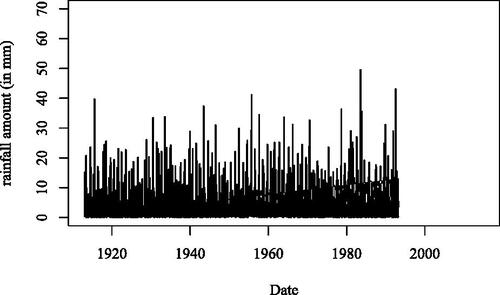
This section considers a real-data study. The data is on Abisko rainfall provided by Abisko Scientific Research Station. It is available in mev package in the R software environment. The data includes the rainfall amount (in mm) and the dates from 1/1/1913 to 1/1/2015, which is given in Figure 1. The time series trend was analyzed by the annual maximums and found to be not statistically significant (Rudvik 2012). Kiriliouk et al. (2019) applied the GPD fitting with the threshold u = 12 and showed $\hat{\gamma }\fallingdotseq 0$.

Figure 1. Abisko rainfall amount (in mm) from 1/1/1913 to 1/1/2015.

Extreme rainfall causes a landslide, and so a probability estimation is required. Figure 2 shows the estimated ED functions of Abisko rainfall amount (in mm) by the non parametric approach (solid line) and by fitting to the GPD (dashed line). The difference between the two approaches is found to be small. Figure 3 is the magnified Figure 2 at the area [7, 14] and shows the little difference; however, the difference is less than around 4%. In this area, the non parametric approach tends to return larger values, which means a pessimistic prospect.

Figure 2. The estimated ED functions of Abisko rainfall amount (in mm) from 1/1/1913 to 1/1/2015 data by the non parametric approach (solid line) and by the fitting to the GPD (dashed line).

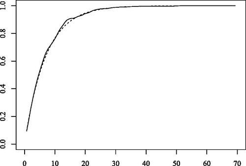
Figure 3. The estimated ED functions in [7, 14] of the Abisko rainfall amount (in mm) by the nonparametric approach (solid line) and by the fitting to the GPD (dashed line).

6. Conclusion and discussion

This study investigates the two estimators, PE and NE, of the ED above the threshold u and compares their accuracy. Asymptotic MSE of the estimators are derived and numerical study is conducted. Theoretical investigation reveals the followings. The threshold as the hyperparameter of PE denoted by t needs to be asymptotically same as u (see Assumption 1). The MSE of NE and the minimizing hyperparameter (bandwidth h) are presented. For the Weibull class, the two estimators of the ED of a polynomial order are not consistent. For the Hall class or bounded class, the accuracy of the two estimators depends on both u and the parameter γ. As u becomes larger relative to n, the two estimators tend to lose consistency. When u is small relative to n, NE is theoretically superior to PE in general. When u is large relative to n, PE excels NE. If γ > 0, the heavier the tail is, the better NE works. If γ < 0, NE outperforms PE, especially for γ being close to zero. Simulation study mostly demonstrates the asymptotic supremacy of each of the estimators. In the real data study, the difference between the two estimators are surveyed. It is found that the difference is slight, but the non parametric approach returns an estimated probability slightly larger.

The obtained result of the comparative study is different from that of distribution estimation of sample maximum. By comparing the fitting estimator to the generalized extreme value distribution and the non parametric kernel type estimator, Moriyama (2021) demonstrated that the non parametric estimator is good in the case γ≒0, where the fitting estimator loses consistency. That means the performance of non parametric estimation in extreme value analysis depends on at least the target being related to the generalized Pareto distribution or the generalized extreme value distribution. This fact suggests the properties of other non parametric estimators in extreme value analysis. In order to improve the accuracy of extreme value inference, we need to continue to clarify the properties of the non parametric estimators.

Data availability

The dataset analyzed during the current study is available in the mev package in the R software environment.

Acknowledgments

The author appreciates the editor’s and referees’ valuable comments that helped us improve this manuscript.

Disclosure statement

The author declares that there are no conflicts of interest.

Additional information

Funding

This work was supported by JSPS KAKENHI Grant Number JP23K16850.

Appendix

Proof of Proposition 1.

For the Hall class, it follows from $\gamma ={\alpha }^{-1}$ and c_t = γt that $$\begin{array}{l}{H}_{{\mathit{\gamma }}_t}(x)=1-{(1+\frac{x}{t})}^{-\alpha }=1-T_n.\end{array}$$

Since $$\begin{array}{l}{F}_u(x)=1-{(1+\frac{x}{u})}^{-\alpha }+O\left(u^{-\beta }{(1+\frac{x}{u})}^{-\alpha }\right),\end{array}$$ we see ${\tau }_n:=F_u(x)-H_{{\mathit{\gamma }}_t}(x)\to 0$ if either (i) $(U_n\vee T_n)\to 0$ or (ii) ${}^{\mathrm{\exists }}\delta >0$ s.t. U_n→δ and T_n→δ holds, which means $t=u=O(x)$. Then, $$\begin{array}{l}{\tau }_n\sim T_n-U_n+O(u^{-\beta }).\end{array}$$

For the Weibull class, it follows from γ = 0 and $c_t={\kappa }^{-1}{t}^{1-\kappa }$ that $$\begin{array}{l}{H}_{{\mathit{\gamma }}_t}(x)=1-\exp (-C\kappa t^{\kappa -1}x)=1-T_n.\end{array}$$

Since $$\begin{array}{l}{F}_u(x)=1-\exp (-C\{(x+u{)}^{\kappa }-u^{\kappa }\})=1-U_n,\end{array}$$

U_n→0 when x is same as or larger order than u. We also see $$\begin{array}{l}{U}_n=\exp (-C\{\kappa u^{\kappa -1}x+2^{-1}\kappa (\kappa -1)u^{\kappa -2}{x}^2+\cdots \})\sim \exp (-C\kappa u^{\kappa -1}x)\end{array}$$ if x = o(u). Then, considering whether $u^{\kappa -1}x\to \mathrm{\infty }$ or not we see τ_n→0 under Assumption 1.

For the bounded class, it holds that $$\begin{array}{l}{H}_{{\mathit{\gamma }}_t}(x)=1-{(1-\frac{x}{x^{\ast }-t})}^{-\mu }=1-T_n.\end{array}$$

Since $$\begin{array}{l}{F}_u(x)=1-{(1-\frac{x}{x^{\ast }-u})}^{-\mu }+O((x^{\ast }-u{)}^{-\sigma }{(1-\frac{x}{x^{\ast }-u})}^{-\mu }),\end{array}$$ we see ${\tau }_n\sim T_n-U_n+O((x^{\ast }-u{)}^{\mu -\sigma }(x^{\ast }-x{)}^{-\mu })$ if t = u.

Combining the results, Proposition 1 has been proved. ▪

Proof of Proposition 2 for the Hall class or the bounded class.

First, we decompose the difference as follows: $$\begin{array}{ll}{F}_u(x)-H_{{\hat{\mathit{\gamma }}}_t}(x)=& [F_u(x)-H_{{\mathit{\gamma }}_t}(x)]-[H_{{\mathit{\gamma }}_t}(x)-H_{{\hat{\mathit{\gamma }}}_t}(x)]=:{\tau }_n+{\zeta }_n(\mathrm{say}).\end{array}$$

It holds that $$\begin{array}{l}{\zeta }_n=H_{{\mathit{\gamma }}_t}(x)-H_{{\hat{\mathit{\gamma }}}_t}(x)=-\frac{\partial }{\partial \mathit{\gamma }}{H}_{\mathit{\gamma }}(x){|}_{\mathit{\gamma }={\tilde{\mathit{\gamma }}}_t}({\hat{\mathit{\gamma }}}_t-{\mathit{\gamma }}_t)\end{array}$$ where $$\begin{array}{l}{H}_{\mathit{\gamma }}(x):=1-(1+(\alpha c_t{)}^{-1}x{)}^{-\alpha }\end{array}$$ and ${\tilde{\mathit{\gamma }}}_t=({\tilde{\gamma }}_t,{\tilde{c}}_t{)}^{\mathsf{T}}$ is between ${\hat{\mathit{\gamma }}}_t$ and 𝜸_t with probability 1.

By calculating the derivative, we have $$\begin{array}{ll}\frac{\partial }{\partial c_t}{H}_{\mathit{\gamma }}(x){|}_{\mathit{\gamma }={\tilde{\mathit{\gamma }}}_t}=& -\frac{x}{{\tilde{c}}_t^2}{(1+\frac{x}{{\tilde{\alpha }}_t{\tilde{c}}_t})}^{-{\tilde{\alpha }}_t-1}\end{array}$$ where ${\tilde{\alpha }}_t:={\tilde{\gamma }}_t^{-1}$. It follows from $$\begin{array}{l}\frac{x}{{\hat{\alpha }}_t{\hat{c}}_t}-\frac{x}{{\alpha }_t{c}_t}=\frac{x}{{\hat{\alpha }}_t{c}_t}(\frac{c_t}{{\hat{c}}_t}-1)+\frac{x}{{\alpha }_t{c}_t}(\frac{{\alpha }_t}{{\hat{\alpha }}_t}-1)\stackrel{p}{\to }0\end{array}$$ that $$\begin{array}{l}\frac{\partial }{\partial c_t}{H}_{{\tilde{\mathit{\gamma }}}_k}(x)-t_n^{\ast }\stackrel{p}{\to }0,\end{array}$$ where $$\begin{array}{l}{t}_n^{\ast }:=c_t^{-1}\frac{1-T_n^{-\gamma }}{\gamma }{T}_n^{1+\gamma }.\end{array}$$

Similarly, it holds that $$\begin{array}{l}\frac{\partial }{\partial \alpha }{H}_{\mathit{\gamma }}(x){|}_{\mathit{\gamma }={\tilde{\mathit{\gamma }}}_t}-s_n\stackrel{p}{\to }0,\end{array}$$ where $s_n:=T_n(-T_n^{\gamma }+1+\gamma \ln T_n)$.

Thus, we see ζ_n is asymptotically equivalent in distribution to $-{N^{\ast }}^{-1/2}{\mathit{\eta }}_n^{\mathsf{T}}{\mathit{N}}^{\mathbf{\ast }}$, where ${\mathit{\eta }}_n=(s_n,t_n{)}^{\mathsf{T}}$ and $t_n:=c_t{t}_n^{\ast }$. Combining the results, Proposition 2 has been proved. Proposition 2 for the bounded class is proved in the same manner.

▪

Proof of Proposition 2 for the Weibull class.

$$\begin{array}{l}{\zeta }_n:=H_{{\mathit{\gamma }}_t}(x)-H_{{\hat{\mathit{\gamma }}}_t}(x)=-\frac{\partial }{\partial \mathit{\gamma }}{H}_{\mathit{\gamma }}(x){|}_{\mathit{\gamma }={\tilde{\mathit{\gamma }}}_t}({\hat{\mathit{\gamma }}}_t-{\mathit{\gamma }}_t)\end{array}$$ holds, where ${\tilde{\mathit{\gamma }}}_t$ is between ${\hat{\mathit{\gamma }}}_t$ and 𝜸_t with probability 1. We have $$\begin{array}{l}\frac{\partial }{\partial \alpha }{H}_{\mathit{\gamma }}(x){|}_{\mathit{\gamma }={\mathit{\gamma }}_t}\stackrel{p}{\to }0.\end{array}$$

It holds that $$\begin{array}{l}\frac{\partial }{\partial c_t}{H}_{\mathit{\gamma }}(x){|}_{\mathit{\gamma }={\mathit{\gamma }}_t}=-\frac{x}{c_t^2}\exp (-\frac{x}{c_t})\end{array}$$ $$\begin{array}{l}\frac{\partial }{\partial c_t}{H}_{\mathit{\gamma }}(x){|}_{\mathit{\gamma }={\tilde{\mathit{\gamma }}}_t}-c_t^{-1}{T}_n\ln T_n\stackrel{p}{\to }0.\end{array}$$

In the same manner as the Proof of Proposition 2, we have ζ_n is asymptotically equivalent in distribution to $-{N^{\ast }}^{-1/2}{\mathit{\eta }}_n^{\mathsf{T}}{\mathit{N}}^{\mathbf{\ast }}$, where ${\mathit{\eta }}_n=(s_n,t_n{)}^{\mathsf{T}}$, s_n≡0 and $t_n:=c_t{t}_n^{\ast }$. Proposition 2 for the Weibull class has now been proved. ▪

Proof of Theorem 1.

𝔹 denotes the asymptotic bias of NE ${\hat{F}}_u(x)$, and 𝕍 denotes the asymptotic variance later. Shimokihara and Maesono (2018) proved $$\begin{array}{ll}\mathbb{B}& :={\left(\frac{1}{1-F(u)}\right)}^2{(f^{\prime }(x+u)-f^{\prime }(u)+F_u(x)f^{\prime }(u))}^2{(\int z^{2}w(z)\mathrm{d}z)}^2\\ \mathbb{V}& :=F_u(x)\frac{1-F(x+u)}{(1-F(u){)}^2}.\end{array}$$

This is seen from ${\hat{F}}_u(x)-F_u(x)$ is asymptotically $$\begin{array}{ll}& \frac{\hat{F}(x+u)-\hat{F}(u)}{1-F(u)}+\frac{F(x+u)-F(u)}{(1-F(u){)}^2}\{\hat{F}(u)-F(u)\}-F_u(x)\\ =& \frac{1}{1-F(u)}\{\hat{F}(x+u)-F(x+u)\}-\frac{1-F(x+u)}{(1-F(u){)}^2}\{\hat{F}(u)-F(u)\},\end{array}$$ which holds when $\{1-F(u){\}}^{-1}\{\hat{F}(u)-F(u)\}=o_P(1)$. It is true if either F is the Hall class or $$\begin{array}{l}\{\begin{array}{ll}h{x}^{\kappa -1}\to 0& \mathrm{for}\mathrm{the}\mathrm{Weibull}\mathrm{class}\\ h(x^{\ast }-x{)}^{-1}\to 0\mathrm{and}\mathrm{h}({\mathrm{x}}^{\ast }-\mathrm{x}{)}^{-1}\to 0& \mathrm{for}\mathrm{the}\mathrm{bounded}\mathrm{class},\end{array}\end{array}$$ holds. The expansion gives $$\begin{array}{ll}\mathbb{V}& \sim F_u(x)\frac{1-F(x+u)}{(1-F(u){)}^2}+\frac{2h}{(1-F(u){)}^2}(F_u^2(x)f(u)+f(x+u))\int z^{2}W(z)w(z)\mathrm{d}z.\end{array}$$

For the Hall class, $$\begin{array}{ll}\mathbb{B}& :={\alpha }^2(\alpha +1{)}^2{u}^{-4}{(1-{(\frac{x}{u}+1)}^{-\alpha -2}+1-{(\frac{x}{u}+1)}^{-\alpha })}^2{(\int z^{2}w(z)\mathrm{d}z)}^2\\ \mathbb{V}& :=A^{-1}\{1-{(\frac{x}{u}+1)}^{-\alpha }\}{u}^{\alpha }{(\frac{x}{u}+1)}^{-\alpha }\\ & +2h{A}^{-1}\alpha u^{\alpha -1}({\{1-{(\frac{x}{u}+1)}^{-\alpha }\}}^2+{(\frac{x}{u}+1)}^{-\alpha -1})\int z^{2}W(z)w(z)\mathrm{d}z.\end{array}$$

For the Weibull class, $$\begin{array}{ll}\mathbb{B}& :=(\kappa C{)}^2((x+u{)}^{\kappa -2}(-\kappa C(x+u{)}^{\kappa }+\kappa -1)\exp (-C\{(x+u{)}^{\kappa }-u^{\kappa }\})\\ & -u^{\kappa -2}(-\kappa C{u}^{\kappa }+\kappa -1)\\ & +[1-\exp (-C\{(x+u{)}^{\kappa }-u^{\kappa }\})]u^{\kappa -2}(-\kappa C{u}^{\kappa }+\kappa -1){)}^2{(\int z^{2}w(z)\mathrm{d}z)}^2\\ & \sim (\kappa C{)}^4{U}_n^2\{-(x+u{)}^{2\kappa -2}+u^{2\kappa -2}{\}}^2{(\int z^{2}w(z)\mathrm{d}z)}^2\\ \mathbb{V}& :=[1-\exp (-C\{(x+u{)}^{\kappa }-u^{\kappa }\})]\exp (C\{2u^{\kappa }-(x+u{)}^{\kappa }\})\\ & +2h\kappa C\exp (C{u}^{\kappa })([1-\exp (-C\{(x+u{)}^{\kappa }-u^{\kappa }\}){]}^2{u}^{\kappa -1}\\ & +(x+u{)}^{\kappa -1}\exp (-C\{(x+u{)}^{\kappa }-u^{\kappa }\}))\int z^{2}W(z)w(z)\mathrm{d}z.\end{array}$$

For the bounded class, $$\begin{array}{ll}\mathbb{B}& :={\mu }^2(\mu +1{)}^2(x^{\ast }-u{)}^{-4}{(1-(1-\frac{x}{x^{\ast }-u}{)}^{-\mu -2}+1-(1-\frac{x}{x^{\ast }-u}{)}^{-\mu })}^2{(\int z^{2}w(z)\mathrm{d}z)}^2\\ \mathbb{V}& :=D^{-1}\{1-(1-\frac{x}{x^{\ast }-u}{)}^{-\mu }\}(x^{\ast }-u{)}^{\mu }(1-\frac{x}{x^{\ast }-u}{)}^{-\mu }\\ & +2h{D}^{-1}\mu (x^{\ast }-u{)}^{\mu -1}({\{1-(1-\frac{x}{x^{\ast }-u}{)}^{-\mu }\}}^2+{(1-\frac{x}{x^{\ast }-u})}^{-\mu -1})\int z^{2}W(z)w(z)\mathrm{d}z.\end{array}$$

By combining the results, Theorem 1 is proved. ▪

Proof of Corollary 2.

It follows from Theorem 1 that $$\begin{array}{l}\mathbb{E}[(F_u(x)-{\hat{F}}_u(x){)}^2]\sim U_n^2{h}^4\frac{{\xi }_n^2}{4}{(\int z^{2}w(z)\mathrm{d}z)}^2+\frac{1}{n}(U_n(1-U_n)v_n-2h{\omega }_n\int zW(z)w(z)\mathrm{d}z),\end{array}$$ where $$\begin{array}{ll}{\xi }_n:=& \{\begin{array}{l}\alpha (\alpha +1)u^{-2}\{{(\frac{x}{u}+1)}^{-2}+1-2{(\frac{x}{u}+1)}^{\alpha }\}\\ {\kappa }^2{C}^2\{(x+u{)}^{2\kappa -2}-u^{2\kappa -2}\}\\ \mu (\mu +1)(x^{\ast }-u{)}^{-2}\{{(1-\frac{x}{x^{\ast }-u})}^{-2}+1-2{(1-\frac{x}{x^{\ast }-u})}^{\mu }\}\end{array}\\ v_n:=& \{\begin{array}{l}{A}^{-1}{u}^{\alpha }\\ \exp (C{u}^{\kappa })\\ D^{-1}(x^{\ast }-u{)}^{\mu }\end{array}\\ {\omega }_n:=& \{\begin{array}{l}{A}^{-1}\alpha u^{\alpha -1}({\{1-{(\frac{x}{u}+1)}^{-\alpha }\}}^2+{(\frac{x}{u}+1)}^{-\alpha -1})\\ \kappa C\exp (C{u}^{\kappa })([1-\exp (-C\{(x+u{)}^{\kappa }-u^{\kappa }\}){]}^2{u}^{\kappa -1}+(x+u{)}^{\kappa -1}\exp (-C\{(x+u{)}^{\kappa }-u^{\kappa }\}))\\ D^{-1}\mu (x^{\ast }-u{)}^{\mu -1}({\{1-(1-\frac{x}{x^{\ast }-u}{)}^{-\mu }\}}^2+{(1-\frac{x}{x^{\ast }-u})}^{-\mu -1}).\end{array}\end{array}$$

Each of the first cases is the Hall class, the second case is the Weibull class, and the last case is the bounded class of distribution. By differencing MSE with respect to h, we see that the bandwidth minimizing the MSE is given by $$\begin{array}{l}h={\left(2U_n^{-2}{\xi }_n^{-2}{\omega }_n{n}^{-1}\frac{\int zW(z)w(z)\mathrm{d}z}{{(\int z^{2}w(z)\mathrm{d}z)}^2}\right)}^{1/3}.\end{array}$$

Suppose ${}^{\mathrm{\exists }}\delta >0$ s.t. U_n→δ. Then, minimizing bandwidth is $$\begin{array}{ll}h=& {\left(2{\delta }^{-2}{n}^{-1}\frac{\int zW(z)w(z)\mathrm{d}z}{{(\int z^{2}w(z)\mathrm{d}z)}^2}\right)}^{1/3}\\ & \times \{\begin{array}{l}{A}^{-1/3}{\alpha }^{1/3}(\alpha +1{)}^{-2/3}{u}^{(\alpha -5)/3}\{{\delta }^{2\gamma }+1-2\delta {\}}^{-2/3}\{(1-\delta {)}^2+{\delta }^{1+\gamma }{\}}^{1/3}\\ (\kappa C{)}^{-1}\exp (C{u}^{\kappa }/3)\{(u^{\kappa }-C^{-1}\ln \delta {)}^{2-(2/\kappa )}-u^{2\kappa -2}{\}}^{-2/3}\\ (u^{\kappa -1}(1-\delta {)}^2+(u^{\kappa }-C^{-1}\ln \delta {)}^{1-(1/\kappa )}\delta {)}^{1/3}\\ D^{-1/3}{\mu }^{1/3}(\mu +1{)}^{-2/3}(x^{\ast }-u{)}^{(\mu -5)/3}\{{\delta }^{2\gamma }+1-2\delta {\}}^{-2/3}\{(1-\delta {)}^2+{\delta }^{1+\gamma }{\}}^{1/3}.\end{array}\end{array}$$

${\hat{F}}_u(x)$ with the optimal bandwidth has the asymptotic bias $$\begin{array}{l}{\nu }_0{\delta }^{-1/3}{n}^{-2/3}\times \{\begin{array}{l}{A}^{-2/3}{\alpha }^{1/3}(\alpha +1{)}^{-1/3}{u}^{2\alpha /3}{\{{\delta }^{2\gamma }+1-2\delta \}}^{-1/3}{((1-\delta {)}^2+{\delta }^{1+\gamma })}^{2/3}\\ \exp (2C{u}^{\kappa }/3)\{(u^{\kappa }-C^{-1}\ln \delta {)}^{2-(2/\kappa )}-u^{2\kappa -2}{\}}^{-1/3}\\ (u^{\kappa -1}(1-\delta {)}^2+(u^{\kappa }-C^{-1}\ln \delta {)}^{1-(1/\kappa )}\delta {)}^{2/3}\\ D^{-2/3}{\mu }^{1/3}(\mu +1{)}^{-1/3}(x^{\ast }-u{)}^{2\mu /3}{\{{\delta }^{2\gamma }+1-2\delta \}}^{-1/3}{((1-\delta {)}^2+{\delta }^{1+\gamma })}^{2/3}.\end{array}\end{array}$$

Corollary 2 has been proved. ▪

References

- Banfi, F., G. Cazzaniga, and C. De Michele. 2022. Nonparametric extrapolation of extreme quantiles: a comparison study. Stochastic Environmental Research and Risk Assessment 36 (6):1579–96. doi:10.1007/s00477-021-02102-0.
- Beirlant, J., Y. Goegebeur, J. Teugels, and J. Segers. 2004. Statistics of extremes: theory and applications. Chichester: John Wiley & Sons, Ltd.
- Del Castillo, J., and I. Serra. 2015. Likelihood inference for generalized Pareto distribution. Computational Statistics & Data Analysis 83:116–28. doi:10.1016/j.csda.2014.10.014.
- Hall, P., and I. Weissman. 1997. On the estimation of extreme tail probabilities. The Annals of Statistics25:1311–26.
- Hall, P., and A. H. Welsh. 1984. Best attainable rates of convergence for estimates of parameters of regular variation. The Annals of Statistics 12 (3):1079–84.
- Kang, S., and J. Song. 2017. Parameter and quantile estimation for the generalized Pareto distribution in peaks over threshold framework. Journal of the Korean Statistical Society 46 (4):487–501. doi:10.1016/j.jkss.2017.02.003.
- Kiriliouk, A., H. Rootzén, J. Segers, and J. L. Wadsworth. 2019. peaks over thresholds modeling with multivariate generalized pareto distributions. Technometrics 61 (1):123–35. doi:10.1080/00401706.2018.1462738.
- Moriyama, T. 2021. Parametric and nonparametric probability distribution estimators of sample maximum, arXiv preprint, arXiv:2111.03765.
- Pickands, J. 1975. Statistical inference using extreme order statistics. The Annals of Statistics 3 (1):119–31.
- Rudvik, A. 2012. Dependence structures in stable mixture models with an application to extreme precipitation. Licentiate thesis, Chalmers University of Technology, Gothenburg, Sweden.
- Shimokihara, A., and Y. Maesono. 2018. Asymptotic mean squared error of kernel estimator of excess distribution function. Bulletin of Informatics and Cybernetics 50:51–64. doi:10.5109/2233859.
- Smith, R. L. 1987. Estimating tails of probability distributions. The Annals of Statistics 15 (3):1174–1207.
- Stupfler, G. 2016. Estimating the conditional extreme-value index under random right-censoring. Journal of Multivariate Analysis 144:1–24. doi:10.1016/j.jmva.2015.10.015.
- Wand, M. P., and M. C. Jones. 1995. Kernel smoothing. London: Chapman & Hall.
- Zhang, Jin. 2007. Likelihood moment estimation for the generalized pareto distribution. Australian & New Zealand Journal of Statistics 49 (1):69–77. doi:10.1111/j.1467-842X.2006.00464.x.