A link of extropy to entropy for continuous random variables via the generalized ϕ–entropy

Abstract

The concepts of entropy and divergence, along with their past, residual, and interval variants are revisited in a reliability theory context and generalized families of them that are based on ϕ-functions are discussed. Special emphasis is given in the parametric family of entropies and divergences of Cressie and Read. For non-negative and absolutely continuous random variables, the dual to Shannon entropy measure of uncertainty, the extropy, is considered and its link to a specific member of the ϕ-entropies family is shown. A number of examples demonstrate the implementation of the generalized entropies and divergences, exhibiting their utility.

Keywords:

• Measures of information
• Shannon entropy
• Tsallis entropy
• extropy
• pattern recognition

2020 MSC::

• 62B10
• 94A17
• 62N05

1. Introduction

In information theory, the concept of entropy plays a predominant role as a measure of uncertainty, being engaged in different scientific fields such as physics, economics, social sciences, and reliability theory. Since its introduction in 1948 by Shannon (1948), the so called Shannon entropy has been extensively investigated and inspired further developments and generalizations. Entropy measures the uncertainty associated to a single distribution. For measuring the similarity of two distributions, an important and well-known entropy-based measure is the relative entropy, or Kullback-Leibler (KL) divergence, Kullback and Leibler (1951). Shannon entropy and KL divergence have been extensively studied and applied in a wide range of diverse disciplines, especially in statistics. Soofi (1994) dealt with the quantification of information in some statistical problems, focusing on the meaning of the information functions. Soofi (2000) further discussed the development of information theoretic principles of inference and methodologies based on the entropy and its generalizations in statistics, commenting that “the fundamental contribution of information theory to statistics has been to provide a unified framework for dealing with notion of information in a precise and technical sense in various statistical problems”.

To gain an idea of the many possible applications of information theory, we give a few examples below. In the paper by Kang and Kwak (2009), the maximum entropy principle is used to generate a probability distribution with some fixed moment conditions, while Shi et al. (2014) used the maximum entropy method to perform reliability analysis. Singh, Sharma, and Pham (2018) used entropy to quantify the uncertainty due to changes in software made to fix issues of the source code. Iranpour, Hejazi, and Shahidehpour (2020) proposed a reliability assessment model that considers various sources affecting critical infrastructure performance, where the Shannon entropy is applied to detect any variations in the system information fault sources. Regarding the divergences, Weijs, Van Nooijen, and Van De Giesen (2010) proposed the Kullback-Leibler divergence as a score that can be used for evaluating probabilistic forecasts of multicategory events. Moreover, in the context of robust Bayesian analysis for multiparameter distributions, Ruggeri et al. (2021) introduced a new class of priors based on stochastic orders, multivariate total positivity of order 2 and weighted distributions. They considered the Kullback-Leibler divergence to measure the uncertainty induced by such a class, as well as its effect on the posterior distribution.

With a focus on needs of reliability applications, Di Crescenzo and Longobardi (2002) introduced entropy based uncertainty measures in past lifetime distributions, while Rao et al. (2004) considered new entropy-type measures based on the cumulative distribution function of a random variable or its survival function. Di Crescenzo and Longobardi (2009) developed further the cumulative entropies while they also considered cumulative KL divergences Di Crescenzo and Longobardi (2015). On the other hand, the entropy and KL divergence for the residual lifetimes have been proposed in Ebrahimi (1996) and Ebrahimi and Kirmani (1996), respectively.

Shannon’s entropy has been generalized to parametric families of entropies that include it as a special case, with probably Tsallis and Rényi entropies being the two most well-known generalizations. For a review on generalized entropies and their properties, we refer to Amigó, Balogh, and Hernández (2018). For example, Maasoumi and Racine (2002) employed the generalized entropy of Havrda and Charvat (1967) to examine the predictability of stock market returns. A generalization of Shannon entropy, known as ϕ-entropy, was proposed by Khinchin (1957) who replaced the log function in the definition of Shannon entropy by a general function ϕ that preserves important properties. Hence, ϕ-entropy is a family of entropies that contains the Shannon entropy as a special case. Analogously, the KL divergence is a member of the ϕ-divergence family, which was introduced independently by Morimoto (1963) and Ali and Sankaran (1966). Generalized divergences are employed in machine learning methods as well, with applications in several areas such as computational biology, image processing, speech recognition, and text mining (see, e.g., Devarajan, Wang, and Ebrahimi 2015).

In this work, we discuss ϕ-entropies and ϕ-divergences in a reliability context. These families provide flexibility in controlling properties of entropy measures or identifying optimal divergences for fitting or discrimination problems. In particular, we first provide in Section 2 preliminaries on measures and entropies in a reliability context, while in Section 3 we give some insight on ϕ-entropies and ϕ-divergences, as well as their dynamic versions, along with basic properties. In the sequel, in Section 4, we focus on the generalized entropies and divergences obtained with the flexible parametric family of ϕ-functions studied by Cressie and Read (1984) and study their properties. Then, we show in Section 5 that the extropy, as approximated by Lad, Sanfilippo, and Agrò (2015) for the continuous case, is equivalent to a specific ϕ-entropy. In Section 6, we give some examples illustrating the usage of the generalized entropies and divergences discussed in the previous sections and proposing ways of employing them in practice. Finally, in Section 7, we summarize the contributions of the paper and provide conclusions.

2. Measures of entropy and divergence in reliability

Shannon initially defined entropy H as the average level of information associated with a discrete random variable X on a finite sample space with a probability mass function (pmf) $\mathbf{p}=(p_1,\dots ,p_n)$, given by $H(\mathbf{p})=-{\sum }_{i=1}^n{p}_i\log p_i$, and studied its properties. In the sequel, he extended the notion of entropy for a continuous random variable X with probability density function (pdf) f in a straightforward manner, setting $H(f)=-{\int }_{-\mathrm{\infty }}^{\mathrm{\infty }}f(x)\log f(x)\mathrm{dx}$, where log denotes the natural logarithm.

In the framework of reliability theory and survival analysis, which is the focus here, the random variable X is considered to be non-negative and absolutely continuous. The associated Shannon entropy is then defined as (1) $$\begin{array}{l}H(f)=\mathbb{E}[-\log f(X)]=-{\int }_0^{+\mathrm{\infty }}f(x)\log f(x)\mathrm{dx}.\end{array}$$(1)

It is also known as differential entropy and, in this context, it measures the failure uncertainty. However, the entropy for continuous distributions does not share all the properties of the discrete case entropy, as discussed among others by Rao et al. (2004). For example, it may take negative values, while the entropy of a discrete distribution is always non-negative.

Among the generalizations of Shannon entropy is the concept of extropy, defined by Lad, Sanfilippo, and Agrò (2015) as the measure of uncertainty dual to Shannon entropy, has attracted the interest of researchers. For a non-negative and absolutely continuous random variable with pdf f, the extropy is defined by (2) $$\begin{array}{l}J(f)=-\frac{1}{2}{\int }_0^{+\mathrm{\infty }}{f}^2(x)\mathrm{dx}.\end{array}$$(2)

For both measures, (1(1) $$\begin{array}{l}H(f)=\mathbb{E}[-\log f(X)]=-{\int }_0^{+\mathrm{\infty }}f(x)\log f(x)\mathrm{dx}.\end{array}$$(1) ) and (2(2) $$\begin{array}{l}J(f)=-\frac{1}{2}{\int }_0^{+\mathrm{\infty }}{f}^2(x)\mathrm{dx}.\end{array}$$(2) ), it is of interest to study the corresponding dynamic versions, which are applied to cases for which some additional information is known, represented by a conditioning event. In this perspective, the prominent dynamic versions are the residual, the past and the interval ones. The first one is related to the residual life of X, represented by $X_t=(X-t|X>t)$, for which the corresponding versions of the entropy and the extropy are the residual entropy Ebrahimi (1996) and the residual extropy Qiu and Jia (2018), defined as (3) $$\begin{array}{ll}{H}^r(f,t)& =-{\int }_t^{+\mathrm{\infty }}\frac{f(x)}{\bar{F}(t)}\log \frac{f(x)}{\bar{F}(t)}\mathrm{dx}\text{and}\end{array}$$(3) (4) $$\begin{array}{ll}{J}^r(f,t)& =-\frac{1}{2{\bar{F}}^2(t)}{\int }_t^{+\mathrm{\infty }}{f}^2(x)\mathrm{dx},\end{array}$$(4) respectively, where $\bar{F}$ denotes the survival function of X, that is, $\bar{F}=1-F$ with F being the cumulative distribution function (CDF) of X. The second one is connected to the past lifetime of X, namely ${}_{t}X=(X|X\le t)$, which leads to the definition of the past entropy by Di Crescenzo and Longobardi (2002) and past extropy by Kamari and Buono (2021), as given below (5) $$\begin{array}{ll}{H}^p(f,t)& =-{\int }_0^t\frac{f(x)}{F(t)}\log \frac{f(x)}{F(t)}\mathrm{dx},\end{array}$$(5) (6) $$\begin{array}{ll}{J}^p(f,t)& =-\frac{1}{2F^2(t)}{\int }_0^t{f}^2(x)\mathrm{dx}.\end{array}$$(6)

Finally, the third one is based on doubly truncated random variables, that is, $X_{t_1,t_2}=(X|t_1\le X\le t_2)$, and the corresponding versions of entropy and extropy in this framework are the interval entropy by Sunoj, Sankaran, and Maya (2009) and the interval extropy by Buono, Kamari, and Longobardi (2023), respectively expressed as (7) $$\begin{array}{ll}{H}^i(f,t_1,t_2)& =-{\int }_{t_1}^{t_2}\frac{f(x)}{F(t_2)-F(t_1)}\log \frac{f(x)}{F(t_2)-F(t_1)}\mathrm{dx}\end{array}$$(7) (8) $$\begin{array}{ll}{J}^i(f,t_1,t_2)& =-\frac{1}{2(F(t_2)-F(t_1){)}^2}{\int }_{t_1}^{t_2}{f}^2(x)\mathrm{dx}.\end{array}$$(8)

Further types of dynamic entropies and extropies have been considered in the literature, for example, the weighted and interval-weighted cumulative residual extropies in Hashempour, Kazemi, and Tahmasebi (2022) and Mohammadi and Hashempour (2022), respectively.

For two probability density functions f and g with support $(0,+\mathrm{\infty })$, the Kullback-Leibler (KL) divergence is defined by (9) $$\begin{array}{l}{D}_{\mathrm{KL}}(f,g)={\mathbb{E}}_f[\log \frac{f(X)}{g(X)}]={\int }_0^{+\mathrm{\infty }}f(x)\log \frac{f(x)}{g(x)}\mathrm{dx}.\end{array}$$(9)

We recall that the KL divergence is non-negative and it is equal to 0 if, and only if, f and g are identical almost everywhere. This property consents to using the estimated KL divergence as a goodness-of-fit test statistic, see Arizono and Ohta (1989); Balakrishnan, Rad, and Arghami (2007) for further details in this regard. Although it has many interesting properties, it has to be pointed out that the KL divergence is not a metric as it is not symmetric and does not fulfill the triangle inequality. Moreover, the KL divergence does not take the age of the components into account and thus it is not useful in comparing residual lifetime distributions. For this reason, Ebrahimi and Kirmani (1996) proposed a new version of KL divergence, namely the residual KL divergence, defined as $$\begin{array}{ll}{D}_{\mathrm{KL}}^r(f,g,t)& ={\int }_t^{+\mathrm{\infty }}\frac{f(x)}{\bar{F}(t)}\log (\frac{f(x)}{\bar{F}(t)}\cdot \frac{\bar{G}(t)}{g(x)})\mathrm{dx}=\log (\bar{G}(t))\\ & -H^r(f,t)-{\int }_t^{+\mathrm{\infty }}\frac{f(x)}{\bar{F}(t)}\log (g(x))\mathrm{dx}.\end{array}$$

3. ϕ-entropies and ϕ-divergences

Another generalization of Shannon entropy, known as ϕ-entropy, was proposed by Khinchin (1957) with the idea of replacing the role of the logarithm in the definition of Shannon entropy with a different function while preserving some properties. Here, we recall the definition of non-negative and absolutely continuous random variables, as they are the object of interest in this study. Thus, let Φ be the class of all convex functions $\varphi :{\mathbb{R}}^{+}\to \mathbb{R}$ with continuous first two derivatives. Then, the ϕ-entropy of a pdf f with support $[0,+\mathrm{\infty })$ is defined by (10) $$\begin{array}{l}{H}_{\varphi }(f)=-{\int }_0^{+\mathrm{\infty }}\varphi (f(x))\mathrm{dx},\varphi \in \mathrm{\Phi },\end{array}$$(10)

The convexity assumption for ϕ is a physical and not mathematical requirement, since it is equivalent to having increasing entropy when mixing probability distributions. More precisely, considering a mixing probability density function $f(x)=p{f}_1(x)+(1-p)f_2(x)$ of two pdf’s f₁ and f₂, and for some $p\in (0,1)$, the convexity assumption gives $\varphi (f(x))\le \mathrm{p\varphi }(f_1(x))+(1-p)\varphi (f_2(x))$ so that $H_{\varphi }(f)\ge p{H}_{\varphi }(f_1)+(1-p)H_{\varphi }(f_2)$. See Melbourne et al. (2022) for some recent results and applications about the differential entropy of mixtures. Setting ϕ(x) = xlog⁡x, the expression in (10(10) $$\begin{array}{l}{H}_{\varphi }(f)=-{\int }_0^{+\mathrm{\infty }}\varphi (f(x))\mathrm{dx},\varphi \in \mathrm{\Phi },\end{array}$$(10) ) gives the definition of Shannon entropy in (1(1) $$\begin{array}{l}H(f)=\mathbb{E}[-\log f(X)]=-{\int }_0^{+\mathrm{\infty }}f(x)\log f(x)\mathrm{dx}.\end{array}$$(1) ). Other characteristics ϕ-functions and corresponding ϕ-entropies are provided in Table 1.

Table 1. Some ϕ-functions and the corresponding ϕ-entropies for density functions with support $[0,+\mathrm{\infty })$.

	ϕ(x)	Hϕ(f)
(i)	xlog⁡x	$-{\int }_0^{+\mathrm{\infty }}f(x)\log f(x)\mathrm{dx}$	Shannon (1948)
(ii)	$\frac{x^{\lambda +1}-x}{\lambda (\lambda +1)},\lambda \ne 0,\lambda \ne -1$	$-{\int }_0^{+\mathrm{\infty }}\frac{f^{\lambda +1}(x)}{\lambda (\lambda +1)}\mathrm{dx}+\frac{1}{\lambda (\lambda +1)}$	Cressie and Read (1984)
(iii)	$\frac{x-x^s}{1-s},s>0,s\ne 1$	$-{\int }_0^{+\mathrm{\infty }}\frac{f(x)-f^s(x)}{1-s}\mathrm{dx}$	Havrda and Charvat (1967)
(iv)	$\frac{1-x^s-(1-x{)}^s}{1-s},s\ne 1$	$-{\int }_0^{+\mathrm{\infty }}\frac{1-f^s(x)-(1-f(x){)}^s}{1-s}\mathrm{dx}$	Kapur (1972)
(v)	$\frac{(1+x{)}^s-x^s-1-\frac{2^s-2}{s-1}x}{s-2},s>2$	$-{\int }_0^{+\mathrm{\infty }}\frac{(1+f(x){)}^s-f^s(x)-1-\frac{2^s-2}{s-1}f(x)}{s-2}\mathrm{dx}$	Burbea (1984)

3.1. Dynamic ϕ-entropies

The concept of ϕ-entropy has been further studied and developed in different directions. For example, new results for the corresponding cumulative version are given in Klein and Doll (2020). Moreover, generalized dynamic ϕ-entropies have been introduced by Pape (2015). In particular, for a function ϕ as defined above, the residual, interval, and past ϕ-entropy of a continuous pdf f with support $[0,+\mathrm{\infty })$ are defined by (11) $$\begin{array}{ll}{H}_{\varphi }^r(f,t)& =-{\int }_t^{+\mathrm{\infty }}\varphi \left(\frac{f(x)}{\bar{F}(t)}\right)\mathrm{dx},\end{array}$$(11) (12) $$\begin{array}{ll}{H}_{\varphi }^i(f,t_1,t_2)& =-{\int }_{t_1}^{t_2}\varphi \left(\frac{f(x)}{F(t_2)-F(t_1)}\right)\mathrm{dx},\end{array}$$(12) (13) $$\begin{array}{ll}{H}_{\varphi }^p(f,t)& =-{\int }_0^t\varphi \left(\frac{f(x)}{F(t)}\right)\mathrm{dx},\end{array}$$(13) respectively.

For the dynamic versions of ϕ-entropies, the time points t can generally be interpreted as the time of an inspection in which it is known if the device, whose lifetime is described in terms of the pdf f, is working or not. Hence, monotonicity properties of ϕ-entropies in terms of t are of special interest. In this regards, the following monotonicity results of residual ϕ-entropies is proved in (Pape 2015, Theorem 4.7), for an absolutely continuous pdf f with hazard (or failure) rate function $h_f=\frac{f}{\bar{F}}$.

Theorem 3.1.

Let ϕ be a function such that $\frac{\varphi (x)}{x}$ is non-decreasing in x > 0. Furthermore, let, for an absolutely continuous pdf f, the survival function h_f be non-increasing (non-decreasing). Then, the residual ϕ-entropy $H_{\varphi }^r(f,t)$ is non-decreasing (non-increasing) in t > 0.

Note that there are many ϕ-functions satisfying the hypothesis in Theorem 3.1, as the function ϕ(x) = xlog⁡x, related to the classical Shannon entropy and its dynamic versions. The Cressie and Read (C & R) ϕ-function (case (ii) in Table 1) satisfies the assumption if, and only if, $\lambda >-1$ (and λ≠0). In addition, the ϕ-functions given in cases (iii) to (v) in Table 1 satisfy such assumption.

3.2. ϕ-divergences and dynamic ϕ-divergences

In analogy to the introduction of ϕ-entropies, the concept of divergence has been generalized by Morimoto (1963) and Ali and Sankaran (1966), who independently introduced the ϕ-divergence. If f and g are two probability density functions with support $[0,+\mathrm{\infty })$, then the ϕ-divergence of f from g is defined as (14) $$\begin{array}{l}{D}_{\varphi }(f,g)={\int }_0^{+\mathrm{\infty }}g(x)\varphi \left(\frac{f(x)}{g(x)}\right)\mathrm{dx},\varphi \in {\mathrm{\Phi }}^{\ast }\end{array}$$(14) where Φ^* is the subclass of functions in Φ with ϕ(1) = 0, $0\varphi (0/0)=0$, $0\varphi (y/0)=\underset{x\to \mathrm{\infty }}{lim}\varphi (x)/x$ (cf. Pardo 2005). The requirement ϕ(1) = 0 ensures that $D_{\varphi }(f,g)=0$ if f = g. If ϕ is strictly convex at x = 1, then $D_{\varphi }(f,g)=0$ if and only if f = g. Setting ϕ(x) = xlog⁡x, (14(14) $$\begin{array}{l}{D}_{\varphi }(f,g)={\int }_0^{+\mathrm{\infty }}g(x)\varphi \left(\frac{f(x)}{g(x)}\right)\mathrm{dx},\varphi \in {\mathrm{\Phi }}^{\ast }\end{array}$$(14) ) is reduced to the KL divergence (9(9) $$\begin{array}{l}{D}_{\mathrm{KL}}(f,g)={\mathbb{E}}_f[\log \frac{f(X)}{g(X)}]={\int }_0^{+\mathrm{\infty }}f(x)\log \frac{f(x)}{g(x)}\mathrm{dx}.\end{array}$$(9) ).

Remark 1.

An important property states that two functions ϕ and ψ lead to the same ϕ-divergence, in the sense that $D_{\varphi }(f,g)=D_{\psi }(f,g)$ for all the probability density functions f and g, if and only if there exists c∈ℝ such that $\psi (x)=\varphi (x)+c(x-1)$, for all x≥0 (see Liese and Vajda 1987). We call such a function ψ a representative of ϕ.

Based on dynamic ϕ-entropies and motivated by the definition of residual KL divergence in Ebrahimi and Kirmani (1996), dynamic ϕ-divergences are introduced in Pape (2015), to make comparisons between residual, past, and doubly truncated distributions. In particular, if f and g are probability density functions with support in $[0,+\mathrm{\infty })$ and $\varphi \in {\mathrm{\Phi }}^{\ast }$, then, the residual, interval and past ϕ-divergence of f and g are, respectively, defined by (15) $$\begin{array}{ll}{D}_{\varphi }^r(f,g,t)& ={\int }_t^{+\mathrm{\infty }}\frac{g(x)}{\bar{G}(t)}\varphi (\frac{f(x)}{g(x)}\cdot \frac{\bar{G}(t)}{\bar{F}(t)})\mathrm{dx},\end{array}$$(15) (16) $$\begin{array}{ll}{D}_{\varphi }^i(f,g,t_1,t_2)& ={\int }_{t_1}^{t_2}\frac{g(x)}{G(t_2)-G(t_1)}\varphi (\frac{f(x)}{g(x)}\cdot \frac{G(t_2)-G(t_1)}{F(t_2)-F(t_1)})\mathrm{dx},\end{array}$$(16) (17) $$\begin{array}{ll}{D}_{\varphi }^p(f,g,t)& ={\int }_0^t\frac{g(x)}{G(t)}\varphi (\frac{f(x)}{g(x)}\cdot \frac{G(t)}{F(t)})\mathrm{dx}.\end{array}$$(17)

Divergences (15(15) $$\begin{array}{ll}{D}_{\varphi }^r(f,g,t)& ={\int }_t^{+\mathrm{\infty }}\frac{g(x)}{\bar{G}(t)}\varphi (\frac{f(x)}{g(x)}\cdot \frac{\bar{G}(t)}{\bar{F}(t)})\mathrm{dx},\end{array}$$(15) ) to (17(17) $$\begin{array}{ll}{D}_{\varphi }^p(f,g,t)& ={\int }_0^t\frac{g(x)}{G(t)}\varphi (\frac{f(x)}{g(x)}\cdot \frac{G(t)}{F(t)})\mathrm{dx}.\end{array}$$(17) ) are further studied in Pape (2015) (Chapter 5), proving standard properties of divergences and exploring their bounds. The following two results compare residual ϕ-divergences to ϕ-divergences (see Pape 2015, Theorems 5.4 and 5.6). They require the introduction of the concepts of new worse than used (NWU) and new better than used (NBU) for a cumulative distribution function (cdf). A cdf F is NWU (NBU) if $\bar{F}(x+t)\le (\ge )\bar{F}(x)\bar{F}(t)$ for all $x,t\ge 0$.

Theorem 3.2.

Let ϕ be non-decreasing (or have a non-decreasing representative). Let further f and g be absolutely continuous probability density functions on $[0,+\mathrm{\infty })$ and assume that

1. the ratio $\frac{h_f(t)}{h_g(t)}$ is non-increasing (non-decreasing) in t≥0;

2. F is NWU (NBU) and G is NBU (NWU).

Then, $D_{\varphi }^r(f,g,t)\ge (\le )D_{\varphi }(f,g)$ for all t≥0.

Theorem 3.3.

Let ϕ be non-decreasing (or have a non-decreasing representative). Let further f and g be absolutely continuous probability density functions on $[0,+\mathrm{\infty })$ and assume that

1. the ratio $\frac{h_f(t)}{h_g(t)}$ is non-increasing (non-decreasing) in t≥0;

2. h_f(t) is non-decreasing (non-increasing) and h_g(t) is non-increasing (non-decreasing) in t≥0.

Then, $D_{\varphi }^r(f,g,t)$ is non-increasing (non-decreasing) in t≥0.

Remark 2.

It is not possible to obtain analogous results of Theorems 3.2 and 3.3 about past ϕ-divergences. In fact, in both cases, it is not reasonable to ask for the requirements (ii) by reformulating them in terms of the cdf and the reversed hazard rate function. For Theorem 3.3, it is not possible to assume, in this case, a non-decreasing reversed hazard rate function. As far as Theorem 3.2 is concerned, the assumptions related to NBU/NWU should be reformulated in terms of the cdf, requiring $F(x)F(t)\ge (\le )F(x+t)$. But we can easily observe that there do not exist non-negative distributions such that $F(x)F(t)\ge F(x+t)$ for all $x,t>0$. In fact, if such a distribution exists, the inequality should be preserved by choosing x = t, such that $0<F(x)<1$, leading to F²(x)≥F(2x) which is a contradiction as $F^2(x)<F(x)<F(2x)$. Moreover, analog results for the interval ϕ-divergences, corresponding to doubly truncated random variables, are not provided. They would require assumptions based on concepts, such as NBU or NWU, that are non established in this context and may also be not reasonable or of interest in this case.

4. Cressie-Read family of entropies and divergences

An important and flexible family of ϕ-functions is the parametric family studied by Cressie and Read (1984). In our setup with x≥0, it is defined by (18) $$\begin{array}{l}{\varphi }_{(\lambda )}(x)=\frac{x^{\lambda +1}-x}{\lambda (\lambda +1)},\lambda \ne 0,\lambda \ne -1,\end{array}$$(18) with its members controlled by the parameter λ. It is of interest thus to study H_(λ)(f), that is the ϕ-entropy corresponding to the function ϕ_(λ) in (18(18) $$\begin{array}{l}{\varphi }_{(\lambda )}(x)=\frac{x^{\lambda +1}-x}{\lambda (\lambda +1)},\lambda \ne 0,\lambda \ne -1,\end{array}$$(18) ), defined by (19) $$\begin{array}{l}{H}_{(\lambda )}(f)=-{\int }_0^{+\mathrm{\infty }}\frac{f^{\lambda +1}(x)-f(x)}{\lambda (\lambda +1)}\mathrm{dx}=-{\int }_0^{+\mathrm{\infty }}\frac{f^{\lambda +1}(x)}{\lambda (\lambda +1)}\mathrm{dx}+\frac{1}{\lambda (\lambda +1)}.\end{array}$$(19)

Note that, if the support of the pdf f is $[0,+\mathrm{\infty })$, λ has to be taken greater than −1 in order to have finite entropy H_(λ)(f). In fact, $\underset{x\to +\mathrm{\infty }}{lim}f(x)=0$ and, with a non-positive exponent, this leads to an integrand function which does not converge to 0 at infinity. For λ→0, ${\varphi }_{(0)}=\underset{\lambda \to 0}{lim}{\varphi }_{(\lambda )}(x)=\mathrm{xlog}x$ and the corresponding ϕ-entropy in (19(19) $$\begin{array}{l}{H}_{(\lambda )}(f)=-{\int }_0^{+\mathrm{\infty }}\frac{f^{\lambda +1}(x)-f(x)}{\lambda (\lambda +1)}\mathrm{dx}=-{\int }_0^{+\mathrm{\infty }}\frac{f^{\lambda +1}(x)}{\lambda (\lambda +1)}\mathrm{dx}+\frac{1}{\lambda (\lambda +1)}.\end{array}$$(19) ) converges to the Shannon entropy (1(1) $$\begin{array}{l}H(f)=\mathbb{E}[-\log f(X)]=-{\int }_0^{+\mathrm{\infty }}f(x)\log f(x)\mathrm{dx}.\end{array}$$(1) ). An important choice of λ is λ = 1, corresponding to the Pearson entropy. In this case, (18(18) $$\begin{array}{l}{\varphi }_{(\lambda )}(x)=\frac{x^{\lambda +1}-x}{\lambda (\lambda +1)},\lambda \ne 0,\lambda \ne -1,\end{array}$$(18) ) leads to ${\varphi }_{(1)}(x)=\frac{x^2-x}{2},$ and (19(19) $$\begin{array}{l}{H}_{(\lambda )}(f)=-{\int }_0^{+\mathrm{\infty }}\frac{f^{\lambda +1}(x)-f(x)}{\lambda (\lambda +1)}\mathrm{dx}=-{\int }_0^{+\mathrm{\infty }}\frac{f^{\lambda +1}(x)}{\lambda (\lambda +1)}\mathrm{dx}+\frac{1}{\lambda (\lambda +1)}.\end{array}$$(19) ) to (20) $$\begin{array}{l}{H}_{(1)}(f)=-{\int }_0^{+\mathrm{\infty }}\frac{f^2(x)-f(x)}{2}\mathrm{dx}.\end{array}$$(20)

In reliability applications, truncated distributions may occur. For example, the truncated exponential distribution can be applied to pipeline reliability, wildfire size and earthquake magnitude distribution; see Cumming (2001), Raschke (2012) and Sheikh et al. Sheikh, Boahb, and Younasa (1989) for further details. In case of a continuous density with bounded support, some order comparisons among members of the family in (19(19) $$\begin{array}{l}{H}_{(\lambda )}(f)=-{\int }_0^{+\mathrm{\infty }}\frac{f^{\lambda +1}(x)-f(x)}{\lambda (\lambda +1)}\mathrm{dx}=-{\int }_0^{+\mathrm{\infty }}\frac{f^{\lambda +1}(x)}{\lambda (\lambda +1)}\mathrm{dx}+\frac{1}{\lambda (\lambda +1)}.\end{array}$$(19) ) are possible, controlling the parameter λ, as stated below.

Theorem 4.1.

Let f be a pdf with bounded support S. Let further $0<{\lambda }_1<{\lambda }_2$ and $c={\lambda }_2-{\lambda }_1$ (c > 0). If $f(x)>{\left[(1+\frac{c}{{\lambda }_1})(1+\frac{c}{{\lambda }_1+1})\right]}^{\frac{1}{c}}$, for all x∈S, then $H_{({\lambda }_2)}(f)<H_{({\lambda }_1)}(f)$.

Proof.

From (19(19) $$\begin{array}{l}{H}_{(\lambda )}(f)=-{\int }_0^{+\mathrm{\infty }}\frac{f^{\lambda +1}(x)-f(x)}{\lambda (\lambda +1)}\mathrm{dx}=-{\int }_0^{+\mathrm{\infty }}\frac{f^{\lambda +1}(x)}{\lambda (\lambda +1)}\mathrm{dx}+\frac{1}{\lambda (\lambda +1)}.\end{array}$$(19) ), consider the difference between $H_{({\lambda }_2)}(f)$ and $H_{({\lambda }_1)}(f)$, that is $$\begin{array}{ll}{H}_{({\lambda }_2)}(f)-H_{({\lambda }_1)}(f)& =-{\int }_S[\frac{f^{{\lambda }_1+c+1}(x)}{({\lambda }_1+c)({\lambda }_1+c+1)}-\frac{f^{{\lambda }_1+1}(x)}{{\lambda }_1({\lambda }_1+1)}]\mathrm{dx}\\ & +(\frac{1}{({\lambda }_1+c)({\lambda }_1+c+1)}-\frac{1}{{\lambda }_1({\lambda }_1+1)}).\end{array}$$

For $0<{\lambda }_1<{\lambda }_2$, the second term above is negative. If the integrand of the first term is positive, then $H_{({\lambda }_2)}(f)<H_{({\lambda }_1)}(f)$. Positivity of the integrand is equivalent to $$\begin{array}{l}f(x)>{\left[\frac{({\lambda }_1+c)({\lambda }_1+c+1)}{{\lambda }_1({\lambda }_1+1)}\right]}^{\frac{1}{c}},\end{array}$$ which is the assumed restriction on f. ▪ ▪

The choice $\lambda =\frac{2}{3}$ has been suggested by Cressie and Read (1984) in the framework of goodness of fit testing, due to its performance in terms of power while, in a contingency table context, Espendiller and Kateri (2016) proposed $\lambda =\frac{1}{3}$ for a scaled odds ratio based on the performance of the corresponding asymptotic confidence interval. Hence, for these λ-values, based on Theorem 4.1, in case of a pdf f with bounded support S, ${\lambda }_1=\frac{1}{3}$ and $c=\frac{1}{3}$, a sufficient condition to have $H_{\left(\frac{2}{3}\right)}(f)<H_{\left(\frac{1}{3}\right)}(f)$ is given by $f(x)>\frac{125}{8}$, for all x∈S.

Theorem 4.1 leads to the following result for comparing entropies with parameter λ chosen to be a natural number.

Corollary 4.1.

Let f be a pdf with bounded support S and let $\lambda =n_0\in \mathbb{N}$. If $f(x)>1+\frac{2}{n_0}$ for all x∈S, then $H_{(n_0)}(f)>H_{(n)}(f)$ for all n∈N with n > n₀.

Proof.

If we consider steps of size 1 (c = 1) in Theorem 4.1, the condition on the pdf becomes $f(x)>1+\frac{2}{\lambda }$. Since $1+\frac{2}{\lambda }$ is decreasing in λ > 0, if this condition is satisfied for λ = n₀ (i.e., $f(x)>1+\frac{2}{n_0}$), it will be satisfied for all λ > n₀. Then, we obtain $$\begin{array}{l}{H}_{(n_0)}(f)>H_{(n_0+1)}(f)>H_{(n_0+2)}(f)>\cdots >H_{(n_0+k)}(f)>\dots \end{array}$$ where k∈ℕ with k > 2. ▪ ▪

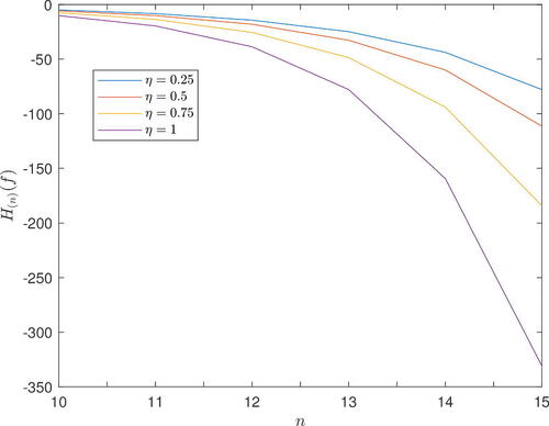
Example 1.

Consider a truncated exponential distribution with parameter η and truncation point x₀ = 0. 5. The pdf is then expressed by $$\begin{array}{l}f(x)=\frac{\eta }{1-\exp (-\eta x_0)}\exp (-\mathrm{\eta x}),x\in [0,x_0].\end{array}$$

For n₀ = 10 and η chosen to be 0. 25, 0. 5, 0. 75, or 1, it is easy to verify that it satisfies the assumption in Corollary 4.1 which guarantees the monotonicity property about the entropies H_(n)(f), as also illustrated in Figure 1.

Figure 1. The values of H_(n)(f) in Example 1 as a function of n.

Remark 3.

Among the different generalizations of Shannon entropy, Tsallis entropy (Tsallis 1988) has attracted considerable attention due to its physical interpretation. With a parameter α > 0, α≠1, it is defined as (21) $$\begin{array}{l}{S}_{\alpha }(f)=\frac{1}{\alpha -1}(1-{\int }_0^{+\mathrm{\infty }}{f}^{\alpha }(x)\mathrm{dx}).\end{array}$$(21)

It is fair to note that (21(21) $$\begin{array}{l}{S}_{\alpha }(f)=\frac{1}{\alpha -1}(1-{\int }_0^{+\mathrm{\infty }}{f}^{\alpha }(x)\mathrm{dx}).\end{array}$$(21) ) was earlier proposed by Burbea and Rao (1982, p. 578). The family of entropies (21(21) $$\begin{array}{l}{S}_{\alpha }(f)=\frac{1}{\alpha -1}(1-{\int }_0^{+\mathrm{\infty }}{f}^{\alpha }(x)\mathrm{dx}).\end{array}$$(21) ) is strictly connected to (19(19) $$\begin{array}{l}{H}_{(\lambda )}(f)=-{\int }_0^{+\mathrm{\infty }}\frac{f^{\lambda +1}(x)-f(x)}{\lambda (\lambda +1)}\mathrm{dx}=-{\int }_0^{+\mathrm{\infty }}\frac{f^{\lambda +1}(x)}{\lambda (\lambda +1)}\mathrm{dx}+\frac{1}{\lambda (\lambda +1)}.\end{array}$$(19) ) as, by choosing $\alpha =\lambda +1$, we have $$\begin{array}{l}{S}_{\lambda +1}(f)=\frac{1}{\lambda }(1-{\int }_0^{+\mathrm{\infty }}{f}^{\lambda +1}(x)\mathrm{dx})=(\lambda +1)H_{(\lambda )}(f),\end{array}$$ for $\lambda >-1$, λ≠0. Consequently, also the extropy, corresponding to λ = 1, is closely related to the Tsallis entropy with parameter α = 2. Another example of one-parameter families of entropies that are linked to C & R is that introduced by Mathai and Haubold (2007) $$\begin{array}{l}{M}_{\alpha }(f)=\frac{1}{1-\alpha }(1-{\int }_0^{+\mathrm{\infty }}{f}^{2-\alpha }(x)\mathrm{dx})=\frac{1-\text{E}[f(x){]}^{1-\alpha }}{1-\alpha },\alpha \ne 1,\alpha <2.\end{array}$$

The authors commented that the larger is the value of 1−α, the larger is the information content and smaller the uncertainlty and vice versa. For this, they called 1−α as the strength of information. We can easily verify that $M_{1-\lambda }(f)=(\lambda +1)H_{(\lambda )}(f)$, for $\lambda >-1$, λ≠0. The families of entropies considered so far are of non-logarithmic scale. The most popular family of logarithmic scaled entropies generalizing the Shannon entropy is the Rényi entropy $$\begin{array}{l}{R}_{\alpha }(f)=\frac{1}{1-\alpha }{\log }_2({\int }_0^{+\mathrm{\infty }}{f}^{\alpha }(x)\mathrm{dx}),\alpha \ne 1,\alpha >0,\end{array}$$ which is also functionally related to the C & R entropy, since $R_{\lambda +1}(f)=\frac{-1}{\lambda }{\log }_2(1-\lambda (\lambda +1)H_{(\lambda )}(f))$, for $\lambda >-1$, λ≠0.

In analogy to (19(19) $$\begin{array}{l}{H}_{(\lambda )}(f)=-{\int }_0^{+\mathrm{\infty }}\frac{f^{\lambda +1}(x)-f(x)}{\lambda (\lambda +1)}\mathrm{dx}=-{\int }_0^{+\mathrm{\infty }}\frac{f^{\lambda +1}(x)}{\lambda (\lambda +1)}\mathrm{dx}+\frac{1}{\lambda (\lambda +1)}.\end{array}$$(19) ), the ϕ-divergene (14(14) $$\begin{array}{l}{D}_{\varphi }(f,g)={\int }_0^{+\mathrm{\infty }}g(x)\varphi \left(\frac{f(x)}{g(x)}\right)\mathrm{dx},\varphi \in {\mathrm{\Phi }}^{\ast }\end{array}$$(14) ) for the functions ϕ_(λ) in (18(18) $$\begin{array}{l}{\varphi }_{(\lambda )}(x)=\frac{x^{\lambda +1}-x}{\lambda (\lambda +1)},\lambda \ne 0,\lambda \ne -1,\end{array}$$(18) ), leads to the one-parameter family of Cressie–Read (C & R) divergences, defined by (22) $$\begin{array}{l}{D}_{(\lambda )}(f,g)={\int }_0^{+\mathrm{\infty }}\frac{g(x)}{\lambda (\lambda +1)}(\frac{f^{\lambda +1}(x)}{g^{\lambda +1}(x)}-\frac{f(x)}{g(x)})\mathrm{dx}=\frac{1}{\lambda +1}{\int }_0^{+\mathrm{\infty }}\frac{f^{\lambda +1}(x)}{g^{\lambda }(x)}\mathrm{dx}-\frac{1}{\lambda +1}.\end{array}$$(22)

For λ→0, D_(λ) converges to the KL divergence (9(9) $$\begin{array}{l}{D}_{\mathrm{KL}}(f,g)={\mathbb{E}}_f[\log \frac{f(X)}{g(X)}]={\int }_0^{+\mathrm{\infty }}f(x)\log \frac{f(x)}{g(x)}\mathrm{dx}.\end{array}$$(9) ) while for λ = 1, it can be shown that D₍₁₎ coincides to the well-known Pearson’s X². Notice that the ϕ-function considered by Pearson (1900) was ${\varphi }_P(x)=\frac{(x-1{)}^2}{2}$. However ϕ_P is a representative of ϕ₍₁₎ (Remark 1 for ϕ = ϕ₍₁₎ and ψ(x) = ϕ_P with $c=-\frac{1}{2}$) and thus D₍₁₎ = D_P. In our context, we use ϕ₍₁₎ and not ϕ_P, since the latter does not define an entropy. An entropy based on ϕ_P would have been expressed as $H_{{\varphi }_P}(f)=-{\int }_0^{+\mathrm{\infty }}\frac{(f(x)-1{)}^2}{2}\mathrm{dx}$, which is always equal to −∞.

5. Extropy as ϕ-entropy

In view of the C & R family of entropies discussed in Section 4, the extropy (2(2) $$\begin{array}{l}J(f)=-\frac{1}{2}{\int }_0^{+\mathrm{\infty }}{f}^2(x)\mathrm{dx}.\end{array}$$(2) ) is directly related to the Pearson entropy (20(20) $$\begin{array}{l}{H}_{(1)}(f)=-{\int }_0^{+\mathrm{\infty }}\frac{f^2(x)-f(x)}{2}\mathrm{dx}.\end{array}$$(20) ), since (23) $$\begin{array}{l}{H}_{(1)}(f)=-\frac{1}{2}{\int }_0^{+\mathrm{\infty }}{f}^2(x)\mathrm{dx}+\frac{1}{2}=J(f)+\frac{1}{2}.\end{array}$$(23)

Analogously, dynamic versions of the extropy are linked to the corresponding Pearson entropies. Thus, the residual and past Pearson entropy are equal to the residual extropy (4(4) $$\begin{array}{ll}{J}^r(f,t)& =-\frac{1}{2{\bar{F}}^2(t)}{\int }_t^{+\mathrm{\infty }}{f}^2(x)\mathrm{dx},\end{array}$$(4) ) and past extropy (6(6) $$\begin{array}{ll}{J}^p(f,t)& =-\frac{1}{2F^2(t)}{\int }_0^t{f}^2(x)\mathrm{dx}.\end{array}$$(6) ), respectively, plus a constant, since (24) $$\begin{array}{ll}{H}_{(1)}^r(f,t)& =-{\int }_t^{+\mathrm{\infty }}{\varphi }_{(1)}\left(\frac{f(x)}{\bar{F}(t)}\right)\mathrm{dx}\\ & =-{\int }_t^{+\mathrm{\infty }}\frac{f^2(x)}{2{\bar{F}}^2(t)}\mathrm{dx}+\frac{1}{2}{\int }_t^{+\mathrm{\infty }}\frac{f(x)}{\bar{F}(t)}\mathrm{dx}=J^r(f,t)+\frac{1}{2}\text{ and}\end{array}$$(24) (25) $$\begin{array}{ll}{H}_{(1)}^p(f,t)& =-{\int }_0^t\frac{f^2(x)}{2F^2(t)}\mathrm{dx}+\frac{1}{2}{\int }_0^t\frac{f(x)}{F(t)}\mathrm{dx}=J^p(f,t)+\frac{1}{2}.\end{array}$$(25)

The same connection holds also between the interval ϕ-entropy (12(12) $$\begin{array}{ll}{H}_{\varphi }^i(f,t_1,t_2)& =-{\int }_{t_1}^{t_2}\varphi \left(\frac{f(x)}{F(t_2)-F(t_1)}\right)\mathrm{dx},\end{array}$$(12) ) for ϕ₍₁₎ and the interval extropy (8(8) $$\begin{array}{ll}{J}^i(f,t_1,t_2)& =-\frac{1}{2(F(t_2)-F(t_1){)}^2}{\int }_{t_1}^{t_2}{f}^2(x)\mathrm{dx}.\end{array}$$(8) ), since (26) $$\begin{array}{l}{H}_{(1)}^i(f,t_1,t_2)=-{\int }_{t_1}^{t_2}\frac{f^2(x)}{2(F(t_2)-F(t_1){)}^2}\mathrm{dx}+\frac{1}{2}{\int }_{t_1}^{t_2}\frac{f(x)}{F(t_2)-F(t_1)}\mathrm{dx}=J^i(f,t_1,t_2)+\frac{1}{2}.\end{array}$$(26)

The expression of extropies in relation to Pearson entropies provides a new insight of extropies and enables the direct transfer of known results for entropies to extropies. Thus, since for given t the residual extropy J^r(f, t) and Pearson residual entropy $H_{(1)}^r(f,t)$ differ only by a constant, they share the same monotonicity properties. For this, Theorem 3.1 for the ϕ-function ϕ₍₁₎, for which $\frac{{\varphi }_{(1)}(x)}{x}=\frac{x-1}{2}$ is non-decreasing in x > 0, directly leads to the following result for the residual extropy.

Corollary 5.1.

Let f be an absolutely continuous pdf with non-increasing (non-decreasing) hazard rate function h_f. Then, the residual extropy is non-decreasing (non-increasing).

Remark 4.

The monotonicity of the residual extropy has already been studied by Qiu and Jia (2018). In fact, they have proved that if f(F⁻¹(x)) is non-decreasing for x > 0, then the residual extropy is non-increasing in t > 0. Actually, the result given in Corollary 5.1 is more general as it requires a less strict assumption. In fact, if f(F⁻¹(x)) is non-decreasing for x > 0, then h_f is non-decreasing. Consider the first derivatives of f(F⁻¹(x)) and h_f(x), $$\begin{array}{l}\frac{d}{\mathrm{dx}}(f(F^{-1}(x)))=\frac{f^{\prime }(F^{-1}(x))}{f(F^{-1}(x))}\\ \text{and }{\text{h}}_f^{\prime }(x)=\frac{f^{\prime }(x)\bar{F}(x)+f^2(x)}{{\bar{F}}^2(x)}.\end{array}$$

Then, for x > 0, f(F⁻¹(x)) is non-decreasing in x if and only if f^′(x)≥0, whereas the hazard rate function h_f is non-decreasing if, and only if, $f^{\prime }(x)\bar{F}(x)+f^2(x)\ge 0$. Being $\bar{F}(x)$ and f²(x) non-negative, from the assumption f^′(x)≥0, it readily follows that h_f is non-decreasing in x > 0. On the contrary, if h_f is non-increasing then f(F⁻¹(x)) is non-increasing but there is no result about the monotonicity of the residual extropy based on such an assumption.

In order to study the monotonicity of a past ϕ-entropy, a result analogous to that of Theorem 3.1 for the residual ϕ-entropy is proven next, based on the reversed hazard rate function $q_f=\frac{f}{F}$.

Theorem 5.1.

Let ϕ be a function such that $\frac{\varphi (x)}{x}$ is non-decreasing in x > 0 and let f be an absolutely continuous pdf. If the reversed hazard rate function q_f is non-increasing, then the past ϕ-entropy $H_{\varphi }^p(f,t)$ is non-decreasing in t > 0.

Proof.

Consider the function $\psi (x)=\frac{\varphi (x)}{x}$ which is non-decreasing by the assumptions. Then, the past ϕ-entropy can be rewritten in terms of ψ as (27) $$\begin{array}{l}{H}_{\varphi }^p(f,t)=-{\int }_0^t\varphi \left(\frac{f(x)}{F(t)}\right)\mathrm{dx}=-{\int }_0^t\frac{f(x)}{F(t)}\psi \left(\frac{f(x)}{F(t)}\right)\mathrm{dx}.\end{array}$$(27)

Now, since the past lifetime ${}_{t}X=(X|X\le t)$ has cdf ${}_{t}F(x)=\frac{F(x)}{F(t)}$ and pdf ${}_{t}f(x)=\frac{f(x)}{F(t)}$ for $x\in (0,t)$, by (27(27) $$\begin{array}{l}{H}_{\varphi }^p(f,t)=-{\int }_0^t\varphi \left(\frac{f(x)}{F(t)}\right)\mathrm{dx}=-{\int }_0^t\frac{f(x)}{F(t)}\psi \left(\frac{f(x)}{F(t)}\right)\mathrm{dx}.\end{array}$$(27) ), it follows $$\begin{array}{l}{H}_{\varphi }^p(f,t)=-{\int }_0^t{}_{t}f(x)\psi {(}_{t}f(x))\mathrm{dx}=-{\int }_0^1\psi {(}_{t}f{(}_t{F}^{-1}(y)))\mathrm{dy},\end{array}$$ where it has been used to change of variable $y={}_{t}F(x)$, such that $\mathrm{dy}={}_{t}f(x)\mathrm{dx}$.

Since the function ψ is non-decreasing, if ${}_{t}f{(}_t{F}^{-1}(y))$ is non-increasing then $H_{\varphi }^p(f,t)$ will be non-decreasing. Recall that for reversed hazard rate function of the past lifetime, we have $$\begin{array}{l}{q}_{{}_{t}f}(x)=\frac{{}_{t}f(x)}{{}_{t}F(x)}=\frac{f(x)}{F(t)}\cdot \frac{F(t)}{F(x)}=q_f(x).\end{array}$$

Then, it readily follows (28) $$\begin{array}{l}{}_{t}f{(}_t{F}^{-1}(y))=\frac{{}_{t}f{(}_t{F}^{-1}(y))}{{}_{t}F{(}_t{F}^{-1}(y))}\cdot {}_{t}F{(}_t{F}^{-1}(y))=q_{{}_{t}f}{(}_t{F}^{-1}(y))\cdot y=q_f{(}_t{F}^{-1}(y))\cdot y.\end{array}$$(28)

Note that the inverse function of the cdf of the past lifetime can be obtained by $$\begin{array}{l}y={}_{t}F(x)=\frac{F(x)}{F(t)},F(x)=\mathrm{yF}(t),x=F^{-1}(\mathrm{yF}(t)).\end{array}$$

Then, from (28(28) $$\begin{array}{l}{}_{t}f{(}_t{F}^{-1}(y))=\frac{{}_{t}f{(}_t{F}^{-1}(y))}{{}_{t}F{(}_t{F}^{-1}(y))}\cdot {}_{t}F{(}_t{F}^{-1}(y))=q_{{}_{t}f}{(}_t{F}^{-1}(y))\cdot y=q_f{(}_t{F}^{-1}(y))\cdot y.\end{array}$$(28) ), it follows $$\begin{array}{l}{}_{t}f{(}_t{F}^{-1}(y))=q_f(F^{-1}(\mathrm{yF}(t)))\cdot y.\end{array}$$

As F and F⁻¹ are non-decreasing, then F⁻¹(yF(t)) is non-decreasing in t > 0. Moreover, q_f is non-increasing and so $q_f(F^{-1}(\mathrm{yF}(t)))\cdot y$ is non-increasing in t > 0 as well. Hence, $H_{\varphi }^p(f,t)$ is non-decreasing and the proof is completed. ▪ ▪

Remark 5.

The result of Theorem 5.1 for the function ϕ₍₁₎, which corresponds to the monotonicity of the past extropy, follows as a corollary of Theorem 2.3 in Kamari and Buono (2021). There it is stated that if f(F⁻¹(x)) is non-increasing in x > 0, then the past extropy J^p(f, t) is non-decreasing in t > 0. Note that by considering the function ϕ₍₁₎, the hypothesis about the monotonicity of $\frac{\varphi (x)}{x}$ is satisfied. In addition, if $f(F^{-1}(\cdot ))$ is non-increasing then the reversed hazard rate function q_f(⋅) is non-increasing. In fact $$\begin{array}{l}\frac{d}{\mathrm{dx}}f(F^{-1}(x))=\frac{f^{\prime }(F^{-1}(x))}{f(F^{-1}(x))}\le 0⟺f^{\prime }(\cdot )\le 0,\end{array}$$ and the first derivative of the reversed hazard rate function is expressed as $$\begin{array}{l}{q}_f^{\prime }(x)=\frac{f^{\prime }(x)F(x)-f^2(x)}{F^2(x)},\end{array}$$ which is non-positive by assuming that $f^{\prime }(\cdot )\le 0$.

Remark 6.

In analogy with Theorem 3.1, it may seem of interest to consider Theorem 5.1 also for a non-decreasing reversed hazard rate function. But, as our purpose is to apply the results to non-negative random variables, this case is not of interest since there do not exist non-negative random variables with non-decreasing reversed hazard rate function (see Block, Savits, and Singh 1998). In addition, note that it is not possible to derive results similar to Corollary 5.1 and Theorem 5.1 related to the interval ϕ-entropy. In fact, the hazard and the reversed hazard rate function of a doubly truncated random variable are not equal to the ones of the original random variable, as it happens for the former and the residual life and for the latter and the past lifetime.

Remark 7.

The dynamic ϕ-divergence versions obtained with the function ϕ₍₁₎, provide the expressions for the divergences comparing the corresponding Pearson entropies of two densities. In particular, from (15(15) $$\begin{array}{ll}{D}_{\varphi }^r(f,g,t)& ={\int }_t^{+\mathrm{\infty }}\frac{g(x)}{\bar{G}(t)}\varphi (\frac{f(x)}{g(x)}\cdot \frac{\bar{G}(t)}{\bar{F}(t)})\mathrm{dx},\end{array}$$(15) ), we get the residual Pearson entropy divergence $$\begin{array}{l}{D}_{(1)}^r(f,g;t)={\int }_t^{+\mathrm{\infty }}\frac{g(x)}{\bar{G}(t)}{\varphi }_{(1)}(\frac{f(x)}{g(x)}\cdot \frac{\bar{G}(t)}{\bar{F}(t)})\mathrm{dx}=\frac{1}{2}{\int }_t^{+\mathrm{\infty }}\frac{f^2(x)}{g(x)}\cdot \frac{\bar{G}(t)}{{\bar{F}}^2(t)}\mathrm{dx}-\frac{1}{2}.\end{array}$$

Similar expression can be obtained for the interval Pearson entropy divergence and the past Pearson entropy divergence from (16(16) $$\begin{array}{ll}{D}_{\varphi }^i(f,g,t_1,t_2)& ={\int }_{t_1}^{t_2}\frac{g(x)}{G(t_2)-G(t_1)}\varphi (\frac{f(x)}{g(x)}\cdot \frac{G(t_2)-G(t_1)}{F(t_2)-F(t_1)})\mathrm{dx},\end{array}$$(16) ) and (17(17) $$\begin{array}{ll}{D}_{\varphi }^p(f,g,t)& ={\int }_0^t\frac{g(x)}{G(t)}\varphi (\frac{f(x)}{g(x)}\cdot \frac{G(t)}{F(t)})\mathrm{dx}.\end{array}$$(17) ), respectively. Note that the function ϕ₍₁₎ has a non-decreasing representative ($\psi (x)=\frac{x^2-1}{2}$), so that the results in Theorem 3.2 and 3.3 can be applied to the residual Pearson entropy divergence.

Due to the connection between the corresponding Pearsonian entropy and extropy expressions (24(24) $$\begin{array}{ll}{H}_{(1)}^r(f,t)& =-{\int }_t^{+\mathrm{\infty }}{\varphi }_{(1)}\left(\frac{f(x)}{\bar{F}(t)}\right)\mathrm{dx}\\ & =-{\int }_t^{+\mathrm{\infty }}\frac{f^2(x)}{2{\bar{F}}^2(t)}\mathrm{dx}+\frac{1}{2}{\int }_t^{+\mathrm{\infty }}\frac{f(x)}{\bar{F}(t)}\mathrm{dx}=J^r(f,t)+\frac{1}{2}\text{ and}\end{array}$$(24) )–(26(26) $$\begin{array}{l}{H}_{(1)}^i(f,t_1,t_2)=-{\int }_{t_1}^{t_2}\frac{f^2(x)}{2(F(t_2)-F(t_1){)}^2}\mathrm{dx}+\frac{1}{2}{\int }_{t_1}^{t_2}\frac{f(x)}{F(t_2)-F(t_1)}\mathrm{dx}=J^i(f,t_1,t_2)+\frac{1}{2}.\end{array}$$(26) ), one would expect that extropy-based divergences can be defined. For example, the residual extropy divergence would have been $D_{\mathrm{ex}}^r(f,g;t)=D_{(1)}^r(f,g;t)+1/2$. However, this is not possible, since the ϕ-function used for the definition of the extropy, $\varphi (x)=x^2/2$ does not belong to Φ^* (ϕ(1)≠0) and thus cannot be used for defining a divergence.

6. Examples

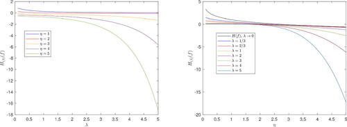
Example 2.

Consider an exponential distribution with parameter η > 0, $f(x)=\eta e^{-\mathrm{\eta x}}$, x≥0. Then, the generalized ϕ-entropy H_(λ)(f) is obtained as $$\begin{array}{rlr}{H}_{(\lambda )}(f)& =& -{\int }_0^{+\mathrm{\infty }}\frac{{\eta }^{\lambda +1}{e}^{-\eta (\lambda +1)x}}{\lambda (\lambda +1)}\mathrm{dx}+\frac{1}{\lambda (\lambda +1)}=-\frac{{\eta }^{\lambda }}{\lambda (\lambda +1{)}^2}+\frac{1}{\lambda (\lambda +1)}.\end{array}$$

In Figure 2 (left), we plot the generalized entropy as a function of λ for representative fixed values of the parameter of the exponential distribution, while in Figure 2 (right), we fix the parameter λ and consider H_(λ)(f) as a function of the parameter of the exponential distribution η. The Shannon entropy H(f), which corresponds to the limiting case λ→0, is also pictured. In both cases, we can observe a decreasing behavior in terms of λ or η. Moreover, in analogy with the classical continuous version of entropy, the generalized entropy H_(λ)(f) is not always positive. In particular, the points in which there is a sign change in terms of η, with fixed λ, are reported in Table 2. There we can observe a decreasing nature of these change-sign points, which corresponds to a smaller region of the parameter space in which the entropy is non-negative.

Table 2. Values of η for fixed λ such that H_(λ)(f) = 0 where f is the pdf of an exponential distribution.

λ	→0	1/3	2/3	1	2	3	4	5
η	e	2.3704	2.1517	2	1.7321	1.5874	1.4953	1.4310

Figure 2. Generalized entropy for exponential distribution in Example 2, plotted as a function of λ with fixed η on the left, and vice versa on the right.

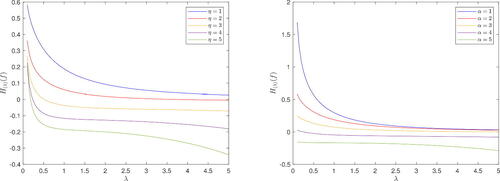
Example 3.

Consider a Weibull distribution with parameters α and η, with pdf $f(x)=\mathrm{\alpha \eta }{x}^{\alpha -1}\exp (-\eta x^{\alpha })$, x≥0. In this case, we cannot evaluate analytically the expression of the generalized ϕ-entropies H_(λ), but they can be computed numerically. In Figure 3, H_(λ)(f) is plotted as a function of λ with a fixed value of α = 2 and different choices for η, on the left, and a fixed value of η = 1 and different choices for α, on the right.

Figure 3. Generalized entropy for Weibull distribution in Example 3, plotted as a function of λ with fixed α = 2 and different choices for η on the left, and fixed η = 1 and different choices for α on the right.

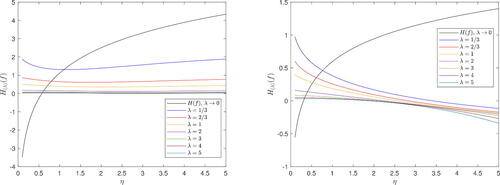
In Figure 4, H_(λ)(f) is plotted as a function of η by keeping fixed α = 0. 5 (on the left) or α = 2 (on the right), and with different choices for the parameter λ. The limiting case for λ→0 (Shannon entropy) is also included in these graphs. We observe a completely different behavior of the Shannon entropy with respect to the generalized versions of entropy. Moreover, in Figure 4 (left) there are some cases of non-monotonic generalized entropies.

Figure 4. Generalized entropy for Weibull distribution in Example 3, plotted as a function of η with fixed α = 0. 5 (left) or α = 2 (right) and different choices for λ.

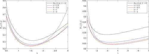
Next, we make some comparisons between Weibull and exponential distributions by using generalized divergences (the results can be computed only numerically). Consider a Weibull pdf with parameters α and γ, $f(x)=\mathrm{\alpha \gamma }{x}^{\alpha -1}\exp (-\gamma x^{\alpha })$, x > 0 and an exponential pdf with parameter η, $g(x)=\mathrm{\eta exp}(-\mathrm{\eta x})$, x > 0. In order to have a finite divergence of f from g, D_(λ)(f, g), we need α to be greater than 1. In this example, it will be fixed to 2. Note that if we want to consider the divergence of g from f, that is, D_(λ)(g, f), α needs to be less than 1. In Figure 5, the generalized divergence is plotted as a function of η with fixed γ = 2 (left), and as a function of γ with fixed η = 2 (right), for a selection of λ values, including the limiting case λ→0, which corresponds to D_KL(f, g). The values of η and γ, for which the divergence values in Figure 5 reach their minimum, are given in Table 3.

Table 3. Values of η and γ for which the divergences in Figure 5 reach the minimum value.

λ	→0 (KL)	1/3	2/3	1	2
η	1.5606	1.5354	1.5101	1.4848	1.5606	Figure 5 (left)
γ	2.9394	3.3030	3.3636	3.4848	3.6061	Figure 5 (right)

Figure 5. Generalized divergence for exponential and Weibull distributions in Example 3, plotted as a function of η with fixed γ = 2 on the left, and vice versa on the right.

Example 4.

Consider a real data set (see Data Set 4.1 in Murthy, Xie, and Jiang 2004) presenting times to failure of 20 units: $$\begin{array}{l}11.24,1.92,12.74,22.48,9.60,11.50,8.86,7.75,5.73,9.37,\end{array}$$ $$\begin{array}{l}30.42,9.17,10.20,5.52,5.85,38.14,2.99,16.58,18.92,13.36.\end{array}$$

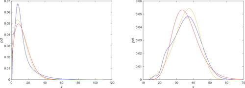
Suppose the data are distributed as a random variable X with pdf f. The probability density function can be estimated by a kernel estimator (e.g., with MATLAB function ksdensity). In order to establish if the distribution of the data is similar to a Weibull distribution W2(α, λ) with pdf g, we consider two different Weibull distribution, $Y_1\sim W2(1.5487,0.0166)$, with parameters given by the maximum likelihood method, and Y₂∼ W2(1. 6, 0. 0127), already considered in Balakrishnan et al. (2023). We remark that both distributions are accepted by applying the Kolmogorov-Smirnov test at a significance level of 5%. In Figure 6 (left), the estimated pdf of the data and the pdf’s g₁, g₂ of Y₁, Y₂ are plotted.

Figure 6. Plot of pdf’s of X (estimated), Y₁ and Y₂ in Example 4 (left) and in Example 5 (right) (blue, yellow and red lines, respectively).

As already pointed out in Balakrishnan et al. (2023), with these distributions we have the same value of KL divergence, $$\begin{array}{l}{D}_{\mathrm{KL}}(f,g_1)=D_{\mathrm{KL}}(f,g_2)=0.0990.\end{array}$$

Hence, to choose the more suitable distribution, an additional criterion was used in Balakrishnan et al. (2023), based on a dispersion index of KL divergence, bringing to choose Y₂. Here, we use the generalized divergences D_(λ)(f, g) to make comparisons among Y₁ and Y₂ with different choices of the parameter λ. We find out that Y₂ performs better than Y₁, that is, it has lower measures of divergence, for λ > 0 with growing difference in λ. The results are presented in Table 4 for some selected choices of λ. Hence, by using generalized divergences, we are able to overcome the problem of equal KL divergences and our results are consistent with the method proposed in Balakrishnan et al. (2023).

Table 4. Values of D_(λ)(f, g₁) and D_(λ)(f, g₂) in Example 4 for different choices of λ.

λ	0.1	1/3	1/2	2/3	3/4	1	2
D(λ)(f, g1)	0.0950	0.1553	0.2710	0.6702	1.2129	10.8589	6.0464e+05
D(λ)(f, g2)	0.0924	0.1380	0.2170	0.4712	0.7985	6.0010	1.8342e+05

Example 5.

Consider the crab dataset presented in Murphy and Aha (1994). We focus our attention on the distribution of the width of female crabs, represented by the random variable X with pdf f, so that we have a sample of 100 units. As in Example 4, we first estimate the probability density function through a kernel estimator with MATLAB function ksdensity. We now wish to compare the distribution of the data with Weibull and Lognormal distributions. By using the maximum likelihood estimation, we choose Y₁∼W2(5. 6162, 1. 1953e-09) and $Y_2\sim \mathrm{Lognormal}(3.5559,0.2192)$. We recall that if $Y_2\sim \mathrm{Lognormal}(\mu ,\sigma )$, then the pdf is $g_2(x)=\frac{1}{\mathrm{x\sigma }\sqrt{2\pi }}\exp (-\frac{(\log x-\mu {)}^2}{2{\sigma }^2})$, x > 0. Note that both distributions are accepted by using the Kolmogorov-Smirnov test at a significance level of 5%. In Figure 6 (right), the estimated pdf of the data and the pdf’s of Y₁, Y₂ are plotted. The comparison among these two distributions has been already performed in Balakrishnan et al. (2023), where the values of KL divergence were computed as $D_{\mathrm{KL}}(f,g_1)=0.0381$ and $D_{\mathrm{KL}}(f,g_2)=0.0420$. Although D_KL(f, g₁) is lower than D_KL(f, g₂), it can be noted that the values are similar and really close to zero. Hence, in that paper, they used an additional criterion, which brought to choose Y₂ instead of Y₁ by tolerating a slightly greater value of KL divergence. Now, we use the generalized divergences D_(λ)(f, g) to make comparisons among Y₁ and Y₂ with different choices of the parameter λ. We find out that for λ > λ₀ (λ₀≃0. 185), Y₂ starts to perform much better than Y₁, i.e., it has lower measures of divergence with growing difference by increasing the value of λ. In particular for λ₀ we have $D_{({\lambda }_0)}(f,g_1)=D_{({\lambda }_0)}(f,g_2)\simeq 0.0430$. The results are presented in Table 5 for some selected choices of λ. Hence, by using generalized divergences, we are able to overcome the problem of almost equal values of KL divergences and our results are consistent with the method proposed in Balakrishnan et al. (2023).

Table 5. Values of D_(λ)(f, g₁) and D_(λ)(f, g₂) in Example 5 for different choices of λ.

λ	0.1	1/3	1/2	2/3	3/4	1	3/2	2
D(λ)(f, g1)	0.0402	0.0503	0.0672	0.1122	0.1632	0.8296	73.8981	1.1360e+04
D(λ)(f, g2)	0.0423	0.0444	0.0464	0.0491	0.0507	0.0569	0.0803	0.1351

7. Conclusion

Parametric families of entropies and associated divergences, generalizing Shannon’s entropy and the Kullback-Leibler (KL) divergence, respectively, play a predominant role in diverse scientific fields, ranging from physics to econometrics and reliability. In this article, we have discussed the concepts of generalized entropies and divergences with their corresponding dynamic versions, which are of special interest in reliability. We showed off that they introduce a kind of scale in measuring entropy. For example, focusing in the Cressie and Read (C & R) family of entropies, if there is a rough prior information about the area of value of η, we can decide for the scale (through the C & R parameter λ) in order to control the level of entropy (see Figure 2). We also linked the dual measure of Shannon entropy, namely the extropy, to the ϕ-entropies generated by the C & R ϕ-functions by proving that the extropy is a member of the C & R family of entropies. We provided several examples of generalized entropies for representative lifetime distributions to highlight the effect of the distributions’ parameter values and of the C & R parameter λ. Finally, the generalized divergences are employed for deciding on the distribution underlying real data in two examples. We verified in both cases that specific λ-values performed better than the well-known KL divergence. In reliability applications, various types of censoring often occur. In future research, it would be of interest to investigate the properties of generalized entropies and divergences under censoring. Furthermore, the extension of the study under assumptions corresponding to different reliability aging classes may lead to new results for the associated residual, past and interval measures.

Acknowledgments

FB is member of the research group GNAMPA of INdAM (Istituto Nazionale di Alta Matematica).

Disclosure statement

No potential conflict of interest was reported by the author(s).

References

- Ali, S. M., and S. D. Silvey. 1966. A general class of coefficients of divergence of one distribution from another. Journal of the Royal Statistical Society Series B: Statistical Methodology 28 (1):131–42. doi:10.1111/j.2517-6161.1966.tb00626.x.
- Amigó, J., S. Balogh, and S. Hernández. 2018. A brief review of generalized entropies. Entropy 20 (11):813. doi:10.3390/e20110813.
- Arizono, I, and H. Ohta. 1989. A test for normality based on Kullback-Leibler information. The American Statistician 43 (1):20–2. doi:10.1080/00031305.1989.10475600.
- Balakrishnan, N., F. Buono, C. Calí, and M. Longobardi. 2023. Dispersion indices based on Kerridge inaccuracy measure and Kullback-Leibler divergence. Communications in Statistics - Theory and Methods 53 (15):5574–92. doi:10.1080/03610926.2023.2222926.
- Balakrishnan, N., A. H. Rad, and N. R. Arghami. 2007. Testing exponentiality based on Kullback-Leibler information with progressively Type-II censored data. IEEE Transactions on Reliability 56:349–56.
- Block, H. W., T. H. Savits, and H. Singh. 1998. The reversed hazard rate function. Probability in the Engineering and Informational Sciences 12 (1):69–90. doi:10.1017/S0269964800005064.
- Buono, F., O. Kamari, and M. Longobardi. 2023. Interval extropy and weighted interval extropy. Ricerche Di Matematica 72 (1):283–98. doi:10.1007/s11587-021-00678-x.
- Burbea, J. 1984. The Bose-Einstein entropy of degree alpha and its Jensen difference. Utilitas Mathematicas 25:225–40.
- Burbea, J., and C. Rao. 1982. Entropy differential metric, distance and divergence measures in probability spaces: A unified approach. Journal of Multivariate Analysis 12 (4):575–96. doi:10.1016/0047-259X(82)90065-3.
- Cressie, N., and T. R. Read. 1984. Multinomial goodness-of-fit tests. Journal of the Royal Statistical Society Series B: Statistical Methodology 46 (3):440–64. doi:10.1111/j.2517-6161.1984.tb01318.x.
- Cumming, S. G. 2001. A parametric model of the fire-size distribution. Canadian Journal of Forest Research 31 (8):1297–303. doi:10.1139/x01-032.
- Devarajan, K., G. Wang, and N. Ebrahimi. 2015. A unified statistical approach to non-negative matrix factorization and probabilistic latent semantic indexing. Machine Learning 99 (1):137–63. doi:10.1007/s10994-014-5470-z. 25821345
- Di Crescenzo, A., and M. Longobardi. 2002. Entropy-based measure of uncertainty in past lifetime distributions. Journal of Applied Probability 39 (2):434–40. doi:10.1239/jap/1025131441.
- Di Crescenzo, A., and M. Longobardi. 2009. On cumulative entropies. Journal of Statistical Planning and Inference 139 (12):4072–87. doi:10.1016/j.jspi.2009.05.038.
- Crescenzo, A. D., and M. Longobardi. 2015. Some properties and applications of cumulative Kullback–Leibler information. Applied Stochastic Models in Business and Industry 31 (6):875–91. doi:10.1002/asmb.2116.
- Ebrahimi, N. 1996. How to measure uncertainty in the residual life time distribution. Sankhyoverlinea: Series A 58:48–56.
- Ebrahimi, N., and S. Kirmani. 1996. A measure of discrimination between two residual life-time distributions and its applications. Annals of the Institute of Statistical Mathematics 48 (2):247–65.
- Espendiller, M., and M. Kateri. 2016. A family of association measures for 2 × 2 contingency tables based on the ϕ-divergence. Statistical Methodology 30:45–61. doi:10.1016/j.stamet.2015.12.002.
- Hashempour, M., M. R. Kazemi, and S. Tahmasebi. 2022. On weighted cumulative residual extropy: characterization, estimation and testing. Statistics 56 (3):681–98. doi:10.1080/02331888.2022.2072505.
- Havrda, J., and F. Charvat. 1967. Concept of structural alpha-entropy. Kybernetika 3:30–5.
- Iranpour, M., M. A. Hejazi, and M. Shahidehpour. 2020. A unified approach for reliability assessment of critical infrastructures using graph theory and entropy. IEEE Transactions on Smart Grid 11 (6):5184–92. doi:10.1109/TSG.2020.3005862.
- Kamari, O., and F. Buono. 2021. On extropy of past lifetime distribution. Ricerche Di Matematica 70 (2):505–15. doi:10.1007/s11587-020-00488-7.
- Kang, H. Y, and B. M. Kwak. 2009. Application of maximum entropy principle for reliability-based design optimization. Structural and Multidisciplinary Optimization 38 (4):331–46. doi:10.1007/s00158-008-0299-3.
- Kapur, J. N. 1972. Measures of uncertainty, mathematical programming and physics. Journal of the Indian Society of Agriculture and Statistics 24:47–66.
- Khinchin, A. I. 1957. Mathematical foundations of information theory. New York: Dover Publications.
- Klein, I., and M. Doll. 2020. (Generalized) maximum cumulative direct, residual, and paired Φ entropy approach. Entropy 22 (1):91. doi:10.3390/e22010091.
- Kullback, S., and R. A. Leibler. 1951. On information and sufficiency. The Annals of Mathematical Statistics 22 (1):79–86. doi:10.1214/aoms/1177729694.
- Lad, F., G. Sanfilippo, and G. Agrò. 2015. Extropy: Complementary dual of entropy. Statistical Science 30:40–58.
- Liese, F., and I. Vajda. 1987. Convex statistical distances. Leipzig: Teubner.
- Maasoumi, E., and J. Racine. 2002. Entropy and predictability of stock market returns. Journal of Econometrics 107 (1-2):291–312. doi:10.1016/S0304-4076(01)00125-7.
- Mathai, A. M., and H. J. Haubold. 2007. Pathway model, superstatistics, Tsallis statistics, and a generalized measure of entropy. Physica A: Statistical Mechanics and Its Applications 375 (1):110–22. doi:10.1016/j.physa.2006.09.002.
- Melbourne, J., S. Talukdar, S. Bhaban, M. Madiman, and M. V. Salapaka. 2022. The differential entropy of mixtures: new bounds and applications. IEEE Transactions on Information Theory 68 (4):2123–46. doi:10.1109/TIT.2022.3140661.
- Mohammadi, M., and M. Hashempour. 2022. On interval weighted cumulative residual and past extropies. Statistics 56 (5):1029–47. doi:10.1080/02331888.2022.2111429.
- Morimoto, T. 1963. Markov processes and the H-theorem. Journal of the Physical Society of Japan 18 (3):328–31. doi:10.1143/JPSJ.18.328.
- Murphy, P. M., and D. W. Aha. 1994. UCI Repository of machine learning databases. Berkeley, CA: University of California, Department of Information and Computer Science, http://www.ics.uci.edu/mlearn/MLRepository.html.Irvine.
- Murthy, D. N. P.,M. Xie, and R. Jiang, 2004. Weibull models. Hoboken, NJ: John Wiley & Sons.
- Pape, N. T. 2015. Phi-divergences and dynamic entropies for quantifying uncertainty in lifetime distributions. M.Sc. thesis, Aachen, Germany: Department of Mathematics, RWTH Aachen University.
- Pardo, L. 2005. Statistical inference based on divergence measures. Boca Raton, FL: Chapman and Hall/CRC.
- Pearson, K. 1900. X. On the criterion that a given system of deviations from the probable in the case of a correlated system of variables is such that it can be reasonably supposed to have arisen from random sampling. The London, Edinburgh, and Dublin Philosophical Magazine and Journal of Science 50 (302):157–75. doi:10.1080/14786440009463897.
- Qiu, G., and Kai. Jia. 2018. The residual extropy of order statistics. Statistics & Probability Letters 133:15–22. doi:10.1016/j.spl.2017.09.014.
- Rao, M., Y. Chen, B. C. Vemuri, and F. Wang. 2004. Cumulative residual entropy: A new measure of information. IEEE Transactions on Information Theory 50 (6):1220–8. doi:10.1109/TIT.2004.828057.
- Raschke, M. 2012. Inference for the truncated exponential distribution. Stochastic Environmental Research and Risk Assessment 26 (1):127–38. doi:10.1007/s00477-011-0458-8.
- Ruggeri, F., M. Sánchez-Sánchez, M. Á. Sordo, and A. Suárez-Llorens. 2021. On a new class of multivariate prior distributions: Theory and application in reliability. Bayesian Analysis 16:31–60.
- Shannon, C. E. 1948. A mathematical theory of communication. Bell System Technical Journal 27 (3):379–423. doi:10.1002/j.1538-7305.1948.tb01338.x.
- Sheikh, A. K., J. K. Boah, and M. Younas. 1989. Truncated extreme value model for pipeline reliability. Reliability Engineering & System Safety 25 (1):1–14. doi:10.1016/0951-8320(89)90020-3.
- Shi, X., A. P. Teixeira, J. Zhang, and C. Guedes Soares. 2014. Structural reliability analysis based on probabilistic response modelling using the Maximum Entropy Method. Engineering Structures 70:106–16. doi:10.1016/j.engstruct.2014.03.033.
- Singh, V. B., M. Sharma, and H. Pham. 2018. Entropy based software reliability analysis of multi-version open source software. IEEE Transactions on Software Engineering 44 (12):1207–23. doi:10.1109/TSE.2017.2766070.
- Soofi, E. S. 1994. Capturing the intangible concept of information. Journal of the American Statistical Association 89 (428):1243–54. doi:10.1080/01621459.1994.10476865.
- Soofi, E. S. 2000. Principal information theoretic approaches. Journal of the American Statistical Association 95 (452):1349 doi:10.2307/2669786.
- Sunoj, S. M., P. G. Sankaran, and S. S. Maya. 2009. Characterizations of life distributions using conditional expectations of doubly (interval) truncated random variables. Communications in Statistics - Theory and Methods 38 (9):1441–52. doi:10.1080/03610920802455001.
- Tsallis, C. 1988. Possible generalization of Boltzmann-Gibbs statistics. Journal of Statistical Physics 52 (1-2):479–87. doi:10.1007/BF01016429.
- Weijs, S. V., R. Van Nooijen, and N. Van De Giesen. 2010. Kullback–Leibler divergence as a forecast skill score with classic reliability–resolution–uncertainty decomposition. Monthly Weather Review 138 (9):3387–99. doi:10.1175/2010MWR3229.1.