Genotype-by-environment interaction analysis for cotton seed yield using various biometrical methods under irrigation regimes in a semi-arid region

ABSTRACT

The main objective of this study was to identify high-yielding and stable cotton genotypes under normal irrigation regimes and drought stress conditions using some biometrical methods including combined analysis of variance (ANOVA), joint regression analysis (JRA), the additive main effect and multiplicative interaction (AMMI), and genotype (G) main effect plus genotype-by-environment (GE) interaction (GGE) biplot. Cotton seed yield (CSY) was found to be significantly affected by genotypes, environments, and Genotype-by-environment interaction (GEI) using combined ANOVA, JRA, and AMMI. AMMI was superior, explaining 79% of the total variability caused by GEI under drought stress conditions compared to 66% and 25% for the GGE biplot and JRA, respectively. The CSY was found to be significantly lower under drought stress conditions vs normal irrigation regimes, ranging from 9.03% (G24) to 29.91% (G15) across the five tested environments. The JRA, AMMI, and GGE biplot methods were positively correlated for classifying the genotypes for static stability. The GGE biplot was the most effective and acceptable for identifying stable genotypes and optimal environments in both irrigation regimes. All the methods compared were concordant in separating, ranking, and identifying that the G5 and G20 genotypes were highly stable across the environment as being higher-yielding and drought-tolerant.

KEYWORDS:

• Drought stress
• GGE biplots
• joint regression analysis
• AMMI models
• multi-environmental trials

Introduction

Many agricultural regions of the world are experiencing a scarcity of irrigation water, which limits the global production of agricultural crops (Ghaed-Rahimi et al. 2014; El Sherbiny et al. 2022). With the increased demand from industry and urban consumption, irrigation water became an essential, limited, and expensive commodity all over the world (Rosa et al. 2020). Hence, great care must be taken when formulating solutions to decrease irrigation water losses and increase crop water productivity, particularly in semi-arid climates of the world (Rao et al. 2016; Mekdad et al. 2021a; Shaaban et al. 2022, 2023; El-Hashash et al. 2022). There is a growing impetus to develop high-yielding and stable genotypes of various field crops with better water productivity and resilience to frequent and prolonged drought stress.

Cotton is the most important and natural textile fiber crop all over the world and is locally an important crop for the industry in Egypt (USDA-ERS 2020). Cotton is commonly known as ‘white gold’, due to its important role in industrial development (fiber and oil) and employment generation (Ahmed and Delin 2019). Environmental factors (non-genetic factors) such as locations, growing seasons or years, drought conditions, the amount of precipitation received in each season, temperature, etc. may have positive or negative effects on genotypes (El-Hashash et al. 2018). Exploring the possibilities of drought-tolerant crops is the time required for all terrestrial crop species, especially under future climate change scenario (El-Hashash and Agwa 2018). Drought tolerance is defined as the relative genotype yield under water limitation compared to its yield under irrigated conditions (Hall 1993), and the plant capacity in withstanding the periods of dryness which is related to phenotypic, morphological, and physiological factors (Yan et al. 2012). The relatively higher yield performance of genotypes under drought and normal irrigated conditions seems to be a good starting point in the identification of traits related to drought tolerance and the selection of genotypes for use in breeding for dry environments (Clarke et al. 1992).

The main target of plant breeding programs is to increase stability and stabilize crop yield across environments (locations and/or years). The yield performances of genotypes could differ significantly when they are assessed over different environments (Ebem et al. 2021). A genotype or the genetic makeup of an organism is defined as a combination of alleles at a single autosomal locus in a diploid organism (Falconer and Mackay 1996). The phenotypic expression of an individual is determined by both genotype and environmental effects (Falconer and Mackay 1996), and phenotypes can be observed, measured, classified, or counted. A change in the relative performance of a ‘trait’ of two or more genotypes assessed in two or more environments is known as a genotype × environment interaction (GEI) according to Bowman (1972). The GEI is a common phenomenon or routine occurrence in plant breeding programs (Kang 1998), which resulting from changes in the magnitude of differences among genotypes in different environments or due to changes in the relative ranking of the genotypes (Ebdon and Gauch 2002), also from one environment to the next, or a difference in scale between environments, or a combination of the two together (Mohammadi and Amri 2008). Evaluation and understanding of the GEI are two major steps towards the development of improved crop genotypes (Sabri et al. 2020). So, cotton breeders must consider GEI while developing genotypes under drought stress conditions. Where the GEI determines the adaptability of a genotype for an entire range of environmental conditions or separate genotypes must be selected for different sub environments (McKeand et al. 1990). To account for GEI effects, the breeders evaluate genotypes in several environments (years and locations) to identify those with high and stable performance with better adaptability (Yan et al. 2000). Genotypes with insignificant GEI are considered to be best due to their better stability (Ssemakula and Dixon 2007). GEI has become a major challenge for crop breeding efforts (Zobel and Talbert 1984) in the discovery of superior genotypes, if genotypes cultivated in different settings have varied relative performances (Allard and Bradshaw 1964). Also, it becomes a potentially valuable tool for developing crops in a specific geographic region (Alizadeh et al. 2017), especially under drought stress conditions. Several statistical modeling tools, one used by biometricians can be used for evaluating and interpreting GEI. Among these methods, joint regression analysis (JRA), the additive main effect and multiplicative interaction (AMMI) model and genotype (G) main effect plus genotype-by-environment (GE) interaction (GGE) biplot.

The linear regression of genotype values on environmental mean yield is known as JRA. In crop sciences, JRA has been widely utilized to structure and understand GEI (Finlay and Wilkinson 1963; Eberhart and Russell 1966; Perkins and Jinks 1968). Due to its simplicity and adaptive responses, it is easily applicable to locations other than the chosen test sites and is undoubtedly the most popular one (Romagosa and Fox 1993). Under a multi-environment trial dataset, the AMMI model merged analysis of variance (ANOVA) and principal component analysis (PCA) into an integrated approach (Zobel et al. 1988; Gauch and Zobel 1997; Gauch 2013). The AMMI model enables the description of genotypical and environmental main effects by ANOVA (an additive model) and characterizes residual GEI (IPCA) and genotypes stability analysis by PCA (a multiplicative model). The AMMI model has been widely utilized to analyze multi-environment yield trials for two main reasons: to better comprehend complicated GEI and to increase accuracy (Gauch 2013). Yan et al. (2000) introduced the GGE biplot methodology, which is a sophisticated statistical model that addresses some of the AMMI model disadvantages. The GGE biplot has proven to be very effective, and more comprehensive approach for analyzing GEI in different mega environments in quantitative genetics and plant breeding (Yan and Rajcan 2002; Yan et al. 2007). The GGE biplot combines two important sources of variation in mega environments (Genotype and G × E), thus the name GGE. Also, it is utilized for mega environment analysis (Which-Won-Where pattern), genotype evaluation (ranking biplot), and environment evaluation (comparison biplot), hence the name GGE biplot, which provides discriminating power and environment representation (Yan and Tinker 2006).

Several reviews have compared the statistical methods of JRA, AMMI model and GGE biplot with respect to their suitability for GE interaction analysis.These comparisons were in pairs or all three together (Yau 1995; Acciaresi et al. 1997; Annicchiarico 1997; Ding et al. 2008; Gauch et al. 2008; Alwala et al. 2010; Rodrigues et al. 2011; Oliveira et al. 2012; Alizadeh et al. 2017; Rana et al. 2021). In mega environment analysis and genotype evaluation, both GGE biplot and AMMI analysis combine rather than separate G and GE (Yan et al. 2007). These two methods differ in that GGE biplot analysis is based on environment-centered PCA, while AMMI analysis is based on double-centered PCA (Kroonenberg 1995). The GGE biplot outperforms AMMI in terms of visual interpretations, particularly the ability to visualize any crossover G × E interaction. This aspect of G × E interaction is typically critical to a breeding program (Ding et al. 2008). The main study objectives were to assess the effect of GEI, genotype stability, and test environment evaluation of cotton seed yield, as well as identify high-yielding and stable cotton genotypes grown under normal irrigation regimes and drought stress conditions using several biometrical methods.

Materials and methods

Genetic material, experimental design, and test environments

The current study was conducted at Sakha Agriculture Research Station (31° 30′ 7.59′′ and 31° 9′ 58.09′′ N and between 30° 20′ 36.83′′ and 31° 17′ 15.16 E) located at the Kafr El-Sheikh Governorate, Egypt, from 2016 to 2020 growing summer seasons. A total of twenty-four Egyptian cotton (Gossypium barbadense L.) genotypes were chosen for this study from different origins as listed in Table S1. The experimental cotton genotype seeds were provided by the Cotton Research Institute, Agriculture Research Center, Giza, Egypt. These genotypes were separately assessed by randomly distributing in a random complete block design with three replications under normal irrigation regime and drought stress conditions (i.e. 100% and 60% of crop evapotranspiration, respectively) conditions during five successive test environments.

Experimental locations and agricultural practices

The experimental location is described as an arid agro-environment with very low seasonality precipitations (less than 10 mm). The monthly average temperature (^◦C), precipitation (mm), and average relative humidity (%) during the experimental period (May to October) for the five tested growing seasons (2016 to 2020) are shown in Figure S1. The highest precipitation and relative humidity, and the lowest average temperature during the experimental period were recorded in April of both 2017 and 2020 growing seasons. Seeds of each tested genotype were hand sown with 0.7 m inter-row spacing and 0.3 m intra-row spacing in each experimental plot. Each experimental plot included five rows of 4 m long and 0.7 m width, forming a 14 m² net plot area. Plots were over-sown with tested cotton genotype seeds and followed by manually thinning to maintain two healthy plants per hill (Mekdad et al. 2021b), to obtain a final plant stand of 95.24 × 10³ plants ha⁻¹. The main soil physicochemical characteristics of the experimental field over the five tested growing seasons (2016 to 2020) were measured following the standard methods outlined by Page et al. (1982) and Klute and Dirksen (1986). The soil in the top (0–30 cm) layer was characterized by a clayey texture having clay (55.15 ± 0.4%), silt (32.3 ± 0.5%), sand (12.55 ± 0.3%), bulk density (1.38 ± 0.04 g cm⁻³), pH (8.03 ± 0.02), electrical conductivity of soil extract (2.65 ± 0.03 dS m⁻¹), cation exchange capacity (42.4 ± 0.3 cmol_e kg⁻¹), calcium carbonate (2.82 ± 0.04%), organic matter (1.25 ± 0.02%), soil moisture at field capacity, wilting point, and available water (42.95 ± 0.4%, 22.34 ± 0.5%, and 20.61 ± 0.4%, respectively), available nitrogen (N; 52.5 ± 0.2 mg kg⁻¹ soil), available phosphorus (P; 7.5 ± 0.1 mg kg⁻¹ soil), and available potassium (K; 205.2 ± 0.5 mg kg⁻¹ soil). Following the recommendations of the Egyptian agriculture ministry, the experimental field was fertilized with 56 kg P₂O₅ ha⁻¹ (360 kg calcium monophosphate containing 15.5% P₂O₅), 180 kg N ha⁻¹ (391 kg ammonium nitrate containing 33.5% N), and 50 kg K₂O ha⁻¹ (120 kg potassium sulfate containing 48% K₂O) in each tested season. The entire amount of P₂O₅ fertilizer was basely added during land preparation, while the entire amount of N was applied in three equal topdressings at 21, 35, and 50 days after planting (DAP), each of 60 kg. The entire amount of K₂O fertilizer was top-dressed with the second N dose. Except for our experimental treatments, all agricultural practices were carried out following the best recommendations for commercial cotton crop cultivation.

Irrigation water applied (IWA)

The daily reference evapotranspiration (ET_O) values were estimated based on FAO Penman-Monteith method using the latest five-year average of weather data from the meteorological station at Sakha Research Station, where our experiment was conducted (Allen et al. 1998) equation. The crop water requirements expressed as crop evapotranspiration (ETc; mm d⁻¹) according to the Allen et al. (1998) equation was calculated as follows: ETc = ET_O × Kc

where, ET_O=the reference evapotranspiration (mm d⁻¹) and Kc= crop coefficient value, which differs from one growth stage to another as described by Brouwer and Heibloem (1986) and Allen et al. (1998). The Kc values for cotton were considered 0.45 for initial (0–25 DAP), 0.75 for developmental stage (26–70 DAP), 1.15 for boll development (71–120 DAP), and 0.7 for maturity stage (121 DAP to harvesting time). The amount of IWA per experimental plot during the irrigation regime was computed following the equation given by Allen et al. (1998) as follows:

$\mathrm{I}\mathrm{W}\mathrm{A}\left({\mathrm{m}}^3\right)=\frac{\mathrm{E}\mathrm{T}\mathrm{c}\times \mathrm{A}\times \mathrm{I}\mathrm{i}}{\mathrm{E}\mathrm{a}\times 1000\times \left(1-\mathrm{L}\mathrm{R}\right)}$

where ETc, A, li, Ea, and LR, respectively, are the crop water requirements (mm d⁻¹), experimental plot area (m²), irrigation intervals (d), efficiency of irrigation system, which was considered 0.6, and leaching water requirements.

Due to the nature of cotton seeds with hard seed coat, relatively high protein content in their endosperms, and the existence of fuzz trace, cotton plants are generally sensitive to drought stress conditions during the early stage of seed germination and seedling emergence. Therefore, targeted irrigation water regimes in our experiment started after 25 DAP. Cotton plants were irrigated every 15 days using the surface irrigation method. Using one PVC (polyvinyl chloride) pipe (50 mm diameter × 1 m length) for each plot, the IWA was transferred to cover the whole plot surface area. The irrigation water quota transferring across each PVC pipe for each plot was calculated following the equation given by Israelsen and Hansen (1962) as follows:

$\mathrm{Q}=\mathrm{C}\mathrm{A}\sqrt{2\mathrm{g}\mathrm{h}\hspace{0.17em}}\times {10}^{-3}$

where Q, C, A, g, and h, are the irrigation water discharge (l s⁻¹), discharge coefficient, PVC pipe’s cross section area (cm²), gravity acceleration (cm s⁻²), effective head of water (cm) over the center of piper making flow free, respectively. A guard border of 2 m width between the adjacent experimental plots was in each replication to avoid the border effects. Likewise, another one with 5 m width as a separator under normal irrigation regime and drought stress condition was maintained to avoid water infiltration from one to another treatment.

Cotton seed yield quantification

By manually harvesting all open bolls twice from the three middle rows of each plot and letting them dry in the sun, cotton seed yield was calculated. Using a 10-saw lab-scale mini-gin, the seeds were extracted from the dried cotton bolls. The seed yield was then calculated for each plot and then converted to kg ha⁻¹ based on 11% seed moisture content (Ma et al. 2004).

Data analysis

Pre-running the variance analysis, Shapiro-Wilk’s normality and Levene’s homogeneity for CSY trait were confirmed (Table S2) using the normality and homogeneity tests according to Razali and Wah (2011) and Levene (1960). Using the PBSTAT programme, seed yield data for 24 cotton genotypes in five growing seasons were subjected to combining analysis of variance (ANOVA), joint regression analysis (JRA), AMMI, and GGE models to determine the existence of variances among the genotypes, seasons (environments), and GEI. Environment and replications were treated as random factors in the ANOVA models, whilst genotypes were treated as fixed effects. The JRA model was computed as suggested by Eberhart and Russell (1966). After the significance of the G × E interaction was determined, adaptability and phenotypic stability analyses were performed graphically using the methods of AMMI (Zobel et al. 1988) and GGE-biplot (Yan et al. 2000). AMMI stability value (ASV), based on IPCA1 and IPCA2 scores for each genotype on the first two principal components, was calculated following the formula proposed by Purchase (1997) as follows:

$\mathrm{A}\mathrm{S}{\mathrm{V}}_{\mathrm{i}}=\sqrt{{\left[\frac{\mathrm{S}{\mathrm{S}}_{\mathrm{I}\mathrm{P}\mathrm{C}\mathrm{A}1}}{\mathrm{S}{\mathrm{S}}_{\mathrm{I}\mathrm{P}\mathrm{C}\mathrm{A}2}}\left(\mathrm{I}\mathrm{P}\mathrm{C}\mathrm{A}1\mathrm{s}\mathrm{c}\mathrm{o}\mathrm{r}\mathrm{e}\right)\right]}^2+{\left(\mathrm{I}\mathrm{P}\mathrm{C}\mathrm{A}2\mathrm{s}\mathrm{c}\mathrm{o}\mathrm{r}\mathrm{e}\right)}^2}$

where: $S{S}_{IPCA1}/S{S}_{IPCA2}$ is the ratio between the sum of squares from the first two interaction principal component axis. The lowest statistic value of ASV indicates that the genotype is more stable. Spearman’s rank correlation coefficients among mean cotton yield and stability parameters of the statistical models studied were performed by computer software program OriginPro 2018 version b9.5.0.193.

Results

Combined ANOVA and GEI

Table 1 shows ANOVA results for cotton seed yield under normal irrigation regime and drought stress condition. In both irrigation conditions, the combined ANOVA on seed cotton yield of 24 genotypes over five years (environments) revealed statistically significant differences (p ≤0.01) in genotypes (G), environments (E), and GEI. After subtracting sums of squares (SS) attributable to error and replication, the SS% for genotypes, environments, and GEI under normal irrigation regime and drought stress condition were 86% and 85% of the total SS (TSS), respectively. During normal irrigation regime, environmental impacts contributed the most to SS% of the TSS (36%), followed by effects of GEI (30%) and genotypes (20%). While the GEI effect was the most important source of variation and accounted for 59% of the TSS under drought stress conditions, followed by genotypes and environments with values of 14% and 12%, respectively. Cotton seed yield demonstrated moderate values of CV% in both irrigation conditions (10%< CV < 15%).

Table 1. Test statistics for genotype (G), environment (E), and GEI using ANOVA of pooled data for twenty-four cotton genotypes across five years (2016–2020) under normal irrigation regime and drought stress conditions.

Source of variation	df	Normal irrigation regime			Drought stress conditions
		SS	MS	SS%	SS	MS	SS%
Environments (E)	4	127583544.34	31895886.08**	36.00	28114218.90	7028554.73**	11.55
Replication/E	10	4541902.99	454190.30*	1.00	1448207.56	144820.76^ns	0.60
Genotypes (G)	23	71926231.12	3127227.44**	20.00	33195282.39	1443273.15**	13.64
G × E	92	106453531.38	1157103.60**	30.00	144648637.51	1572267.80**	59.45
Error	230	47122067.25	204878.55	13.00	35909581.15	156128.61	14.76
Total	359	357627277.08	996176.26		243315927.51	677760.24
CV%		10.02			12.88

df= degree of freedom, SS= sums of squares, MS= mean of squares, superscripted * and ** refer to statistically significant at p ≤0.05 and p ≤0.01, respectively, ns= non-significant, and CV= coefficient of variation.

Eberhart and Russel JRA indicated the effects of genotypes and E + (G × E) were highly significant (p ≤0.01) for cotton seed yield in both normal irrigation regime and drought stress condition, respectively (Table 2). The SS% due to E + (G × E) (76% and 84%) of TSS was higher than the SS% due to genotype (24% and 16%) under normal irrigation regime and drought stress condition, respectively. Then, the SS of E + (G × E) is partitioned into E (linear), G × E (linear) and pooled deviation (nonlinear) from the regression model. The variances of E (linear) and G × E (linear) attributed to the regression were highly significant for combined data in both irrigation conditions. While the variances of pooled deviation (nonlinear) were not significant in both conditions. The highest part of the E + (G × E) variation was attributable to linear (93%) and nonlinear (75%) regression under normal irrigation regime and drought stress conditions, respectively. Thus, GEI can be considered as a very important parameter in the selection of stable genotypes under drought stress conditions.

Table 2. Eberhart and Russell joint regression of seed yield for twenty-four cotton genotypes across five years (2016–2020) under normal irrigation regime and drought stress conditions.

Source of variation	df	Normal irrigation regime			Drought stress conditions
		SS	MS	SS (%)	SS	MS	SS (%)
Total	119	101987768.95	857040.08		68652712.93	576913.55
Genotypes (G)	23	23975410.37	1042409.15**	24	11065094.13	481091.05**	16
E + (G × E)	96	78012358.57	812628.74**	76	57587618.80	599871.03^ns	84
E (linear)	1	42527848.11	42527848.11**	54	9371406.30	9371406.30**	16
G × E (linear)	23	30259904.75	1315648.03**	39	5156142.42	224180.11**	9
Pooled deviations	72	5224605.71	72563.97	7	43060070.09	598056.53	75
Poled error	230	15707355.75	68292.85		11969860.38	52042.87

E= Environments, df= degree of freedom, SS= sums of squares, MS= mean of squares, superscripted ** refer to statistically significant at p ≤0.01 and ns= non-significant.

In terms of summarizing the data structure of cotton seed yield, the AMMI model was equal to combined ANOVA from a statistical standpoint under normal irrigation regime and drought stress condition. By the AMMI model, the SS of GEI was partitioned into four principal component axes (PCAs) in both irrigation conditions (Table 3). In contrast to Gauch and Zobel (1996), who claimed that the first two PCs were sufficient for AMMI model projection, some studies, such as Sivapalan et al. (2000), advised that the first four PCs be used to report the multi-environment trail. Many PCs obtained by the AMMI model led to error (Sadabadi et al. 2018). The mean square for the first and all four PCA axis was highly significant (p ≤0.01) under normal irrigation regime and drought stress conditions, respectively. The first two PCAs of the interaction captured 96% and 79% of the total GEI SS under normal irrigation regime and drought stress condition, respectively. While GGE biplot of PC1 explained 56% and 36%, the PC2 contributed 40% and 30%, and collectively they explained 96% and 66% of the total G+GE variation under normal irrigation regime and drought stress condition, respectively (Figure 3).

Table 3. Combined analysis of variance with AMMI analysis for seed yield of twenty-four cotton genotypes across five years (2016–2020) under normal irrigation regime and drought stress conditions.

Source of variation	df	Normal irrigation regime			Drought stress conditions
		SS	MS	SS (%)	SS	MS	SS (%)
Environment (E)	4	127583544.34	31895886.08**	36	28114218.90	7028554.73**	12
Replication/E	10	4541902.99	454190.30*	1	1448207.56	144820.76^ns	1
Genotype (G)	23	71926231.12	3127227.44**	20	33195282.39	1443273.15**	14
G × E	92	106453531.38	1157103.60**	30	144648637.51	1572267.80**	59
PCA1	26	98191624.42	3776600.94**	92	62522601.30	2404715.43**	43
PCA2	24	4308942.52	179539.27	4	51998310.38	2166596.27**	36
PCA3	22	2089686.62	94985.76	2	22570077.64	1025912.62**	16
PCA4	20	1863277.82	93163.89	2	7557648.19	377882.41**	5
Residuals	230	47122067.25	204878.55		35909581.15	156128.61

df= degree of freedom, SS= sums of squares, MS= mean of squares, superscripted * and ** refer to statistically significant at p ≤0.05 and p ≤0.01, respectively, and ns= non-significant.

Genotypic mean performance across tested five environments

Table 4 shows the average cotton seed yield and environmental index (EI) across five years (environments) and the coefficient of variation (CV%). Each year was treated as a separate environment. Mean comparisons of cotton seed yield showed that there were significant differences among evaluated genotypes in each year under normal irrigation regime and drought stress condition. Compared with drought stress conditions, normal irrigation regime resulted in a significant increase in cotton seed yield over the five years studied. The average environmental cotton seed yield of genotypes over years ranged from 2412.29 to 6172.44 kg ha⁻¹, and from 1663.12 to 4840.56 kg ha⁻¹ under non-stress and stress conditions. Based on the grand mean, the most productive years were 2018 (5108.22 kg ha⁻¹) and 2019 (3409.12 kg ha⁻¹) for all genotypes investigated across normal irrigation regime and drought stress condition, respectively. The maximum values of the environmental index were recorded for the years 2018 (592.45) and 2019 (342.13) in normal irrigation regime and drought stress condition, respectively, based on the findings. Under normal irrigation regime and drought stress conditions, cotton seed yield showed a high CV% in the years 2019 and 2016 (15%< CV < 21%), respectively (Table 4). In contrast to previous years, CV% values in both irrigation conditions ranged from low (CV < 10%) to moderate (10%< CV < 15%).

Table 4. Seed yield (kg ha⁻¹) of twenty-four cotton genotypes across five years (2016–2020) under normal irrigation regime and drought stress conditions.

Genotype code	Normal irrigation regime					Drought stress conditions
	2016	2017	2018	2019	2020	2016	2017	2018	2019	2020
G1	3657.57	3790.89	3922.73	4794.68	5808.00	2344.70	3379.92	2293.21	3945.60	4765.80
G2	4645.13	4910.88	4607.28	4096.56	4773.48	2813.10	3193.77	2077.08	2759.96	4840.56
G3	4221.54	4963.44	5052.48	4991.46	5075.64	3027.96	3840.60	2621.79	2905.92	3518.04
G4	4226.08	4719.96	4704.96	4035.31	4353.84	3902.89	3634.68	3467.64	3492.00	3736.68
G5	5232.00	5945.33	6172.44	6060.00	5796.00	4015.44	2980.93	2837.52	3770.52	3356.05
G6	4135.06	4546.68	5242.92	3610.44	3793.56	2772.42	3090.36	2281.28	3733.44	3844.80
G7	5292.23	5936.16	5609.88	3053.85	3554.64	3408.48	2820.60	2003.76	2003.42	3648.12
G8	4203.53	4187.35	4411.01	3894.24	4321.20	3189.48	3979.32	1801.12	2087.52	2723.78
G9	5035.00	5363.48	5177.99	3655.64	3888.00	2661.56	2863.20	2939.40	3363.16	3102.00
G10	4659.73	4972.87	5077.25	2647.32	3022.68	2710.08	2001.78	2229.72	3719.04	2726.05
G11	4477.50	4702.05	4838.45	3283.19	3501.96	2323.11	1988.88	1663.12	3552.48	3471.48
G12	5337.00	5845.19	5700.45	2471.62	3138.36	2938.32	2912.73	1783.08	3002.02	2954.76
G13	5367.43	6073.71	5848.71	2896.31	3031.80	2970.12	3321.12	2740.91	3063.60	1822.85
G14	3848.53	3868.89	3727.66	3447.96	3480.00	2381.66	3209.40	2463.24	3528.31	1831.32
G15	5888.57	5952.00	6005.52	3250.17	3473.28	1695.12	2978.77	2367.24	3857.76	2357.89
G16	4699.70	4766.28	4724.89	3467.70	3707.28	4026.48	2961.60	2280.87	3537.72	2812.08
G17	5010.68	4948.89	5144.56	3645.88	3704.52	4498.92	2836.71	2189.76	2116.54	3278.52
G18	5256.00	5874.00	5820.00	3272.21	3477.72	4480.44	3362.88	3355.00	2078.64	1879.75
G19	5436.00	5508.00	5502.00	4041.48	4944.00	2926.88	3091.56	3866.52	4822.56	2149.32
G20	5449.33	5664.00	5784.89	4286.32	4895.52	2836.92	2810.39	3472.92	4812.00	2562.50
G21	4672.38	4688.96	4677.98	3513.62	3834.84	3690.63	2796.00	1937.15	4197.24	3392.16
G22	4639.50	4451.06	5181.26	2777.42	3094.80	4693.20	2498.89	1965.48	3306.11	3269.16
G23	4972.00	5112.50	4845.42	2412.29	2770.68	3931.44	3058.80	3388.50	3534.84	2647.09
G24	4567.50	4640.63	4816.55	3793.55	4090.80	3764.58	3112.56	3860.28	4628.49	2913.48
Mean	4788.75	5059.72	5108.22	3641.63	3980.53	3250.16	3030.23	2578.61	3409.12	3066.84
E.I.	272.98	543.95	592.45	−874.13	−535.24	183.17	−36.77	−488.39	342.13	−0.15
LSD at 0.05	688.62	327.63	379.59	937.36	565.82	707.42	567.40	468.27	452.84	468.82
CV (%)	10.49	4.72	5.42	18.78	10.37	15.88	13.66	13.25	9.69	11.15
p-value	0.00	0.00	0.00	0.00	0.00	0.00	0.00	0.00	0.00	0.00

E.I. and CV= Environmental index and coefficient of variation, respectively. The genotypes key names can be found in Table S1.

G × E heatmap analysis

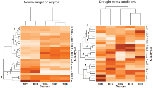
G × E heatmap analysis of cotton seed yield was used to create a visual comparison of year’s effects on the genotypes under the normal irrigation regime and drought stress condition, as well as to determine the range of drought stress responses detectable in these genotypes (Figure 1). The G × E heatmap analysis revealed in two dendrograms in Figure 1: the five years on top and that influenced the distribution of 24 cotton genotypes on the left. The top dendrogram classified the tested environments into two separate clusters in both irrigation conditions. The first cluster (I) consisted of 2019 and 2020, as well as 2020 and 2016 under normal irrigation regime and drought stress conditions, respectively. The second cluster comprises the other years in both irrigation conditions. As for the left dendrogram, 24 genotypes could be classified as six and seven clusters under normal irrigation regime and drought stress condition, respectively. The genotypes within-cluster have the least variance and genetic distance, but the genotypes between clusters are different and have the maximum genetic distance. Except for cluster 1 under normal irrigation conditions, which included G5, G19, and G20 genotypes represented high cotton seed yield across the five environments, there was no clear association between all environments and cotton genotypes. The genotypes in cluster 3 gave the best cotton yield in 2019 and 2020 and low cotton yield in the other years, the opposite was true of cluster 4 under normal irrigation conditions. Based on the heat map under drought stress conditions, the genotypes in cluster 1 (G1, G2, and G6) were among the best performers of cotton yield across most environments, followed by the genotypes in cluster 2. Cluster 4 genotypes (G19, G20, and G24) had the best cotton yield in 2019 and 2018 and moderate to low cotton yield in the other years, but genotype G8 in cluster 3 had the highest cotton yield in 2017 under drought stress conditions. The second and fifth clusters grouped four genotypes (G14, G22, G23, and G10) with the lowest cotton yield across five environments under normal irrigation conditions, similar result by the cluster 5 (G10 and G11) under drought stress conditions. While the other genotypes in the other clusters were intermediate in G × E interactions.

Figure 1. Dendrogram of classified genotypes in growing seasons by cluster analysis during normal irrigation regime and drought stress conditions. The color of each block deepens with the increase of the corresponding cotton seed yield, then the color depth decreases, and the color scale ranges from mild for the moderate yield to white for the lowest yield. The genotypes key names can be found in Table S1. Seasons of 2016, 2017, 2018, 2019, and 2020 represent the five tested environments.

Mean performance and stability of cotton genotypes

Table 5 shows the results of the mean performance and stability parameters based on joint regression and AMMI analysis for 24 cotton genotypes in five environments under normal irrigation regime and drought stress condition. The 24 cotton genotypes revealed significant differences in cotton seed yield under normal irrigation regime and drought stress conditions. The mean cotton seed yield of all genotypes across five environments ranged from 5841.2 to 3674.6 kg ha⁻¹ and from 3655.9 to 2599.8 kg ha⁻¹ under normal irrigation regime and drought stress conditions, respectively. When using mean cotton yield as a first criterion for evaluating the genotypes, several genotypes had means exceeding the grand mean (4515.8 and 3066.9) under normal irrigation regime and drought stress condition, respectively. In general, the genotypes G5 and G19 in both irrigation conditions, the genotypes G20 and G15 in normal irrigation regime and the genotypes G24 and G4 in drought stress conditions gave the better mean cotton yields. While the genotypes G14, G23 and G22, as well as the genotypes G11, G10, and G15 recorded the lowest cotton yields under normal irrigation regime and drought stress conditions, respectively.

Table 5. Mean performance and stability parameters for twenty-four cotton genotypes across environments under normal irrigation regime and drought stress conditions based on joint regression and AMMI analysis.

Genotype code	Normal irrigation regime					Drought stress conditions
	$Y_i$	ASV	$b_i$	$S_{di}^2$	$R_i^2$	$Y_i$	ASV	$b_i$	$S_{di}^2$	$R_i^2$
G1	4394.77	90.38	−1.08**	337617.99**	0.63	3345.84	1.44	1.37^ns	1199958.01**	0.16
G2	4606.66	23.37	0.30**	5629.35^ns	0.42	3136.89	2.37	0.84^ns	1281962.65**	0.06
G3	4860.91	30.46	−0.13**	94431.90^ns	0.06	3182.86	1.19	0.32^ns	254414.62**	0.04
G4	4408.03	31.49	0.37**	−27805.69^ns	0.66	3646.78	1.59	0.21^ns	−14476.94^ns	0.13
G5	5841.16	22.08	−0.05**	111024.71^ns	0.01	3392.09	0.51	1.36^ns	45068.33^ns	0.71
G6	4265.73	20.37	0.86^ns	63914.99^ns	0.77	3144.46	0.97	1.43^ns	257891.24**	0.46
G7	4689.35	43.54	1.93**	−32541.06^ns	0.98	2776.88	2.33	0.58^ns	689281.97**	0.06
G8	4203.47	46.61	0.18**	−36797.70^ns	0.38	2756.24	2.36	0.70^ns	899472.15**	0.06
G9	4624.02	13.08	1.18^ns	−50514.32^ns	0.98	2985.86	0.61	0.25^ns	32685.56^ns	0.09
G10	4075.97	6.86	1.72**	−55609.53^ns	0.99	2677.33	1.93	1.55^ns	216411.02**	0.54
G11	4160.63	13.87	1.07^ns	−63323.30^ns	0.99	2599.81	2.89	1.93^ns	459478.78**	0.49
G12	4498.52	50.62	2.36**	−38001.51^ns	0.99	2718.18	1.31	1.50^ns	19631.23^ns	0.80
G13	4643.59	56.64	2.30**	25145.56^ns	0.97	2783.72	1.09	0.34^ns	375593.99**	0.03
G14	3674.61	65.95	0.27**	−59533.48^ns	0.84	2682.79	0.92	0.82^ns	478087.62**	0.14
G15	4913.91	64.33	2.09**	39997.48^ns	0.96	2651.36	1.56	0.93^ns	715909.89**	0.13
G16	4273.17	12.20	0.94^ns	−53475.86^ns	0.97	3123.75	0.37	1.86^ns	106416.15*	0.74
G17	4490.91	5.36	1.09^ns	−28146.33^ns	0.95	2984.09	2.16	0.96^ns	1090805.32**	0.09
G18	4739.99	44.85	1.89**	−31764.79^ns	0.98	3031.34	2.76	−0.59**	1418682.74**	0.03
G19	5086.3	22.27	0.88^ns	1837.93^ns	0.87	3371.37	3.42	0.47^ns	1292609.18**	0.02
G20	5216.01	29.86	0.92^ns	−51978.83^ns	0.97	3298.95	2.75	0.94^ns	938223.83**	0.10
G21	4277.56	16.23	0.83^ns	−55050.64^ns	0.97	3202.64	0.86	2.72**	−5956.83^ns	0.95
G22	4028.81	3.14	1.51*	26937.10^ns	0.93	3146.57	1.13	2.40**	611735.15**	0.53
G23	4022.58	14.91	1.93**	43957.72^ns	0.95	3312.13	1.63	0.41^ns	240766.58**	0.07
G24	4381.8	20.04	0.63^ns	−63444.85^ns	0.98	3655.88	2.69	0.70^ns	499675.54**	0.10

Superscripted * and ** refer to statistically significant at p ≤0.05 and p ≤0.01, respectively, and ns= non-significant. $Y_i$ = mean cotton seed yield of genotype across environments, ASV = AMMI’s stability value, $b_i$= regression coefficient, $S_{di}^2$= deviation from regression, $R_i^2=$coefficients of determination. The genotypes key names can be found in Table S1.

Joint regression analysis

Most genotypes showed a significant regression coefficient $(b_i)$ and deviation from regression $\left(S_{di}^2\right)$under normal irrigation regime and drought stress condition, respectively, the inverse was true (Table 5). These findings suggest that genotypes already differed in their responses to environmental changes. Some genotypes had $b_i$ close to unity with the highest cotton yield performance (G20 and G19), and with moderate cotton yield performance (G9, G17, G11, G16, G21, and G6). These genotypes also demonstrated specific adaptability to all environments under normal irrigation regimes. Genotypes G2, G14, G15, G17 and G20 with $b_i$ lower than one and close to unity gave the moderate to low cotton yield performance and were adapted to drought stress conditions. G5 ranked first in cotton yield performance with higher $S_{di}^2$, while G24 ranked fifteen in yield with the low $S_{di}^2$ under normal irrigation regimes. As for drought stress conditions, the genotypes G4 and G18 had high and moderate cotton yield performance with the lowest and highest $S_{di}^2$ values and were significantly different from zero, respectively. G4 genotype provided a nice balance of yield and stability. The stability parameter values are the predictability of the estimated response based on Pinthus (1973) coefficients of determination $\left(R_i^2\right)$. Agronomic stability is represented by the $R_i^2$ according to Becker (1981). A genotype with a high coefficient of determination can be considered stable. The $R_i^2$values for the predictability of 24 cotton genotypes for cotton yield show that genotype response explained 1–99% and 2–95% of the mean cotton yield variability across diverse environments normal irrigation regime and drought stress condition, respectively. G21, G12, and G16 have moderate mean cotton yield and higher ${\mathrm{R}}_{\mathrm{i}}^2$, which was the most stable genotypes in both irrigation conditions. While G1 and G18 are highly unstable by JRA statistics under normal irrigation regime and drought stress condition, respectively.

AMMI analysis

The most stable genotypes in both irrigation conditions may be found using the ASV since the PCA1 and PCA2 made up a significant portion of the overall GEI. In proportion to the better option ASV, the genotypes G10, G17, and G22 in normal irrigation regime, the genotype G21 in drought conditions and the genotypes G9 and G16 in both conditions recorded the lowest ASV with moderate to low cotton yield and were stable across environments (Table 5). The ASV ranked the genotypes G1, G15, and G14 in normal irrigation regime and the genotypes G19, G11, G18, and G20 in drought conditions with the highest ASV, as the unstable genotypes with high to moderate yielding performance. Based on the ASV, only G5 had the highest yield across environments and the most stable genotype simultaneously because it had a low ASV value under drought stress conditions.

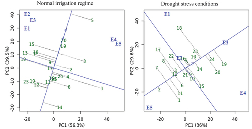
Figure 2 depicts the AMMI biplot of PC1 vs cotton seed yield for 24 cotton genotypes and five environments for cotton seed yield in both conditions. According to Crossa et al. (1990), the genotypes G17, G19, and G20 in normal irrigation regime, the genotypes G23, G5, G12, G4, and G3 in drought conditions and the genotypes G11, G16, G6, G9, and G21 in both conditions had nearly zero scores on the PC1 and least interactive, which indicates that these genotypes were stable, less impacted by the tested environments and suited to all environments. On the other hand, the mean performance of some genotypes was below average. Furthermore, genotypes G5 and G24 exhibited the largest average main effect with the highest PC1 score, indicating that they are more unstable under normal irrigation regime and drought stress condition, respectively. Generally, the genotypes G20 and G5 had lower interaction with high yielding, which makes them relatively stable and the most preferable genotypes under normal and drought conditions, respectively. PC1 scores away from zero lines of biplot indicated that genotypes were adapted to a specific environment, while genotypes with PC1 vectors with the same sign and score but next to zero lines of biplot indicated that genotypes were appropriate to all environments (Murphy et al. 2009; Khan et al. 2021). Some genotypes constructed and located close to the biplot’s origin were the most stable and made the least contribution to GEI, and vice versa (Figure 3). The genotypes G17, G9, G11, G20, G24, and G16 in normal irrigation regime and the genotypes G5, G4, G12, G9, G21, G16, and G3 in drought stress condition are closely from the biplot origin with lower GEI, so they are stable across all environments. While G1 and G18 are unstable since they are further from the origin and contributes more to GEI in normal irrigation regime and drought stress condition, respectively. There is a positive correlation when environment and genotype are positioned close to one another in the biplot, thus specific adaptation (Silveira et al. 2013). For example, the specific adaptation was observed for G1 and G2 with E5 in normal irrigation regime and drought stress condition, respectively.

Figure 2. AMMI biplot of PC1 vs seed yield for twenty-four cotton genotypes (green color) and five environments (blue color) under normal irrigation regime and drought stress conditions. The genotypes and environment key names can be found in Table S1 and Figure S1, respectively.

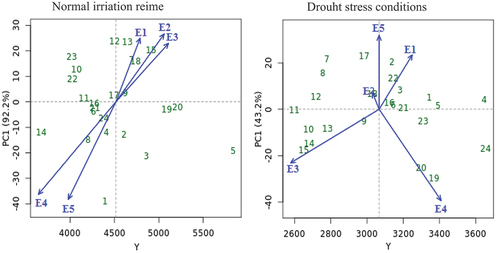
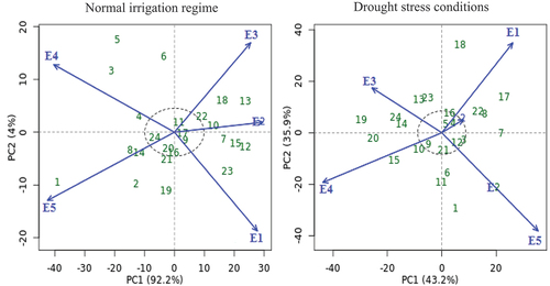
Figure 3. AMMI biplot of PC1 vs PC2 for seed yield with twenty-four cotton genotypes (green color) and five environments (blue color) under normal irrigation regime and drought stress conditions. The genotypes and environment key names can be found in Table S1 and Figure S1, respectively.

GGE biplot analysis

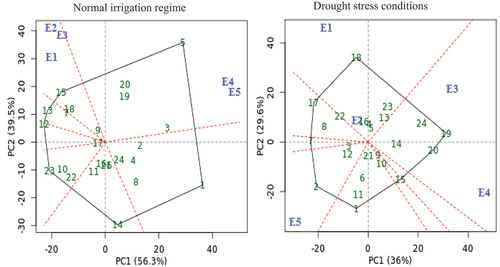
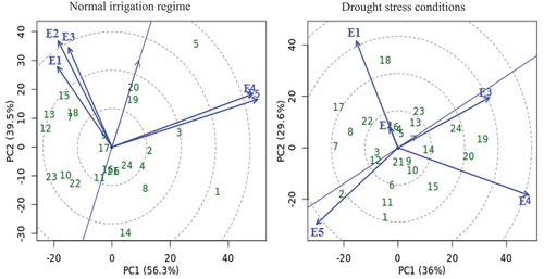
The GGE biplot cotton yield pattern’s polygon view was created to display which genotypes perform best in certain conditions and groupings of environments (Yan et al. 2000), as well as to demonstrate the presence of crossover GEI, mega-environment differentiation, and specific adaptation (Yan and Tinker 2006). Seven (G1, G5, G12, G13, G14, G15, and G23) and eight (G1. G2, G7, G15, G17, G18, G19, and G20) genotypes are located away from the biplot origin in all directions and which formed the polygon vertices during normal irrigation regime and drought stress condition, respectively (Figure 4). While all other genotypes are encompassed within the polygon. A line perpendicular to each polygon side was drawn starting from the biplot origin. The biplot is divided into sectors by these lines. The rays are lines that are perpendicular to the sides of the polygon or their extension (Yan 2002). Thus, the five environments are divided into different apparent groups. The genotype at the vertices of each sector is the nominal highest yielder for the environments or mega-environments that fell into it. Accordingly, G5 produced the best cotton yielding in E4, and E5, while genotype G15 performs best in other environments under normal irrigation conditions. Under the drought stress conditions, G2 was the highest cotton yielder in E5, while G19 was the highest cotton yielder in E3 and E4. The genotypes G24, G22, and G23 were under normal irrigation regimes, and the genotypes G10, G11, and G15 were the poorest across the tested environments, due to no environment falling into the sectors of these genotypes.

Figure 4. GGE biplot polygon of ‘which-won-where’ for seed yield with twenty-four cotton genotypes (green color) and five environments (blue color) under normal irrigation regime and drought stress conditions. The genotypes and environment key names can be found in Table S1 and Figure S1, respectively.

To assess genotype yield stability using average PCAs in all environments, the average environment coordination (AEC) method was utilized based on genotype-focused singular value partitioning (SVP). If SVP = 1, the AEC line with a single arrow passes through the biplot’s origin (Yan 2002), the arrow points to a higher mean yield. The meaning of PC1 and PC2 of the environmental scores is defined, as a report by Yan and Rajcan (2002). The ‘Mean vs. stability’ view is frequently referred to as AEC with SVP = 1 which helps to simplify the genotype assessment based on the mean performance and stability across environments within a mega-environment (Figure 5). The GGE biplot was created by plotting the PC1 and PC2 produced from subjecting data of environment-centered yield to singular value decomposition (Yan et al. 2000). The genotypes are grouped according to their average cotton yielding, as indicated by the arrow sign on the AEC. The genotypes with above-average means were from G5 to G2 and from G19 to G9, while those with below-average means were from G12 to G14 and from G10 to G2 in normal irrigation regime and drought stress condition, respectively. Genotype G5, G20 and G19 produced higher cotton yield in E4 and E5 in normal irrigation regime, while the low yield was recorded by G23 in the same environments. As for during drought conditions, G24, G19 and G20 had the highest mean cotton yield, whereas G11 had the least mean cotton yield in E3 and E4. The highest cotton yield was recorded for genotype G1 and G2 in E5 under normal irrigation regime and drought stress conditions, respectively. G11, G16, G17, G19, G20, and G21 in normal and G12, G2, G3, G5, G13, and G21 in drought conditions were the most stable genotypes, as they were located almost on the AEC abscissa and had a near-zero projection onto the AEC ordinate. According to Yan et al. (2007), this shows that these genotypic rankings were highly consistent across environments. In addition to good cotton yield, genotype stability is more important, in terms of Yan (2001) defined an ‘ideal’ genotype based on mean performance as well as stability. Thus, the genotypes G20 and G19 in normal irrigation conditions and the genotypes G5 and G4 in drought conditions are more stable with better mean cotton yield than other genotypes. Conversely, the genotypes G1 and G18 are more variable and highly unstable with below- and above-average mean performance in both conditions, respectively.

Figure 5. GGE biplot of mean vs. stability for seed yield with twenty-four cotton genotypes (green color) and five environments (blue color) under normal irrigation regime and drought stress conditions. The genotypes and environment key names can be found in Table S1 and Figure S1, respectively.

Evaluation of the test environments

For a successful breeding approach in the selection of superior genotypes for a mega-environment, determining the best-suited (ideal) test environment is critical by the test-environment evaluation (Yan et al. 2007).

AMMI analysis

The long vectors and highest cotton yield were observed for E3 and E4 environments under normal irrigation regime and drought stress condition, respectively (Figures 2 and 3), indicating these environments have an important influence on the GEI determination. The test environments E1, E2, and E3 had the highest PC1 and lowest PC2 scores with the highest yielding performance, based on environmental PCAs scores in normal irrigation regimes. As for drought conditions, the highest PC1 and lowest PC2 scores with the higher cotton productivity were recorded by the E1 and E2. Thus, these environments can be considered ideal test environments, while the opposite was true of the other environments. In AMMI biplot, short vectors closer to zero and close to biplot origin were observed for E1, E2, and E3 in normal irrigation regime and E2 and E1 in drought stress condition, thus these environments are less interlining and most stable that nearly guarantee all genotypes in that environment to perform better. Also, the angles between these environments are below 90.

GGE biplot

The idealness of the tested environments is defined by two characteristics: a) discrimitiveness (the ability of an environment to differentiate genotype in terms of main genotype effects), which has a high PC1 score, and b) representativeness (the ability of an environment to represent all other evaluated environments), which has a zero score for PC2. As a report by Yan et al. (2007), due to having the smallest angles with AEC, the test environment E3 in both irrigation conditions are more representative of other test environments (Figure 6), indicating that this environment is idyllic and has the greatest ability to discriminate genotypes, thus favoring the selection of superior genotypes. Yan et al. (2000) and Yan and Rajcan (2002) reported that the most genotypes desirable are the one closest to the graph of the ideal environment. Thus, the genotype G5 is the most productive and stable in both irrigation conditions. While the test environment E5 had a larger angle with AEC, indicating that it was the least discriminating and representative in both irrigation conditions. Non-discriminating test environments provide minimal information about genotypes and must not be used as test environments (Yan and Tinker 2006). According to Yan and Kang (2002), the acute angles (strong positive correlation) were observed among E1, E2 and E3 and between E4 and E5 in normal irrigation conditions, while E3 had positively correlated with E2, E4 (moderate) and E1 (slight) in drought stress conditions (Figure 6). As a report by Yan and Tinker (2006), the length vectors and the cosine of the angle between the two environments determine the similarity (covariance) of them. Therefore, the environments in normal irrigation conditions were divided into two distinct groups by the ray lines: the first group included E4 and E5, and the second group comprised the other environments. As for drought stress conditions, there are three groups: the first group consists of E3 and E4, the second group is composed of E1 and E2, while E5 belongs to the third group.

Figure 6. GGE biplot of discrimitiveness vs. representativeness for seed yield with twenty-four cotton genotypes (green color) and five environments (blue color) under normal irrigation regime and drought stress conditions. The genotypes and environment key names can be found in Table S1 and Figure S1, respectively.

Relationships between JRA, AMMI, and GGE biplot models

According to the ranks of 24 genotypes in five environments (Table 6), the stability statistics based on JRA, AMMI and GGE models identified G11, G20 and G16 in normal irrigation conditions and G5, G21 and G12 in drought as the most stable genotypes, while G1 and G18 as unstable ones in normal irrigation regime and drought stress condition, respectively. The other genotypes fell somewhere in the middle of these two groupings. Spearman correlation coefficients for each pair of cotton yield and stability statistics based on JRA, AMMI and GGE models are shown in Table 7. Mean yield of cotton seed was not significantly correlated with JRA, AMMI and GGE models in both irrigation conditions, but it was low correlated positively with the GGE model in drought stress conditions. During the stability analysis of both irrigation conditions, $b_i$, $S_{di}^2$ (JRA model), ASV (AMMI model) and GGE biplot were positively and significantly correlated (p ≤0.05 or 0.01) with each other in their ranking of the genotypes, except ASV with $S_{di}^2$, and $b_i$ with ASV and GGE in normal irrigation regime and drought stress condition, respectively. $S_{di}^2$ with $b_i$ and $R_i^2$ in normal irrigation regime and $R_i^2$ with ASV and $S_{di}^2$ in drought stress condition were positively and significantly correlated (p ≤0.05 or 0.01) in the ranking of genotypes for stability analysis

Table 6. Ranks of twenty-four genotypes in five environments using mean cotton yield stability statistics based on JRA, AMMI and GGE models.

Genotype code	Normal irrigation regime						Drought stress conditions
	$Y_i$	ASV	GGE	$b_i$	$S_{di}^2$	$R_i^2$	$Y_i$	ASV	GGE	$b_i$	$S_{di}^2$	$R_i^2$
G1	14	24	24	24	24	20	5	11	21	9	21	9
G2	10	13	13	12	16	21	12	19	2	4	22	18
G3	5	15	20	21	22	23	9	9	3	17	9	21
G4	13	16	11	11	14	19	2	13	9	19	1	11
G5	1	11	19	19	23	24	3	2	4	8	5	4
G6	18	10	8	6	21	18	11	6	14	11	10	8
G7	7	17	17	18	11	4	18	17	15	10	16	18
G8	19	19	15	15	10	22	19	18	18	7	18	18
G9	9	5	7	8	8	4	15	3	8	18	4	15
G10	21	3	12	13	4	1	22	15	13	14	7	5
G11	20	6	3	2	2	1	24	23	16	21	12	7
G12	11	20	23	23	9	1	20	10	1	12	3	2
G13	8	21	22	22	17	8	17	7	5	16	11	22
G14	24	23	14	14	3	17	21	5	10	5	13	10
G15	4	22	21	20	19	12	23	12	22	3	17	11
G16	17	4	1	1	6	8	13	1	12	20	6	3
G17	12	2	6	4	13	13	16	16	23	1	20	15
G18	6	18	16	16	12	4	14	22	24	23	24	22
G19	3	12	5	5	15	16	4	24	17	13	23	24
G20	2	14	2	3	7	8	7	21	20	2	19	13
G21	16	8	4	7	5	8	8	4	6	24	2	1
G22	22	1	10	10	18	15	10	8	19	22	15	6
G23	23	7	18	17	20	13	6	14	11	15	8	17
G24	15	9	9	9	1	4	1	20	7	6	14	13

$Y_i$ = mean cotton seed yield of genotype across environments, ASV = AMMI’s stability value, $b_i$= regression coefficient, $S_{di}^2$= deviation from regression, $R_i^2=$coefficients of determination. The genotypes key names can be found in Table S1.

Table 7. Spearman’s rank correlation coefficients among mean cotton yield and stability statistics of different statistical models across normal irrigation regime and drought stress conditions.

Stability statistics	Normal irrigation regime					Drought stress conditions
	$Y_i$	ASV	GGE	$b_i$	$S_{di}^2$	Yi	ASV	GGE	$b_i$	$S_{di}^2$
ASV	−0.32					0.02
GGE	−0.19	0.67**				0.17	0.42*
$b_i$	−0.21	0.67**	0.99**			−0.06	−0.23	−0.13
$S_{di}^2$	−0.33	0.23	0.55*	0.50*		0.05	0.65**	0.64**	−0.44*
$R_i^2$	−0.10	0.24	0.23	0.20	0.67**	−0.07	0.51*	0.16	−0.16	0.57**

$Y_i$ = mean cotton seed yield of genotype across environments, ASV = AMMI’s stability value, $b_i$= regression coefficient, $S_{di}^2$= deviation from regression, $R_i^2=$coefficients of determination. Superscripted * and ** refer to statistically significant at p ≤0.05 and p ≤0.01, respectively.

Discussion

Results of combined ANOVA, Eberhart and Russel JRA as well AMMI analysis showed significant differences among genotypes (G), environments (E), and their interactions (GEI) for cotton seed yield in both irrigation conditions. These results indicate the existence of high diversity among genotypes and confirm that the testing environments were different, which enables us to select genotypes under both irrigation conditions, especially drought stress. Also, our results indicated the variability and inconsistency in the cotton seed yield in responses of 24 genotypes over the five environments in both irrigation conditions, as determined by these models. So, assessing the stability of cotton seed yield for these different genotypes, especially under drought stress conditions, would be perfect for selecting a cotton genotype with higher cotton seed yield and better stability. Interestingly, the above trends are like those that were reported in earlier studies on cotton used combined ANOVA (Killi and Harem 2006; Mudada et al. 2017), Eberhart and Russel JRA model (Kumbhalkar et al. 2021; Vavdiya et al. 2021) and AMMI model (Riaz et al. 2019; Teodoro et al. 2019; Lingaiah et al. 2020). Moreover, the combined ANOVA, JRA and AMMI models allow hypothesis testing, while the GGE biplot approach lacks a serious statistical test (Ding et al. 2008).

The significance of the GEI as a source but does not analyze it can be tested using ANOVA, although this test may be misleading (Zobel et al. 1988). According to Moll et al. (1978), a significant GEI can be partitioned into components representing genotypic differences in responsiveness to environmental variation and differences in correlations between pairs of genotypes under environments evaluated. The GEI was partitioned by JRA, AMMI and GGE biplot, but the AMMI model partitioned the SS of GEI more effectively than them. The SS% of GEI contained in JRA (93%) was close to the AMMI model and GGE biplot (96%) under normal irrigation conditions. While it was higher in the AMMI model (79%) than in GGE biplot (66%) and JRA (25%) under drought stress conditions. These findings show the superiority of the AMMI model and accounted for more GEI variation in cotton yield, followed by GGE biplot over the regression model under drought stress conditions. A similar trend has been reported in cotton under water-deficit conditions by Riaz et al. (2019). The AMMI model was superior because it can analyze the GEI data more than ANOVA and JRA (Zobel et al. 1988), JRA (Aremu et al. 2006), and JRA and GGE biplot (Kumar et al. 2016; Alizadeh et al. 2017). The ANOVA and JRA are all subcases of the more comprehensive and complete AMMI model, thus the AMMI model offers a more appropriate first statistical analysis of yield trials that may have a GEI (Zobel et al. 1988). While the GGE biplot always explains more variation of GEI compared to the AMMI model, according to Yan et al. (2007). According to Kendal and Tekdal (2016), the AMMI model showed evidence of the GEI, particularly when the interaction was split between two PCAs. The GEI model based on AMMI analysis proved that the genotypes can be considered as a candidate, due to extensive adaptability and strong performance in all environments (Tekdal and Kendal 2018).

Cotton productivity was shown to be significantly lower under drought stress conditions than under normal irrigation regimes and ranged from 9.03% by G24 and 29.91% by G15 across five environments, suggesting genetic variability in 24 cotton genotypes for drought tolerance. Bakhsh et al. (2019) and Mahmood et al. (2021) both reported similar findings. G × E heatmap analysis of cotton seed yield classified the genotypes and environments into different separate clusters in both irrigation conditions. Generally, the genotypes G5, G19, and G20 had the maximum cotton yield across all environments, according to the heatmap of normal irrigation regime and drought stress condition, while the genotypes G10, G11, and G14 had the lowest cotton yield. During the normal irrigation regime, these genotypes gave the best seed yielding, but some genotypes also performed well under drought stress conditions (G1, G4 and G24), indicating their inconsistent relative performance and high sensitivity to environmental variation (El-Hashash and Agwa 2018). Thillainathan and Fernandez (2002) stated that yield stability may be due to consistent performances across different environments (sites and/or years). The GEI effect was of the crossover type, as evidenced by the differential yield ranking of genotypes across environments (Yan and Hunt 2001).

The understanding of contributions of genotypes, environments, and their interactions as sources of variation could potentially aid for the breeders in developing more stable genotypes (Basford and Cooper 1998). The fact that there was a significant GEI for yield shows that some genotypes were stable while others were unstable (El-Hashash and Agwa 2018). Only qualitative or crossover interactions are relevant in agriculture, according to Baker (1988) and Crossa (1990), and suitable statistical analysis is necessary to quantify them. Therefore, there is a need for assessing the stability of yield for each of the 24 cotton genotypes to identify genotypes with superior cotton yield under drought stress conditions by applying either JRA, AMMI or GGE biplot models.

Most cotton genotypes tested in this study were high-yielding and stable due to it having non-significant JRA parameters, as reported by Kumbhalkar et al. (2021) and Vavdiya et al. (2021). AMMI-ASV parameter is a suitable stability index in discriminating stable genotypes with high mean yield performance in cotton (Gibely and Hassan 2018) and in common bean across drought environments (Burbano-Erazo et al. 2021). Generally, the three models JRA, AMMI and GGE biplot were similar in ranking genotypes for stability across environments. Alizadeh et al. (2017) mentioned that although the variation described by the three models differed, they all produced similar results of genotypes ranking. The three models identified G20 and G5 as stable genotypes with the highest mean cotton seed yield across environments under normal irrigation regime and drought stress conditions, respectively. While G1 and G18 were the unstable genotypes under normal irrigation regime and drought stress condition, respectively. The interpretations of biplot graphics are the most reliable for representing standards in applied data (Machado et al. 2019). In the investigation of GEI, both AMMI model and GGE biplot were effectively provided favorable findings; however, the GGE biplot was the most efficient since it showed a clear distinction among evaluated genotypes in terms of yields and stability across normal irrigation regime and drought stress condition. It appears that a combination of parametric and non-parametric stability statistics can be utilized as an extra tool to allow better decisions aid in the selection of superior genotypes (Pour-Aboughadareh et al. 2022).

Site selection in the multi-environment trials is influenced by the ideal environment, which is simply an approximation (Tena et al. 2019). Thus, the AMMI model and GGE biplot can also be compared in terms of their ability to identify appropriate test locations in multi-environment trials (Alizadeh et al. 2017). According to the AMMI biplot and the GGE biplot, test environments E2 and E3 for cotton seed yield are regarded as the ideal environments under normal irrigation regime and drought stress condition, respectively. These environments tend to discriminate the genotypes in the same direction (Alizadeh et al. 2017), and they are used as an excellent index for selecting genotypes with the best average performance and adaptability (Murphy et al. 2009). Oppositely, test environment E5 was found to be the worst environment for genotype selection in both irrigation conditions. The ideal test environment would be appropriate for selecting superior genotypes due to its high discriminating power and representativeness. GGE biplot can visually rank test environments for their usefulness in identifying superior genotypes based on the distances between their markers and the marker of the ideal test environment (Yan et al. 2007). In cotton, large environmental groups were formed based on the environmental conditions using the GGE biplot (Yaşar 2023). While AMMI biplot (Zobel et al. 1988) provides no information on the environment’s ability to identify superior genotypes (Yan et al. 2007), thus an ideal environment for selecting superior genotypes could not be visualized in AMMI biplot (Alizadeh et al. 2017). The GGE biplot is more repeatable if it is calculated within mega-environments because the mean yield is more repeatable (Pour-Aboughadareh et al. 2022). In cotton, the GGE biplot is a simple approach to assess the effect of genotype on the environment, and it gives useful information about the genotypes and environments under study (Kamali et al. 2015; Sadabadi et al. 2018). Additionally, Shahriari et al. (2018) stated that the distribution of genotypes for the traits examined in both AMMI graphs and GGE biplots showed that genotypes originated from locations with similar environmental conditions that were situated adjacent to one another.

The stability statistics based on JRA, AMMI and GGE models fell within the static or biological stability concept because they are not correlated with cotton seed yield in their ranking of the genotypes across both irrigation conditions. These results suggest that the stability parameters provide information that cannot be gleaned from average yield alone (Mekbib 2002). The stability of these models represents the concept of static or biological stability, which was influenced simultaneously by both yield and stability. To maximize the benefits of GEI and make genotype selection more exact and refined, both yield and stability of performance should be examined simultaneously (El-Hashash et al. 2019). As a result, these parameters can be used to identify genotypes that are adapted to harsh growth conditions and as compromise techniques for selecting genotypes with a moderate yield and good stability (El-Hashash and Agwa 2018). AMMI-based stability measures such as ASV exhibited a positive and significant correlation with mean yield, according to Ajay et al. (2018), indicating that it has a dynamic concept of stability. The significant positive correlation among JRA, AMMI and GGE models indicate their similar information about ranking genotypes for stability across environments. Therefore, any parameter of them or interchangeably can be used to select high-yielding and stable genotypes. Similar findings were mentioned by Alizadeh et al. (2017). In comparison to JRA and AMMI models, the GGE biplot model combines some of the characteristics of all of them and allows for a visual interpretation of GEI (Ding et al. 2008). Also, Alizadeh et al. (2017) added that the GGE biplot was more versatile and flexible compared to the JRA and AMMI models, and it provided a better understanding of GEI.

The GGE biplot is superior to the AMMI graph in the mega-environment analysis and genotype evaluation in several things, which are as follows: genotype evaluation by mean vs. stability view, explains more G+GE, easier to visualize the which-won-where patterns (AMMI could be misleading), has the inner-product property of the biplot, effective in evaluating test environments by discriminating power vs. representativeness (which is not possible in AMMI analysis) and shows the relative performance of each genotype in each environment (Yan 2006). As for the mega-environment delineation and winning genotypes, Hassani et al. (2018) revealed that the results of the AMMI model were partially in agreement with the results of the GGE biplot analysis. Furthermore, the GGE biplot is more rational and biological for practice than AMMI analysis in terms of explaining the PC1 score, which shows the genotypic effect rather than the additive main effect (Yan et al. 2000). Generally, the GGE biplot is always close to the best AMMI models in most cases, when compared to different AMMI family models (Ma et al. 2004). The best genotypes for all traits in crops can be found using the genotype × yield trait biplot approach (Kendal 2019). Finally, the JRA, AMMI, and GGE biplot models determined that genotype G5 and G20 were the most biologically stable with the high cotton seed yield and are recommended for cultivation under environments with different moisture regimes and poor climatic conditions. Furthermore, these methods compared were conformable in the identification of the promising Egyptian cotton cultivars with high performance and higher yield stability across normal irrigation regime and drought stress condition.

Conclusions

The results of the combined ANOVA, JRA, and AMMI models reflect the divergent climatic conditions of the five environments, resulting in a high level of genetic variability among 24 genotypes for cotton seed yield in both irrigation conditions. The combined ANOVA, JRA and AMMI models allow hypothesis testing, while the GGE biplot approach lacks a serious statistical test. The AMMI model was superior because it can analyze the GEI data more than JRA and GGE biplot under drought stress conditions. The JRA, AMMI and GGE biplot models showed similarity and effectiveness in ranking and detecting stable genotypes over environments in both irrigation conditions. In contrast to the JRA model, the models of AMMI and GGE biplot performed well in the study of the GEI and provided a clear idea of genotype stability behavior in both irrigation conditions. The AMMI and GGE biplot models produced acceptable results; however, the GGE biplot model was the most efficient and appropriate for polygon view, better visualization of biplot and evaluating test environments. The three methods compared were concordant in their ability to separate, rank, and identify the promising G5 and G20 genotypes with higher yield stability and high drought-tolerant in regions with limited irrigation-water across different mega-environments. Furthermore, the methods studied were conformable in the identification of the promising cotton cultivars with high mean performance and higher yield stability across different environments and soil moisture regimes.

Disclosure statement

No potential conflict of interest was reported by the author(s).

Supplemental data

Supplemental data for this article can be accessed online at https://doi.org/10.1080/03650340.2023.2287759

Additional information

Funding

This work was supported by the Cotton Research Institute, Agriculture Research Center, Giza, Egypt.

References

- Acciaresi HA, Chidichimo HO, Fuse CB. 1997. Study of genotype x environment interaction for forage yield in oat (Avena sativa L.) with joint linear regression analysis and AMMI analysis. Cereal Res Commun. 25(1):55–62. doi: 10.1007/BF03543884.
- Ahmed YN, Delin H. 2019. Current situation of Egyptian cotton: econometrics study using ARDL model. J Agric Sci. 11(10):88–97.. doi: 10.5539/jas.v11n10p88.
- Ajay BC, Aravind J, Abdul Fiyaz R, Bera SK, Narendrakumar Gangadhar K, Kona P. 2018. Modified AMMI stability index (MASI) for stability analysis. Groundn Newsl. 18:4–5.
- Alizadeh K, Mohammadi R, Shariati A, Eskandari M. 2017. Comparative analysis of statistical models for evaluating genotype × environment interaction in rainfed safflower. Agric Res. 6(4):455–465. doi: 10.1007/s40003-017-0279-1.
- Allard RW, Bradshaw AD. 1964. Implication of genotype environmental interactions in plant breeding. Crop Sci. 4(5):503–508. doi: 10.2135/cropsci1964.0011183X000400050021x.
- Allen RG, Pereira LS, Raes D, Smith M 1998. Crop evapotranspiration-guidelines for Computing Crop water requirements-FAO irrigation and drainage paper 56. FAO, p. 56, Rome, Italy
- Alwala S, Kwolek T, McPherson M, Pellow J, Meyer D. 2010. A comprehensive comparison between Eberhart and Russell joint regression and GGE biplot analyses to identify stable and high yielding maize hybrids. Field Crops Res. 119(2–3):225–230. doi: 10.1016/j.fcr.2010.07.010.
- Annicchiarico P. 1997. Joint regression vs AMMI analysis of genotype-environment interactions for cereals in Italy. Euphytica. 94(1):53–62. doi: 10.1023/A:1002954824178.
- Aremu C, Ojo DK, Oduwaye OA, Amira J. 2006. Comparison of joint regression analysis (JRA) and additional main effect and multiplicative interaction (AMMI) model in the study of g x e interaction in soybean across two agroecological zones in Nigeria. Niger J Genet. 20(1):74–83. doi: 10.4314/njg.v20i1.42256.
- Baker RJ. 1988. Tests for crossover genotype-environment interactions. Can J Plant Sci. 68(2):405–410. doi: 10.4141/cjps88-051.
- Bakhsh A, Rehman M, Salman S, Ullah R. 2019. Evaluation of cotton genotypes for seed cotton yield and fiber quality traits under water stress and non-stress conditions. Sarhad J Agric. 35(1):161–170. doi: 10.17582/journal.sja/2019/35.1.161.170.
- Basford KE, Cooper M. 1998. Genotype × environmental interactions and some considerations of their implications for wheat breeding in Australia. Aust J Agric Res. 49(2):153–174. doi: 10.1071/A97035.
- Bowman JC. 1972. Genotype × environment interactions. Genet Sel Evol. 4(1):117. doi: 10.1186/1297-9686-4-1-117.
- Brouwer C, Heibloem M. 1986. Irrigation water management: irrigation water needs. Training manual. Rome: FAO. https://ftp.fao.org/agl/aglw/fwm/Manual3.pdf
- Burbano-Erazo E, León-Pacheco RI, Cordero-Cordero CC, López Hernández F, Cortés AJ, Tofiño-Rivera AP. 2021. Multienvironment yield components in advanced common bean (phaseolus vulgaris L.) tepary bean (P. acutifolius A. Gray) interspecific lines for heat and drought tolerance. Agronomy. 11(10):1978. doi: 10.3390/agronomy11101978.
- Clarke JM, De Pauw RM, Townley-Smith TM. 1992. Evaluation of methods for quantification of drought tolerance in wheat. Crop Sci. 32(3):728–732. doi: 10.2135/cropsci1992.0011183X003200030029x.
- Crossa J. 1990. Statistical analysis of multilocation trials. Adv Agron. 44:55–86. doi: 10.1016/S0065-2113:60818-4.
- Crossa J, Gauch HG, Zobel RW. 1990. Additional main effects and multiplicative interaction analysis of two international maize cultivar trials. Crop Sci. 30(3):493–500. doi: 10.2135/cropsci1990.0011183X003000030003x.
- Ding M, Tier B, Yan W, Wu HX, Powell MB, TA M. 2008. Application of GGE biplot analysis to evaluate genotype (G), environment (E) and G × E interaction on P. radiata: a case study. New Zealand J Forest Sci. 38(1):132–142.
- Ebdon JS, Gauch HG. 2002. Additional main effects and multiplicative interaction analysis of national turfgrass performance trials. Crop Sci. 42(2):497–506. doi: 10.2135/cropsci2002.4970.
- Ebem EC, Afuape SO, Chukwu SC, Ubi BE. 2021. Genotype × environment interaction and stability analysis for root yield in sweet potato [ipomoea batatas (L.) lam]. Front Agron. 3:665564. doi: 10.3389/fagro.2021.665564.
- Eberhart SA, Russell WA. 1966. Stability parameters for Comparing Varieties 1. Crop Sci. 6(1):36–40. doi: 10.2135/cropsci1966.0011183X000600010011x.
- El-Hashash EF, Abou El-Enin MM, Abd El-Mageed TA, Attia MAEH, El-Saadony MT, El-Tarabily KA, Shaaban A. 2022. Bread wheat productivity in response to humic acid supply and supplementary irrigation mode in three Northwestern coastal sites of Egypt. Agronomy. 12(7):1499. doi: 10.3390/agronomy12071499.
- El-Hashash EF, Agwa AM. 2018. Comparison of parametric stability statistics for grain yield in barley under different drought stress severities. Merit Res J Agric Sci Soil Sci. 6(7):098–111.
- El-Hashash EF, Hassan AE, Agwa AM. 2018. Genotype by environment interaction effects and evaluation of drought tolerance indices under normal and severe stress conditions in barley. Int J Plant Breed Crop Sci. 5(2):300–316.
- El-Hashash EF, Tarek SM, Rehab AA, Tharwat MA. 2019. Comparison of non-parametric stability statistics for selecting stable and adapted soybean genotypes under different environments. Asian J Res Crop Sci. 4(4):1–16. doi: 10.9734/ajrcs/2019/v4i430080.
- El Sherbiny HA, El-Hashash EF, El-Enin MM A, Nofal RS, El-Mageed TA A, Bleih EM, El-Saadony MT, El-Tarabily KA, Shaaban A. 2022. Exogenously applied salicylic acid boosts morpho-physiological traits, yield, and water productivity of lowland rice under normal and deficit irrigation. Agronomy. 12(8):1860. doi: 10.3390/agronomy12081860.
- Falconer DS, Mackay TFC. 1996. Introduction to quantitative genetics. 4th ed. New York: Longman; pp. 132–133.
- Finlay KW, Wilkinson GN. 1963. Analysis of adaptation in a plant breeding programme. Aust J Agric Res. 14(6):742–754. doi: 10.1071/AR9630742.
- Gauch HG. 2013. A simple protocol for AMMI analysis of yield trials. Crop Sci. 53(5):1860–1869. doi: 10.2135/cropsci2013.04.0241.
- Gauch HG, Piepho HP, Annicchiarico P. 2008. Statistical analysis of yield trials by AMMI and GGE: further considerations. Crop Sci. 48(3):866–889. doi: 10.2135/cropsci2007.09.0513.
- Gauch HG, Zobel RW. 1996. AMMI analysis of yield trials. In: Kang M Gausch H, editors Genotype-by environment interaction. Boca Raton (FL): CRC Press; pp. 85–122.
- Gauch HG, Zobel RW. 1997. Identifying mega-environment and targeting genotypes. Crop Sci. 37(2):381–385. doi: 10.2135/cropsci1997.0011183X003700020002x.
- Ghaed-Rahimi L, Heidari B, Dadkhodaie A. 2014. Genotype × environment interactions for wheat grain yield and antioxidant changes in association with drought stress. Arch Agron Soil Sci. 61(2):153–171. doi: 10.1080/03650340.2014.926004.
- Gibely R, Hassan S. 2018. Estimating of stability parameters among some extra-long staple cotton genotypes under different environments. Journal Of Plant Production. 9(5):459–468. doi: 10.21608/jpp.2018.35805.
- Hall AE. 1993. Is dehydration tolerance relevant to genotypic differences in leaf senescence and crop adaptation to dry environments? In: Close TJ, and Bray EA, editors. Plant responses to cellular dehydration during environmental stress. California: Academic; pp. 1–10.
- Hassani M, Heidari B, Dadkhodaie A, Stevanato P. 2018. Genotype by environment interaction components underlying variations in root, sugar and white sugar yield in sugar beet (beta vulgaris L.). Euphytica. 214(4):79. doi: 10.1007/s10681-018-2160-0.
- Israelsen OW, Hansen VC. 1962. Irrigation principles and practices. New York, U.S.A: John Wiley & Sons Inco.
- Kamali A, Fakheri BA, Zabet M. 2015. The study of drought stress effects on yield and yield components of cotton using biplot analysis. Iranian J Cotton Res. 3(5):33–47. doi: 10.22092/IJCR.2016.106074.
- Kang MS. 1998. Using genotype-by-environment interaction for crop cultivar development. Adv Agron. 62:199–252. doi: 10.1016/S0065-2113(08)60569-6.
- Kendal E. 2019. Comparing durum wheat cultivars by genotype × yield × trait and genotype × trait biplot method. Chil J Agric Res. 79(4):512–522. doi: 10.4067/S0718-58392019000400512.
- Kendal E, Tekdal S. 2016. Application of AMMI model for evaluation spring barley genotypes in multi-environment trials. Bangladesh J Bot. 45(3):613–620.
- Khan MMH, Rafii MY, Ramlee SI, Jusoh M, Al Mamun MD. 2021. AMMI and GGE biplot analysis for yield performance and stability assessment of selected Bambara groundnut (Vigna subterranea L. Verdc.) genotypes under the multi-environmental trials (METs). Sci Rep. 11(1):22791. doi: 10.1038/s41598-021-01411-2.
- Killi F, Harem E. 2006. Genotype × environment interaction and stability analysis of cotton yield in Aegean region of Turkey. J Environ Biol. 37(2):427–430.
- Klute A, Dirksen C. 1986. Methods of soil analysis: physical and mineralogical methods. Madison (WI): ASA and SSSA Chapter 28, Hydraulic Conductivity And Diffusivity. Lab Method. 687–734. doi: 10.2136/sssabookser5.1.2ed.c28.
- Kroonenberg PM. 1995. Introduction to biplots for G×E tables. Brisbane: University of Queensland.
- Kumar V, Kharub AS, Verma RPS, Verma A. 2016. AMMI, GGE biplots and regression analysis to comprehend the G × E interaction in multi-environment barley trials. Indian J Genet. 76(2):202–204. doi: 10.5958/0975-6906.2016.00033.X.
- Kumbhalkar HB, Gawande VL, Deshmukh SB, Gotmare V, Waghmare VN. 2021. Genotype x environment interaction for seed cotton yield and component traits in upland cotton (gossypium hirsutum L.). Electron J Plant Breed. 12(4):1209–1217. doi: 10.37992/2021.1204.166.
- Levene H. 1960. Robust tests of equality of variances. In: Olkin I, Ghurye SG, Hoeffding W, Madow WG Mann HB, editors Contributions to probability and statistics, essays in honor of Harold Hoteling. Stanford, CA, USA: Stanford University Press; pp. 278–292.
- Lingaiah N, Sudharshanam A, Rao VT, Prashant Y, Kumar MV, Reddy PI, Prasad BR, Reddy PRR, Rao PJM. 2020. AMMI biplot analysis in cotton (gossypium hirsutum L.) genotypes for genotype × environment interaction at four agro-ecologies in Telangana state. Current J Applied Sci Technol. 39(15):98–103. doi: 10.9734/cjast/2020/v39i1530722.
- Machado NG, Lotufo-Neto N, Hongyu K. 2019. Statistical analysis for genotype stability and adaptability in maize yield based on environment and genotype interaction models. Ciência E Natura. 41(e25):1–9. doi: 10.5902/2179460X32873.
- Mahmood T, Wang X, Ahmar S, Abdullah M, Iqbal MS, Rana RM, Yasir M, Khalid S, Javed T, Mora-Poblete F, et al. 2021. Genetic potential and inheritance pattern of phenological growth and drought tolerance in cotton (Gossypium hirsutum L.). Front Plant Sci. 12:705392. doi: 10.3389/fpls.2021.705392.
- Ma B, Yan W, Dwyer LM, Frégeau-Reid JA, Voldeng HD, Dion Y, Nass HG. 2004. Graphic analysis of genotype, environment, nitrogen fertilizer, and their interactions on spring wheat yield. Agron J. 96(1):169–180. doi: 10.2134/agronj2004.1690.
- McKeand SE, Li B, Hatcher AV, Weir RJ. 1990. Stability parameter estimates for stem volume for loblolly pine families growing in different regions in the southeastern United States. Front Sci. 36(1):10–17. doi: 10.1093/forestscience/36.1.10.
- Mekbib F. 2002. Simultaneous selection for high yield and stability in common bean (Phaseolus vulgaris) genotypes. J Agric Sci. 138(3):249–253. doi: 10.1017/S0021859602001946.
- Mekdad AAA, Ahmed MAE, Mostafa MR, Ahmed S. 2021b. Culture management and application of humic acid in favor of Helianthus annuus L. oil yield and nutritional homeostasis in a dry environment. J Soil Sci Plant Nutr. 22(1):71–86. doi: 10.1007/s42729-021-00636-4.
- Mekdad AA, El-Enin MMA, Rady MM, Hassan FA, Ali EF, Shaaban A. 2021a. Impact of level of nitrogen fertilization and critical period for weed control in peanut (Arachis hypogaea L.). Agronomy. 11(5):909. doi: 10.3390/agronomy11050909.
- Mohammadi R, Amri A. 2008. Comparison of parametric and non-parametric methods for selecting stable and adapted durum wheat genotypes in variable environments. Euphytica. 159(3):419–432. doi: 10.1007/s10681-007-9600-6.
- Moll RH, Cockerham CC, Stuber CW, Williams WP. 1978. Selection responses, genetic-environmental interactions, and Heterosis with recurrent selection for yield in maize 1. Crop Sci. 18(4):641–645. doi: 10.2135/cropsci1978.0011183X001800040029x.
- Mudada N, Chitamba J, Macheke TO, Manjeru P. 2017. Genotype × environmental interaction on seed cotton yield and yield components. Open Access Library J. 4(11):1–22. doi: 10.4236/oalib.1103192.
- Murphy SE, Lee EA, Woodrow L, Seguin P, Kumar J, Rajcan I, Ablett GR. 2009. Genotype × environment interaction and stability for isoflavone content in soybean. Crop Sci. 49(4):1313–1321. doi: 10.2135/cropsci2008.09.0533.
- Oliveira A, Oliveira TA, Mejza S 2012. Joint regression analysis and AMMI model applied to oat improvement. In: AIP conference proceedings 2012 Sep 26 (Vol. 1479, No. 1, pp. 1720–1723). American Institute of Physics. 10.1063/1.4756504
- Page AI, Miller RH, Keeny DR. 1982. Methods of soil analysis, in part II. Chemical and microbiological methods. 2nd ed. Madison: Amer Soc Agron; pp. 225–246.
- Perkins JM, Jinks JL. 1968. Environmental and genotype-environmental interactions and physical measures of the environment. Heredity. 25(1):29–40. doi: 10.1038/hdy.1970.4.
- Pour-Aboughadareh A, Khalili M, Poczai P, Olivoto T. 2022. Stability indices to decipher the genotype-by-environment interaction (GEI) effect: an applicable review for use in plant breeding programs. Plants. 11(3):414. doi: 10.3390/plants11030414.
- Purchase JL 1997. Parametric analysis to describe G × E interaction and yield stability in winter wheat. Ph.D. thesis. Department of Agronomy, Faculty of Agriculture, University of the Orange Free State, Bloemfontein, South Africa.
- Rana C, Sharma SA, Sharma KC, Mittal P, Nath Sinha B, Kumar Sharma V, Chandel A, Thakur H, Kaila V, Sharma P, et al. 2021. Stability analysis of garden pea (Pisum sativum L.) genotypes under Northwestern Himalayas using joint regression analysis and GGE biplots. Genet Resour Crop Evol. 68(3):999–1010. doi: 10.1007/s10722-020-01040-0.
- Rao SS, Tanwar SPS, Regar PL. 2016. Effect of deficit irrigation, phosphorous inoculation and cycocel spray on root growth, seed cotton yield and water productivity of drip irrigated cotton in arid environment. Agric Water Manage. 169:14–25. doi: 10.1016/j.agwat.2016.02.008.
- Razali N, Wah YB. 2011. Power comparisons of Shapiro-Wilk, Kolmogorov-Smirnov, Lilliefors and Anderson-Darling tests. J Stat Modeling Anal. 2:21–33.
- Riaz MJ, Farooq S, Ahmed S, Amin M, Chattha WS, Ayoub M, Kainth RA. 2019. Stability analysis of different cotton genotypes under normal and water-deficit conditions. J Integer Agric. 18(6):1257–1265. doi: 10.1016/S2095-3119(18)62041-6.
- Rodrigues PC, Dgs P, Mexia JT. 2011. A comparison between joint regression analysis and the additional main and multiplicative interaction model: the robustness with increasing amounts of missing data. Sci Agric (Piracicaba, Braz). 68(6):679–686. doi: 10.1590/S0103-90162011000600012.
- Romagosa I, Fox PN. 1993. Genotype × environment interaction and adaptation. In: Hayward M, Bosemark N Romagosa I, editors. Plant breeding: principles and prospects. London: Chapman Hall; pp. 373–390. doi:10.1007/978-94-011-1524-7_23.
- Rosa L, Chiarelli DD, Rulli MC, Dell’angelo J, D’Odorico P. 2020. Global agricultural economic water scarcity. Sci Adv. 6(18):eaaz6031.. doi: 10.1126/sciadv.aaz6031.
- Sabri RS, Rafii MY, Ismail MR, Yusuff O, Chukwu SC, Hasan N. 2020. Assessment of agro-morphologic performance, genetic parameters and clustering pattern of newly developed blast resistant rice lines tested in four environments. Agronomy. 10(8):1098. doi: 10.3390/agronomy10081098.
- Sadabadi MF, Ranjbar GA, Zangi MR, Kazemi Tabar SK, Najafi Zarini H. 2018. Analysis of stability and adaptation of cotton genotypes using GGE biplot method. Trakia J Sci. 16(1):51–61. doi: 10.15547/tjs.2018.01.009.
- Shaaban A, Mahfouz H, Megawer EA, Saudy HS. 2023. Physiological changes and nutritional value of forage clitoria grown in arid agro-ecosystem as influenced by plant density and water deficit. J Soil Sci Plant Nutr. 23(3):3735–3750. doi: 10.1007/s42729-023-01294-4.
- Shaaban A, OAAI A-E, Abdou NM, Hemida KA, El-Sherif AMA, Abdel-Razek MA, Semida WM, Mohamed GF, Abd El- Mageed TA. 2022. Filter mud enhanced yield and soil properties of water-stressed lupinus termis L. in saline calcareous soil. J Soil Sci Plant Nutr. 22(2):1572–1588. doi: 10.1007/s42729-021-00755-y.
- Shahriari Z, Heidari B, Dadkhodaie A, Chen Z-H. 2018. Dissection of genotype × environment interactions for mucilage and seed yield in Plantago species: application of AMMI and GGE biplot analyses. PLoS ONE. 13(5):e0196095. doi: 10.1371/journal.pone.0196095.
- Silveira LCI, Kist V, Paula TOM, Barbosa MHP, Peternelli LA, Daros E. 2013. AMMI analysis to evaluate the adaptability and phenotypic stability of sugarcane genotypes. Sci Agric. 70(1):27–32. doi: 10.1590/S0103-90162013000100005.
- Sivapalan S, O’Brien L, Ortiz-Ferrara G, Hollamby GJ, Barclay I, Martin PJ. 2000. An adaptation analysis of Australian and CIMMYT/ICARDA wheat germplasm in Australian production environments. Aust J Agric Res. 51(7):903–915. doi: 10.1071/AR99188.
- Ssemakula G, Dixon A. 2007. Genotype × environment interaction, stability and agronomic performance of carotenoid-rich cassava clones. Scientific Research And Essays. 2:390–399. https://cgspace.cgiar.org/handle/10568/92828.
- Tekdal S, Kendal E. 2018. AMMI model to assess durum wheat genotypes in multi-environment trials. J Agric Sci Technol. 20(1):153–166.
- Tena E, Goshu F, Mohamad H, Tesfa M, Tesfaye D, Seife A, Tejada Moral M. 2019. Genotype × environment interaction by AMMI and GGE-biplot analysis for sugar yield in three crop cycles of sugarcane (Saccharum officinirum L.) clones in Ethiopia. Cogent Food & Agriculture. 5(1):1651925. doi: 10.1080/23311932.2019.1651925.
- Teodoro PE, Azevedo CF, Farias FJC, Alves RS, Peixoto LA, Ribeiro LP, Carvalho LP, Bhering LL. 2019. Adaptability of cotton (Gossypium hirsutum) genotypes analysed using a bayesian AMMI model. Crop Pasture Sci. 70(7):615–621. doi: 10.1071/CP18318.
- Thillainathan M, Fernandez GCJ. 2002. A novel approach to plant genotypic classification in multi-site evaluation. Hort Sci. 37(5):793–798. doi: 10.21273/HORTSCI.37.5.793.
- USDA-ERS 2020. Cotton and Wool Outlook: August 2020. (Accessed 29 August 2021). https://www.ers.usda.gov/publications/pub-details/?pubid=84691
- Vavdiya PA, Chovatia VP, Bhut NM, Vadodariya GD. 2021. G × E interactions and stability analysis for seed cotton yield and its components in cotton (Gossypium hirsutum L.). Electron J Plant Breed. 12(2):396–402. doi: 10.37992/2021.1202.058.
- Yan W. 2001. GGE biplot a windows application for graphical analysis of multi-environment trial data and other types of two-way data. J Agron. 93(5):1111–1118. doi: 10.2134/agronj2001.9351111x.
- Yan W. 2002. Singular-value partition for biplot analysis of multienvironment trial data. Agron J. 94(5):990–996. doi: 10.2134/agronj2002.9900.
- Yan K, Chen P, Shao HB, Zhao S, Zhang L, Xu G, Sun J, Sun J. 2012. Photosynthetic characterization of Jerusalem artichoke during leaf expansion. Acta Physiol Plant. 34(1):353–360. doi: 10.1007/s11738-011-0834-5.
- Yan W, Hunt LA. 2001. Interpretation of genotype × environment interaction for winter wheat yield in Ontario. Crop Sci. 41(1):19–25. doi: 10.2135/cropsci2001.41119x.
- Yan W, Hunt LA, Sheng Q, Szlavnics Z. 2000. Cultivar evaluation and mega-environment investigation based on GGE biplot. Crop Sci. 40(3):596–605. doi: 10.2135/cropsci2000.403597x.
- Yan W, Kang MS2002GGE biplot analysis: a graphical tool for breeders, geneticists, and agronomists1stCRC Pressp. 28810.1201/9781420040371
- Yan W, Kang MS, Ma BL, Woods S, Cornelius PL. 2007. GGE biplot vs. AMMI analysis of genotype-by-environment data. Crop Sci. 47(2):643–655. doi: 10.2135/cropsci2006.06.0374.
- Yan WK, Rajcan I. 2002. Biplot analysis of test sites and trait relations of soybean in Ontario. Crop Sci. 42(1):11–20. doi: 10.2135/cropsci2002.1100.
- Yan W, Tinker NA. 2006. Biplot analysis of multi-environment trial data: principles and applications. Can J Plant Sci. 86(3):623–645. doi: 10.4141/P05-169.
- Yaşar M. 2023. Yield and fiber quality traits of cotton (Gossypium hirsutum L.) cultivars analyzed by biplot method. J King Saud Univ Sci. 35(4):102632. doi: 10.1016/j.jksus.2023.102632.
- Yau SK. 1995. Regression and AMMI analysis of genotype × environment interactions: an empirical comparison. Agron J. 87(1):121–126. doi: 10.2134/agronj1995.00021962008700010021x.
- Zobel BJ, Talbert J. 1984. Applied forest tree improvement. New York: Wiley; p. 505. https://www.cabdirect.org/cabdirect/abstract/19840699048.
- Zobel RW, Wright MJ, Gauch HG. 1988. Statistical analysis of a yield trial. Agron J. 80(3):388–393. doi: 10.2134/agronj1988.00021962008000030002x.