Evaluation of soil quality and land suitability in different management systems

ABSTRACT

This study aimed to evaluate the effect of management systems on soil quality in rangeland and agricultural lands (smallholder, total owner, and Binaloud Company) in Neyshabur plain, northeastern Iran. Twenty-one soil profiles were described and sampled. The weighted and additive soil quality indices (SQI) of surface soil and soil profile (0–100 cm) were calculated. The minimum data set (MDS) was determined using principal component analysis (PCA) and expert opinion (EO) methods. The land index (LI) for alfalfa was calculated using the FAO method. In all management systems, the EO-weighted SQI was the highest for surface soil and soil profile. The relationship between the EO-weighted SQI and alfalfa yield was the strongest in the total owner and Binaloud Company. The LI showed a better relationship with the alfalfa yield than the SQI. The SQI of soil profile provides more comprehensive information regarding the different soil management systems. The LI, which considers crop requirements, could be useful in comparing the soil quality for a specific plant. The lower soil quality in smallholder system is an early warning sign of soil degradation in the area. Furthermore, the SQI has sufficient capability to reveal the effects of the land exploitation systems on soil quality.

KEYWORDS:

• Land index
• land suitability
• management system
• alfalfa yield
• soil quality index

Introduction

Sustainable development is defined as the growth and development of the current generation while preserving resources for the development of the following generation. In order to accomplish this, it is necessary to pay attention to soil functions and ecosystem services. Therefore, any change in the soil’s physical, chemical, or biological qualities has direct and indirect impacts on community sustainability (Bünemann et al. 2018). As a result, monitoring environmental sustainability through soil quality, which represents soil function in any ecosystem, is critical for long-term land resource management (Maleki et al. 2021). Considering the soil’s past, present, and future state, the soil quality index (SQI) provides a comprehensive view of sustainable environmental development.

Karlen et al. (1997) described soil quality as the ability of soil to sustain plant and animal production, maintain or improve climatic quality, and support human health and habitat, both in natural and managed ecosystems. Soil quality is generally calculated using the soil characteristics that influence it. Defining and selecting the indicators, scoring, and integrating the scores are the steps in quantifying the soil quality (Aparicio and Costa 2007; Bünemann et al. 2018; Maleki et al. 2021; Samaei et al. 2022). The approaches for evaluating soil quality are diverse due to the diversity of soil functions, land uses, and the purpose of land use and management. It is assumed that management and land use factors significantly affect the soil surface, and therefore, the soil quality is usually quantified and evaluated using soil surface characteristics (Bünemann et al. 2018; Maleki et al. 2021; Samaei et al. 2022). However, soil functions are also influenced by soil profile characteristics. As a result, assessing soil quality using soil profile characteristics is more informative than using only soil surface (Vasu et al. 2016).

Preserving and enhancing soil quality is one of the most critical challenges, particularly from a systemic perspective, and without it, there is no idea for sustainable development (Bünemann et al. 2018). The soil quality assessment is essential to revise and improve agricultural activities such as management practices, technology, agricultural extension and education, farm size, and ownership system. In addition, assessing soil quality is necessary to reduce management costs, rehabilitate land degradation, and maintain production sustainability (Issanchou et al. 2018). Soil quality assessment compares the effect of the different land uses and management systems. On the other hand, the land suitability assessment methods (FAO 1976; Sys et al. 1991; Givi 1998) by calculating the land index are useful to determine the most cost-effective use of resources.

Exploitation systems are one of the critical issues of the agricultural system. Therefore, every effort should be made to develop optimal land use systems with minimal exploitation suitable for the economic, social, and cultural conditions. The increased awareness about soil quality has caused revisions in management approaches (Issanchou et al. 2018), farm sizes, ownership system, cultivated area (Williams et al. 2020), type of management utilization system and farmers’ perception and awareness (Abera et al. 2020), which try to determine the best use of land.

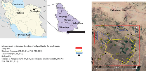
Traditional management systems (smallholder), semi-traditional management systems (total owner), and agricultural companies are the three main exploitation agricultural systems in Iran. They are different in terms of farm sizes, amounts of agricultural inputs, scientific management, ownership systems, and outputs. These systems may affect the soil quality, which needs to be investigated to improve agricultural management. We hypothesized that the management system affects soil quality, productivity, and crop yield. We investigated these three management systems in Neyshabur plain as a representative arid area in Iran to i) evaluate the effect of different management systems on soil quality in surface (Ap horizon) and soil profile, ii) compare the land suitability for alfalfa in different management systems, and iii) compare the relationship between SQI (surface soil and soil profile) and LI with alfalfa yield in the different management systems (Figure 1).

Figure 1. The location of the soil profile and management system in Neyshabur plain, northeastern Iran.

Materials and method

Study area

The study area (~52 km²) is located between coordinates of 58° 44′ 00″ to 58° 49′ 31″ E longitude and 35° 54′ 15″ to 36° 03′ 22″ N latitude (Figure 1). Neyshabur Plain is one of the important agricultural and industrial plains of Khorasan-Razavi province in northeast Iran. This plain is an example of a common agricultural area in the arid environment of Iran. Population growth, intensive agriculture with limited water and soil resources, low quality of irrigation water, incorrect irrigation methods, and non-optimal use of fertilizers caused land degradation in this area. Rangeland and agriculture are the main land uses in this area. There are three agricultural management systems, including traditional management (smallholder), semi-traditional (total owner), and agricultural company (Binaloud company), covering 2127, 340, and 1215 hectares, respectively. The main crops are cotton, canola, and alfalfa under traditional cultivation in the smallholder system, semi-mechanized alfalfa and canola in the total owner system, and mechanized alfalfa, rapeseed, fodder corn, and barley in the Binaloud Company system. Aridisol is the main order of the soils according to Soil Taxonomy (Soil Survey Staff 2014). Soil parent materials are Quaternary sediments from the surrounding mountains and the Kal-Shour River (Ghaemi et al. 1999). Kal-Shour River in the study area is one of the three tributaries of Kal-Shour Khartouran (the largest river of the central desert of Iran), which originates from the Binaloud Mountains in the north of Neyshabur and passes through the south of Neyshabur along the east-west route. Sometimes, the flooding of this river distributes the sediments (mostly silt and clay) and salts along the river bank. The Neogene evaporates in the area have caused the soil salinity of water wells and subsequent agricultural soils.

Soil sampling and analysis

The procedure of this research has been illustrated in Figure 2. Based on field observations and types of management systems, 21 soil profiles were studied in the management systems (Figure 1). The samples were taken in September. Considering the environmental characteristics and management systems, the location and number of samples were selected to cover soil variations. In this study, the surface soil means the Ap horizon in agricultural lands and A in rangelands. The samples from the horizons (0–100 cm) were considered as soil profile. The soil profile is the vertical view of the surface part of the earth’s crust and includes all layers that have undergone pedogenic processes. A horizon is a genetic horizon on the soil surface, where it is a place of accumulation of organic matter. The suffix p in Ap indicates the plow layer. In the study area, due to the differences in the management system and the plow and furrow system, the depth of the Ap horizon was different. In the study area, according to the type of product and root depth, the soil profile depth was considered to be 0 to 100 cm. The significance effect of surface soil properties on plant growth is evident. In addition we assumed that the soil profile characteristics can also have significant effect on soil quality, too. The air-dried samples were ground, sieved (<2 mm), and analyzed for soil properties. Particle size analysis was carried out using the hydrometer method (Gee and Bauder 1986). Soil pH and electrical conductivity were determined in saturated paste and extract, respectively (Thomas 1996). Soil organic carbon (SOC) was determined using the modified Walkley-Black method (Nelson and Sommers 1982), and CaCO₃ equivalent (CCE) was determined using the back-titration method (Allison 1960). Total nitrogen (TN) was determined using the Kjeldahl method (Bremner and Mulvaney 1982). A flame photometer was used to determine soluble sodium (Na_aq), and available potassium (K_av) (Knudsen et al. 1982). A spectrophotometer was used to determine available phosphorus (P_av) (Olsen and Sommers 1982). Alfalfa crop yield data for five years (2014–2019) was obtained from the Department of Agriculture, Government of Neyshabur.

Figure 2. The illustrated procedure of study including date base preparation, data analyses (land suitability and soil quality calculation) and validation the result.

Soil quality evaluation

SQI for the studied management systems was calculated in two depths of surface soil (Ap) and soil profile (0–100 cm) in three stages: a) selection of indicators as MDS by two methods viz., PCA and EO, b) scoring the selected indicators by linear scoring method, and c) calculating SQI by two methods viz., additive and weighted method. The mean value for each characteristic in the soil profile (0–100 cm depth) was calculated using weighted mean and weighting coefficient methods. In the weighting coefficient method, it is assumed that, with increasing soil depth, the importance of soil properties for plant growth decreases. In this method, the soil profile was divided into equal parts with an interval of 25 cm thickness, and a coefficient was assigned to each layer which decreases with depth (Table 1) (Sys et al. 1991). In the weighting coefficient method, it is assumed that, with increasing soil depth, the importance of soil properties for plant growth decreases. It depends both on the depth of the limiting layer, and the crop type. If there is no limiting layer, it is considered a depth of 100 cm and 150 cm for crops and trees, respectively. Otherwise, the depth up to the limiting layer is considered. Thus, a 100 cm depth was considered in our calculations.

Table 1. The number of depth sections and weight coefficients for soils with different depths (Sys et al. 1991).

Soil profile depth (cm)	The number of equal parts with 25 cm intervals	Weight coefficients from top to depth
25	1	1
50	2	1.25–0.75
75	3	1.5-1-0.5
100	4	1.75-1.25-0.75-0.25
125	5	1.5-1.75-1- 0.5-0.25
150	6	2-1.5-1-0.75-0.5-0.25

Indicator selection

Expert opinion (EO) method

In this method, questionnaires were filled by acquiring the information from the farmers and local experts. The analytic hierarchy process (AHP) method was applied to select the minimum data set (Saaty 2008). The purpose of the questionnaire was to understand how each of the soil properties such as EC, Na, SAR, clay, CaCO₃, P, N, K and pH affect soil quality and to what extent they are important.

Principal component analysis (PCA)

In this method, the minimum data set for the surface soil and soil profile was selected using SPSS software, version 22. The objective of PCA was to reduce the dimension of data while minimizing the loss of information (Armenise et al. 2013). Principal components (PC) with high eigenvalues were considered the best representatives of explaining the variability (Andrews et al. 2001).

Scoring the indicators

Selected indicators in MDS of surface soil and soil profile were scored into dimensionless values ranging from 0 to 1 using the linear scoring method (Liebig et al. 2001). Indicators were ranked in ascending or descending order depending on whether a higher value was considered ‘good’ or ‘bad’ in terms of soil function. For ‘higher is better’ indicators such as OC, each value of the indicator was divided by the highest value such that the highest value received a score of 1 (Eq. 1(1) $\mathrm{S}\mathrm{L}=\left(\mathrm{x}-\mathrm{m}\right)/\left(\mathrm{n}-\mathrm{m}\right)$(1) ). For ‘less is better’ indicators such as EC, Na, and SAR the lowest value was divided by each data value such that the lowest value received a score of 1 (Eq. 2(2) $\mathrm{S}\mathrm{L}=1-\left(\left(\mathrm{x}-\mathrm{m}\right)\left(\mathrm{n}-\mathrm{m}\right)\right)$(2) ). For indicators like clay, CaCO₃, P, N, K, and pH, ‘optimum’ threshold value was considered. They were scored as ‘higher is better’ up to a threshold value (e.g. pH 7.5) and then scored as ‘lower is better’ above the threshold (Andrews et al. 2002; Malakouti 2014). Therefore, the more is better, or the less is better equation was applied to score indicators depending on whether the variable value was below or above the threshold value (optimal range). If the indicator’s value was equal to the optimum range, the indicator’s score was calculated by Equation 1.(1) $\mathrm{S}\mathrm{L}=\left(\mathrm{x}-\mathrm{m}\right)/\left(\mathrm{n}-\mathrm{m}\right)$(1)

(1) $\mathrm{S}\mathrm{L}=\left(\mathrm{x}-\mathrm{m}\right)/\left(\mathrm{n}-\mathrm{m}\right)$(1)

(2) $\mathrm{S}\mathrm{L}=1-\left(\left(\mathrm{x}-\mathrm{m}\right)\left(\mathrm{n}-\mathrm{m}\right)\right)$(2)

In the above equations, SL is the linear score between 0 and 1, x is the variable value, m is the minimum value, and n is the maximum value of each indicator (Masto et al. 2008; Askari and Holden 2015).

SQI calculation

Additive index

The additive index was calculated by adding the transformed scores for selected indicators of both PCA and EO (Eq. 3(3) $\mathrm{S}\mathrm{Q}\mathrm{I}\mathrm{A}={\sum }_{\mathrm{i}=1}^{\mathrm{n}}\mathrm{s}\mathrm{i}/\mathrm{n}$(3) ).

(3) $\mathrm{S}\mathrm{Q}\mathrm{I}\mathrm{A}={\sum }_{\mathrm{i}=1}^{\mathrm{n}}\mathrm{s}\mathrm{i}/\mathrm{n}$(3)

Weighted index

The weighted index was calculated by equation 4(4) $\mathrm{S}\mathrm{Q}\mathrm{I}\mathrm{W}={\sum }_{\mathrm{i}=1}^{\mathrm{n}}\mathrm{s}\mathrm{i}\times \mathrm{w}\mathrm{i}$(4) . The transformed indicator data was given weightage based on the results of PCA. Each PC explained a certain amount (%) of the variation in the total dataset. The total percentage of variance from each PC was divided by the percentage of cumulative variance to derive the weightage factor (Ray et al. 2014). The derived weighting coefficient was used with selected variables (indicators) from respective PCs. The weighted variables were then summed up to derive index values for all soil horizons. The weight assignment for the indicators selected by the EO method was the AHP method.

(4) $\mathrm{S}\mathrm{Q}\mathrm{I}\mathrm{W}={\sum }_{\mathrm{i}=1}^{\mathrm{n}}\mathrm{s}\mathrm{i}\times \mathrm{w}\mathrm{i}$(4)

In equations 3(3) $\mathrm{S}\mathrm{Q}\mathrm{I}\mathrm{A}={\sum }_{\mathrm{i}=1}^{\mathrm{n}}\mathrm{s}\mathrm{i}/\mathrm{n}$(3) and 4(4) $\mathrm{S}\mathrm{Q}\mathrm{I}\mathrm{W}={\sum }_{\mathrm{i}=1}^{\mathrm{n}}\mathrm{s}\mathrm{i}\times \mathrm{w}\mathrm{i}$(4) , Si is the non-linear or linear scores of the indicators, n is the number of variables, and WI is the weight of the variables (Masto et al. 2008).

Land suitability assessment for alfalfa

Due to the development of animal husbandry in the region, the alfalfa crop is widely cultivated. On the other hand, it is also present in all three management systems; therefore, alfalfa was selected to evaluate land suitability. The land characteristics, including climate, soil, and topography characteristics, were rated to assess land suitability for irrigated alfalfa (Givi 1998). The degree of suitability of land characteristics was determined by comparing the characteristics’ values to the rated land use requirement of alfalfa. Then, the climate and land indices were calculated to determine land suitability classes.

Climate index and land index

The land index was calculated using the degree of suitability of climate and soil. First, based on equation number 5, the climate index was calculated with the characteristics of rainfall, temperature, and relative humidity of the air. Then, according to equations 6(6) $\mathrm{C}\mathrm{R}=16.67+0.9\mathrm{C}\mathrm{I}$(6) and 7(7) $\mathrm{C}\mathrm{R}=16.6\mathrm{C}\mathrm{I}$(7) , the degree of climate suitability was calculated. Next, based on Table S1 (Givi 1998), soil and topography requirements were estimated. Finally, the land index was calculated by including the suitability degree of climate and soil and topography requirements in equation 5(5) $\mathrm{I}=\mathrm{R}\mathrm{m}\mathrm{i}\mathrm{n}\times \sqrt{\frac{\mathrm{A}}{100}\times \frac{\mathrm{B}}{100}\times \frac{\mathrm{C}}{100}\times \dots }$(5) .

Climate and land indices were calculated by the square root method (equation 5(5) $\mathrm{I}=\mathrm{R}\mathrm{m}\mathrm{i}\mathrm{n}\times \sqrt{\frac{\mathrm{A}}{100}\times \frac{\mathrm{B}}{100}\times \frac{\mathrm{C}}{100}\times \dots }$(5) ) for alfalfa (FAO 1976).

(5) $\mathrm{I}=\mathrm{R}\mathrm{m}\mathrm{i}\mathrm{n}\times \sqrt{\frac{\mathrm{A}}{100}\times \frac{\mathrm{B}}{100}\times \frac{\mathrm{C}}{100}\times \dots }$(5)

Which ‘I’ is the climate index (CI) or land index (LI), Rmin is the lowest degree obtained between climatic and soil characteristics, A, B, C, and … are the degree of other characteristics. For calculating CI, only the climate characteristics were used. The land index was calculated using climate and soil ratings.

A) If the climate index is between 25 and 92.5, climate rating (CR) is calculated with Eq (6)(6) $\mathrm{C}\mathrm{R}=16.67+0.9\mathrm{C}\mathrm{I}$(6) .

(6) $\mathrm{C}\mathrm{R}=16.67+0.9\mathrm{C}\mathrm{I}$(6)

B) If the climate index is < 25, climate rating (CR) is calculated with Eq (7)(7) $\mathrm{C}\mathrm{R}=16.6\mathrm{C}\mathrm{I}$(7) .

(7) $\mathrm{C}\mathrm{R}=16.6\mathrm{C}\mathrm{I}$(7)

C) Based on Table S1 (Sys et al. 1991), soil and topography requirements were estimated for high suitability.

Yield of alfalfa

Predicted alfalfa yield

The predicted yield was calculated using the potential production (Sys et al. 1991) and the Land index (LI). Potential production is the quantity of product assessed based on environmental parameters such as temperature and the amount of energy entering each zone or location. It is not affected by water, soil, management, and pest characteristics. The Potential production of each product is calculated according to climatic data. Since the alfalfa is a perennial crop, this potential was calculated for one year from early April to early October. Plant requirements to use in the method (FAO 1976) were the length of the growth period, leaf area index at the maximum growth rate, harvest index, plant photosynthesis (C3 and C4 plant), and the sensitivity of the plant growth period to the amount of thermal energy and temperature. The potential production was calculated using equations 8(8) $\mathrm{Y}=\mathrm{B}\mathrm{n}\times \mathrm{H}\mathrm{I}$(8) to 10.

(8) $\mathrm{Y}=\mathrm{B}\mathrm{n}\times \mathrm{H}\mathrm{I}$(8)

In equation 8(8) $\mathrm{Y}=\mathrm{B}\mathrm{n}\times \mathrm{H}\mathrm{I}$(8) , Y is the radiation thermal production potential, Bn is the net biomass production, and HI is the harvest index.

(9) $\mathrm{B}\mathrm{n}=\hspace{0.17em}\frac{0.36\times \mathrm{b}\mathrm{g}\mathrm{m}\times \mathrm{K}\mathrm{L}\mathrm{A}\mathrm{I}}{\left(\left(\frac{1}{\mathrm{L}}\right)+0.25\times \mathrm{C}\mathrm{t}\right)}$(9)

(10) $\mathrm{C}\mathrm{T}=\mathrm{C}30\left(0.044+0.0019\mathrm{T}+0.001\times \mathrm{T}2\right)$(10)

In these equations, bgm is the respiration, K is the correction factor, LAI is the leaf area index, L is the growth period, C_T is the intake factor, T is the mean temperature of the growing cycle, and C30 is a factor that is 0.018 for non-legumes and 0.0283 for legumes.

Predicted yield or land potential yield is also observed after water and soil constraints, provided management is also at an excellent level and does not create constraints. For this purpose, radiation thermal production potential was calculated by Eq (8)(8) $\mathrm{Y}=\mathrm{B}\mathrm{n}\times \mathrm{H}\mathrm{I}$(8) and then estimated by the soil index using Eq (11)(11) $\mathrm{P}\mathrm{Y}=\mathrm{Y}\times \mathrm{L}\mathrm{I}$(11) .

(11) $\mathrm{P}\mathrm{Y}=\mathrm{Y}\times \mathrm{L}\mathrm{I}$(11)

In equation 11(11) $\mathrm{P}\mathrm{Y}=\mathrm{Y}\times \mathrm{L}\mathrm{I}$(11) , PY is the predicted yield, Y is the radiation thermal production potential, and LI is the soil index.

Observed alfalfa yield

The crop yield or observed yield is the average production (kg ha⁻¹ a⁻¹). Predicted yield is also called potential land yield. This yield never reaches the potential production because the limitations of water, soil, and the type of management system of the farmer reduce its amount.

Management index

The potential production of land is equal to the yield in which water and land are not limited, and the management is at an excellent level. The crop yield never reaches its potential production because water, soil, and management limitations reduce its yield. Givi (1998) has provided a method to determine the level of land management based on the ratio of observed yield to potential production. The management index is defined as the ratio of observed yield (Y1) to potential production (Y2) (Eq. 12(12) $\mathrm{M}\mathrm{I}=Y1/\mathrm{Y}2$(12) ). MI is the management index, Y2 is the production potential, and Y1 is the observed yield.

(12) $\mathrm{M}\mathrm{I}=Y1/\mathrm{Y}2$(12)

Results

Soil properties

A summary of descriptive statistics for the soil characteristics is provided in Table 2. Most surface soil properties have been affected by climate and parent material and showed more variability than soil profile characteristics (Table 2). EC and clay content had the highest coefficient of variation (CV), with 69 and 44% for the surface soil and soil profile, respectively. The variabilities of TN, K_av, P_av, and SOC were more affected by management. In contrast, EC, Na_aq, and SAR were influenced by irrigation water quality and sediment origin. Rangelands (P₁₀) had the highest SOC, Na_aq, clay, and EC in surface soil and soil profile (Table 3) compared to agricultural lands. The amount of TN, K_av, and P_av in the soils of Binaloud Company and the total owner systems were more than the smallholders and rangelands.

Table 2. Descriptive statistics of the soil properties in the study area.

	Surface				Profile
Soil indicator	Mean	Std.dev	Range	CV (%)	Mean	Std.dev	Range	CV (%)
Naaq (mmol l^−1)	6.5	4.2	13-5.1	53	8.1	5.3	8.2-13.60	37
EC (dS m^−1)	4.2	6.4	9.31 -3	69	4.4	1.1	7.6 -3.3	24
TN (mg kg^−1)	31	5	40- 20	50	23	3	10 -35	8
Pav (mg kg^−1)	9	5.5	15-3	51	6	2.17	2- 10.5	27
Kav (mg kg^−1)	140	5.50	280-70	56	70	533	50-225	34
Silt (%)	22.70	7.3	38-11	58	21.84	5.80	13-38	26
Sand (%)	68	7.9	82-50	67	58.15	11.75	34-78	20
Clay (%)	9.5	6.4	25-2	53	18.96	9.4	7-45	44
SOC (%)	0.30	5.1	0.37-0.30	58	0.18	4.8	0.28 -0.18	31
CCE (%)	17.6	2.50	22– 12	14	15.87	2.3	13-21	14
SAR	2.1	1.70	5.40 -0.2	51	2.82	1.65	1.15-6.20	42
pH	7.80	0.12	8 – 7.50	9	7.7	0.36	8.4-6.7	4

CV: Coefficient of variance, Std.dev: Standard deviation, Na_aq: Soluble sodium, EC: Electrical conductivity, TN: Total nitrogen, P_av: Available phosphorous, K_av: Available potassium, SOC: Soil organic carbon CCE: Calcium carbonate equivalent, and SAR: Sodium absorption ratio.

Table 3. Mean values properties of the representative soil profiles in different management systems.

Surface					Profile
Soil profile	P10	P13	P12	P2	P10	P13	P12	P2
Management system	Rangeland	Smallholder	Total owner	Binaloud company	Rangeland	Smallholder	Total owner	Binaloud company
Naaq (mmol l^−1)	11	5.65	5.4	6.1	7.6	6.40	5.4	6
EC (dS m^−1)	9.3	4.50	4.1	3.6	4.7	5.3	4.13	3.3
TN (mg kg^−1)	13	21	28	36	13	16	20	30
Pav (mg kg^−1)	2	4	12	10	5	6	7	8
Kav (mg kg^−1)	63	66	215	230	60	67	180	178
Silt (%)	10	8	13	18	12	12	10	12
Sand (%)	30	34	40	68	40	38	44	53
Clay (%)	60	58	47	14	50	48	46	35
SOC (%)	0.37	0.30	0.35	0.36	0.28	0.18	0.20	0.20
CCE (%)	21.25	18.5	16.8	15	16.30	15.5	14.30	16.40
SAR	5.45	1.8	1.65	0.9	0.5	0.30	0.20	0.2
pH	8	7.9	7.7	7.7	7.7	7.65	7.75	7.7

Na_aq: Soluble sodium, EC: Electrical conductivity, TN: Total nitrogen, P_av: Available phosphorous, K_av: Available potassium, SOC: Soil organic carbon CCE: Calcium carbonate equivalent, and SAR: Sodium absorption ratio.

Soil quality indicators

MDS selection by EO

Experts and farmers selected the EC, SOC, P_av, K_av, and TN as the most important soil properties. They believed these characteristics distinctly affect the soil quality and crop yield in the area. Due to the small area, the impact of management systems on these characteristics was more than the dry climate and uniform geology. The CCE had a narrow range distribution and had not been selected by the experts.

MDS selected by principal component analysis

Surface soils

For the soil surface, four components with eigenvalues > 1 were selected. These PCs accounted for 33.88, 22.96, 13.22, and 10.18% of the variances and 80.26% of the total variances (Table 4). The selected soil parameters of PC1 were EC and sand. They were significantly correlated (r = −0.56, P-value <0.01) (Table S2), only EC with the highest factor loading was retained in the MDS. The TN and SOC were chosen from PC2, and according to the correlation coefficient between these parameters (0.64, P-value <0.01) (Table S2), SOC with higher loading remained in the MDS. Clay and pH were selected as indicators of PC3 and PC4, respectively, because they had the highest factor loading (Table 4).

Table 4. Results of four principal component analysis of the surface soil properties affecting soil quality.

Principal components	PC1	PC2	PC3	PC4
Eigenvalue	4.067	2.29	1.77	1.23
Variance (%)	33.88	19.100	14.79	10.24
Cumulative variance (%)	33.88	49.65	64.43	74.69
Factor loadings (Rotated component matrix)
Naaq (mmol l^−1)	0.607	-0.689	0.185	0.192
EC (dS m^−1)	0.878	-0.388	-0.104	0.063
Silt (%)	0/779	0.131	-0.571	-0.056
Sand (%)	- 0.870	-0.251	-0.005	0.363
Clay (%)	0.216	0.189	0.782	-0.456
TN (mg kg^−1)	0.050	0.762	0.100	0.354
Kav (mg kg^−1)	0.619	0.125	0.197	-0.399
Pav (mg kg^−1)	-0.452	0.567	0.398	0.116
SOC (%)	0.414	0.769	0.106	0.070
CCE (%)	0.779	0.250	0.137	0.208
SAR	0.209	-0.623	0.603	0.316
pH	0.505	0.235	0.120	0.627

Bold face factor loadings were considered highly weighted and underlined were retained in MDS, Na_aq: Soluble sodium, EC: Electrical conductivity, TN: Total nitrogen, P_av: Available phosphorous, K_av: Available potassium, SOC: Soil organic carbon CCE: Calcium carbonate equivalent and SAR: Sodium absorption ratio.

Soil profile (weighting coefficient)

According to the PCA results of the soil profiles (Table 5), the first five components had eigenvalues > 1. These components explained 30.55, 19.100, 14.79, 10.24, and 9.43% of the variances and 84.12% of the total variances, respectively. Na_aq and silt had the highest loadings in PC1 (Table 5). Considering the significant correlation between these parameters (0.60, P-value <0.01) (Table S3) only, Na_aq with the higher factor loading was retained in the MDS. Clay, SOC, and pH were selected as indicators from PC2, PC3, and PC4, respectively, because they were the only higher-weighed parameters in each PC. K_av and P_av were chosen from PC5, and due to a non-significant correlation between them, both parameters were included in MDS.

Table 5. Results of five principal component analysis of the soil profile properties (weighting factor) affecting soil quality.

Principal components	PC1	PC2	PC3	PC4	PC5
Eigenvalue	3.66	2.29	1.77	1.23	1.13
Variance (%)	30.55	19.100	14.79	10.24	9.43
Cumulative variance (%)	30.55	49.65	64.43	74.69	84.12
Factor loadings (Rotated component matrix)
Naaq (mmol l^−1)	0.830	0.201	-0.296	0.256	-0.180
EC (dS m^−1)	0.555	0.492	-0.392	0.037	0.254
Silt (%)	0.808	-0.121	0.162	-0.226	-0.053
Sand (%)	-0.656	0.680	-0.135	0.081	-0.096
Clay (%)	0.239	-0.842	-0.022	0.044	0.133
TN (mg kg^−1)	0.444	0.344	0.555	0.286	-.0399
Kav (mg kg^−1)	0.626	0.110	0.205	-0.485	-0.464
Pav (mg kg^−1)	-0.344	0.684	0.127	0.132	0.497
SOC (%)	0.124	0.225	0.892	-0.107	-0.208
CCE (%)	0.546	0.148	0.259	0.285	0.427
SAR	0.688	0.220	-0.448	0.293	-0.236
pH	-0.121	-0.381	0.243	0.768	0.318

Bold face factor loadings were considered highly weighted and underlined were retained in MDS, Naaq: Soluble sodium, EC: Electrical conductivity, TN: Total nitrogen, Pav: Available phosphorous, Kav: Available potassium, SOC: Soil organic carbon CCE: Calcium carbonate equivalent and SAR: Sodium absorption ratio.

Soil profile (weighted mean)

In this approach, four components with eigenvalues > 1 were selected. Accordingly, these components explained 38.58, 18.28, 11.80, and 10.23% of the variances, respectively (Table 6). The soil parameters selected from PC1 were Na_aq and SAR. Considering the significant correlation between these parameters (0.72, P value < 0.01) (Table S4), the Na_aq with the higher loading was selected for MDS. The sand and clay in PC2 were significantly correlated (Table S4), and clay with the higher loading was retained in the MDS. pH and TN were selected as indicators from PC3 and PC4, respectively, because they were the higher weighted parameters in each PC.

Table 6. Results of four principal component analysis of the soil profile properties (weighted mean) affecting soil quality.

Principal components	PC1	PC2	PC3	PC4
Eigenvalue	4.63	2.19	1.41	1.22
Variance (%)	38.58	18.28	11.80	10.23
Cumulative variance (%)	38.58	56.87	68.67	78.91
Factor loadings (Rotated component matrix)
Naaq (mmol l^−1)	0.867	0.278	0.270	-0.046
EC (dS m^−1)	0.672	0.333	0.351	-0.055
Silt (%)	0.783	-0.277	0.173	-0.113
Sand (%)	-0.528	0.800	0.038	-0.035
Clay (%)	0.146	-0.821	0.243	0.255
TN (mg kg^−1)	0.558	0.049	-0.384	-0.638
Kav (mg kg^−1)	0.616	-0.292	-0.241	-0.441
Pav (mg kg^−1)	-0.553	0.398	0.037	0.319
SOC (%)	0.681	0.084	-0.339	0.546
CCE (%)	0.659	0.457	-0.291	-0.175
SAR	0.787	0.391	0.215	-0.078
pH	0.019	0.044	0.823	0.326

Bold face factor loadings were considered highly weighted and underlined were retained in MDS, Na_aq: Soluble sodium, EC: Electrical conductivity, TN: Total nitrogen, P_av: Available phosphorous, K_av: Available potassium, SOC: Soil organic carbon CCE: Calcium carbonate equivalent and SAR: Sodium absorption ratio.

SQI in the management system

In the EO method, the weighted index resulted in a higher SQI than the PCA method in all management systems for surface soil and profile (Table 7). The highest additive and weighted EO SQIs were found in the total owner management system. The PCA method found the highest additive and weighted SQIs in the rangelands due to the retaining of SOC compared to agricultural lands.

Table 7. Soil quality index of the different management units in the MDS.

PCA							EO
	Profile						Profile
	Weighted factor		Weighted mean		Surface		Weighted factor		Weighted mean		Surface
Mnagement system	Add	Wi	Add	Wi	Add	Wi	Wi	Add	Wi	Add	Add	Wi
Range lands	0.58	0.59	0.53	0.56	0.45	0.56	1.03	0.46	0.69	0.58	0.58	1.01
Binaloud company	0.57	0.56	0.49	0.53	0.49	0.53	0.89	0.56	0.88	0.52	0.52	0.86
Total owner	0.59	0.59	0.57	0.61	0.52	0.61	1.05	0.58	0.93	0.56	0.56	0.90
Smallholder	0.55	0.54	0.48	0.52	0.47	0.52	0.90	0.56	0.90	0.50	0.50	0.75

Based on Duncan’s mean comparison test (P-value <3%), in both EO and PCA methods, there was a significant difference between the weighted and additive index of surface soil quality between the total owner, rangeland, and the lands of the Binaloud company with the smallholder. However, in each management system, only in the EO method a significant difference was found between the weighted and additive surface SQIs.

The EO SQI had a significant difference between different management systems in terms of the weighted index of surface soil quality (P-value <0.04) and soil profile (P-value <0.03). A significant difference was observed in each management system between the weighted SQI in the EO method (P-value <.05) and other indices. In contrast, in the PCA method, no significant difference was observed between the weighted index of surface soil and soil quality in any management systems.

Land suitability, predicted and observed yield for alfalfa

The calculated class of climate suitability for alfalfa was S1. Integration of the climate with soil and topography characteristics resulted in a moderate land suitability class (S2) for alfalfa cultivation with the soil depth limitation (d) for all soil profiles and salinity limitation (a) for profiles 2, 7, 10, 13 and 8 (Table 8). The limiting depth layer was a compact layer in 30 to 75 cm depth, which was too hard for root penetration.

Table 8. Land suitability for alfalfa in the study area.

Soil profile	Management system	Land index	Predicted yield (kg ha^−1 a^−1)	Observed yield (kg ha^−1 a^−1)	Subclass	Management index
P1	Range lands	73.56	9320	-	S2 d	-
P17		70.04	9160	-	S2 d	-
P4		71.23	9280	-	S2 d	-
P10		69.45	9001	-	S2 da	-
P2	Binaloud company	81.67	9210	8700	S2 da	0.94
P3		80.96	9180	8500	S2 da	0.92
P16		80.65	9150	8400	S2 da	0.91
P18		71.06	9170	8300	S2 d	0.90
P20		69.81	9080	7500	S2 d	0.94
P7	Total owner	60.51	7780	6500	S2 da	0.83
P8		53.06	6890	6250	S2 da	0.90
P12		70.05	9170	7200	S2 d	0.78
P6	Smallholder	60.43	7750	5100	S2 d	0.65
P9		60.45	7150	5200	S2 da	0.72
P11		69.23	9120	6500	S2 da	0.71
P13		55.87	7100	5200	S2 da	0.73
P14		68.21	8900	5700	S2 d	0.64
P15		69.01	9030	6300	S2 d	0.69

The predicted yield for alfalfa was calculated to be 13,500 kg ha⁻¹ a⁻¹ by applying the limitation of land properties (land index) to the heat-radiation potential. The predicted yield was more than the observed yield, and the difference could be attributed to the level of farmers’ management practices. The observed yields in management systems are presented in Table S4. Givi and Haghighi (2016) found that the difference between the crop yield and the predicted yield of rapeseed in Shahrekord (in western Iran) was due to inappropriate planting date, lack of proper application of fertilizer, pesticides, and weed control, and mismanagement of irrigation. Yadollahi Noshabadi et al. (2017) compared the predicted yield of alfalfa (26,800 kg ha⁻¹ a⁻¹), the observed yield (16,000 kg ha⁻¹ a⁻¹), and the yield of eminent farmers (25,000 kg ha⁻¹ a⁻¹) in Alborz Province in Iran. They suggested the promotion of the management, optimal use of water resources, and the removal of modifiable soil constraints to achieve the predicted yield.

The regression relationship between the predicted yield and observed yield of alfalfa was calculated in management systems (Figure 3). The high regression relationship, especially in the total owner management system (R² = 0.88) and Binaloud Company (R² = 0.80), shows the high accuracy of the evaluation method and the high level of farmers’ management practices. Usually, farmers’ yield is different in the same climatic, soil, and topography conditions. On the other hand, in most cases, there is no agreement between the predicted and observed yield, due to management differences (Ayoubi and Jalalian 2016). They examined the regression relationship between the predicted and observed yield, in which the high R² value (0.68) indicated the acceptable accuracy of the methods used for land suitability assessment. El Baroudy (2016) expressed a strong relationship between observed and predicted yield (R² = 0.89).

Figure 3. Relationship between the observed yield and predicted yield in the management systems.

Relationship between yield and indices

Observed yield and SQI

Identifying relationships between soil properties and crop yields is necessary to improve management and cultivation practices, as well as to validate the land suitability evaluation procedure (Bagheri Bodaghabadi et al. 2019). In the EO method, for the total owner management system, the weighted SQI of both surface soil and soil profile had a good relationship with observed yield (Table 9) and justified more than 50% of the yield variations. The rest could be due to differences in management system attributes such as planting date, fertilizer inputs, and quantity/quality of irrigation water. The reason for the better relationship between EO-SQI and alfalfa yield can be attributed to the fact that PCA is a data reduction procedure, whereas, in contrast, the MDS in the EO method was selected by experts who were aware of the cause-and-effect relationship between soil and plant. Vasu et al. (2016) reported a significant correlation between SQI and chickpea yield in the PCA method and cotton and corn yields in the EO method. Ranjbar et al. (2016) compared the integrated quality index (IQI) and Nemoro quality index (NQI) methods in estimating SQI and showed that the correlation between saffron yield and SQI was not significant. Mukherjee and Lal (2014) used three methods for determining the SQI in Ohio. They indicated that due to the appropriate weight for soil properties, the weighted SQI was better correlated with observed yield compared to the additive SQI. Liu et al. (2014) determined the soil quality of Chinese paddy lands and showed a significant correlation between the SQI and rice yield.

Table 9. Regression relationship between surface and profile soil quality index with observed yield of alfalfa in the MDS.

		EO				PCA
Depth	Management system	Weighted		Additive		Weighted		Additive
Surface	Binaloud company	0.49		0.46		0.17		0.12
	Total owner	0.52		0.50		0.20		0.13
	Smallholder	0.35		0.32		0.14		0.09
		Weighted factor		Weighted mean		Weighted factor		Weighted mean
Profile		Weighted	Additive	Weighted	Additive	Weighted	Additive	Weighted	Additive
	Binaloud company	0.44	0.40	0.43	0.40	0.44	0.42	0.31	0.27
	Total owner	0.66	0.65	0.66	0.63	0.56	0.53	0.62	0.60
	Smallholder	0.63	0.56	0.60	0.50	0.36	0.38	0.34	0.33

Observed yield and land index

We observed a significant positive relationship between alfalfa yield and land index in all three of the studied management systems (Figure 4). The higher yield in Binaloud Company compared to other management systems was due to proper management and high production inputs. However, it should be noted that this land utilization type may not be sustainable. Seyedmohammadi et al. (2019) evaluated and showed that the relationship between the land index and barley observed yield in combination with the AHP and GIS method (R² = 0.94) was more accurate than the Storie and parametric (square root) methods. Vasu et al. (2018) showed that the correlation between the land index and observed yield with R² values of 0.78 for chickpea, 0.63 for corn, and 0.56 for rice and multi-criteria methods were better than the Storie and parametric methods. Since the climate in the present study is not a limiting factor, the R² values between the observed yield and land index could be a function of soil characteristics. For the land suitability assessment, rated climate and soil characteristics for alfalfa growth were used to calculate the land index. In contrast, those characteristics were used for soil quality assessment, which varied due to differences in management systems. Therefore, regression analysis indicated a better relationship between land indexes and observed yield than SQI (Figure 4) (Table 9).

Figure 4. Relationship between the observed yield and land index in the management systems.

Management index

Determining an indicator for quantifying the management is very difficult due to the complexity of management. However, it is possible to determine the management index regionally (Givi 1998). Binaloud Company and the total owner lands, with a management index > 0.75, were good despite the limitation of soil and water salinity and a limiting layer. Smallholder lands with a management index of < 0.75 showed a moderate management level. The decline in yield was initially due to salinity and soil depth limitations. However, applying suitable management practices, especially salinity management in the lands of Binaloud Company and the total owner, was efficiently achieved more yield.

Discussion

Variation of soil characteristics

Considering the dry climate and nearly homogenous soil parent material, natural factors (mostly climate and parent materials) and management practices have affected the soil characteristics and profile. The sediments and hydrology of the seasonal Kal-Shour River affect the variability and distribution of most soil characteristics in the area. The suitable depth for plant growth and the amount of sand increases with distance from the Kal-Shour River, and the amount of clay, soluble sodium, and EC decreases. In this regard, Mirakzehi et al. (2018) showed that river activities were one of the main factors influencing soil formation and development in the Hirmand River delta in eastern Iran. Pahlavan-Rad et al. (2018, 2020) showed that channel networks and distance from the river significantly affect soil properties. Through digital soil mapping, they used these features as the most important auxiliary variables to estimate soil permeability and soil organic carbon. In rangeland, the salinity of the surface soil was higher than the underlying layers due to lack of irrigation, low rainfall, and high evapotranspiration in the region.

In contrast, the salinity of underlying layers was higher due to the EC of irrigation water (Table S5) and proximity to Kal-Shour River. For example, profile 10 in rangeland had the highest EC on the surface (9.3 dS m⁻¹) due to its proximity to the Kal-Shour River (Table 2). Profile 13 in agricultural lands with smallholder management had a higher EC in the subsurface (average profile, 5.3 dS m⁻¹) than the surface (4.50 dS m⁻¹) due to irrigation and cultivation despite being close to the Kal-Shour River. In profile 12, with agricultural use but total owner management and close to Kal-Shour River, the EC was relatively high but less than the smallholder land (average profile, 4.23 and surface, 1.4 dS m⁻¹). Ayoubi et al. (2009) showed that the variability of soil characteristics could be influenced by both internal factors (soil factors, including parent materials) and external factors (type of management).

Soil quality index and soil organic carbon

Among the soil characteristics, organic carbon is the factor that affects most of the soil properties and soil quality. In this regard, Vasu et al. (2016) showed that organic carbon is one of the most important soil characteristics regardless of the soil and crop management strategy due to its important role in the properties of the soil. Since more than 80% of Iran’s area is in arid and semi-arid climates (Bagheri Bodaghabadi et al. 2019), the soil organic carbon content is less than 1%. Considering the region’s dry climate, the amount of organic carbon in the soil was low and controlled by the type of management systems. The soil organic carbon in surface soil and soil profile was 0.37 and 0.28% in rangeland, 0.30 and 0.18% in smallholder lands, 0.35 and 0.20 in total owner lands, and 0.36 and 0.20% in the lands of Binaloud Company. However, it is within the normal range of the soils of dry areas. The increase in organic carbon and the SQI in rangeland is due to the lack of cultivation and conservation of organic carbon compared to agricultural land.

Comparison of the PCA and EO methods for soil quality calculation

In the current study, two methods of EO and PCA were used to select the minimum data set. The results showed that the SQI calculated in the EO method was higher than in the PCA method. This agrees with the findings of Pal et al. (2012, 2013) and Vasu et al. (2016). Although PCA is a widely accepted statistical method for indicator selection, it is still necessary to consider the region’s characteristics and the pedogenic processes that affect productivity (Vasu et al. 2016) so that experts can make a sound judgment to introduce the most important indicators. The relationship between alfalfa yield and the EO weighted SQI in the total owner system (surface soil R² = 0.52 and soil profile R² = 0.66) was more than the smallholder system (surface soil R² = 0.35 and soil profile R² = 0.63). The reason the EO SQI has established a better relationship with crop yield may be that the PCA method is a data dimension reduction method. In contrast, experts who are aware of soil cause and effect, choose the MDS in the EO method. Vasu et al. (2016) expressed the highest correlation between the SQI with peas in the PCA set in the soil profile and with cotton and corn in the EO set.

Soil quality index in surface soil and soil profile

In this study, along with surface soil characteristics, profile characteristics were also used to estimate the SQI. The relationship between the SQI and alfalfa yield was better in the soil profile than in the surface soil (Table 9). Accordingly, considering the soil profile characteristics gives a more comprehensive view of the soil quality, which is consistent with the findings of Hewitt (2004). In the studied area, in both methods of PCA and EO, the SQI in the profile was higher than in the surface soil (Table 7). Vasu et al. (2016) applied surface soil and soil profile characteristics and concluded that integrating surface soil and soil profile information is more suitable for soil quality assessment. Gozukara et al. (2022) showed that the soil characteristics varied significantly with depth and concluded that subsurface properties influence the soil quality.

As stated, soil characteristics and management system variations increase or decrease the soil quality. The soil quality improved with increasing distance from the Kal-Shour River and the management moving from smallholder to total owner, due to the proper land management and the knowledge and awareness of farmers. In the present study, soil quality and crop yield were higher in Binaloud company and the total owner lands than that of the smallholder lands due to the better and more principled management practices such as the supply of organic matter and soil nutrients, better supply of irrigation water, the use of more modern agricultural machinery, increasing the knowledge of experts and managers. In these lands, some farmers obtained low yield due to poor management, while their lands did not have any soil and climate restrictions, and with proper management and weed control, they could have a high yield. Therefore, since smallholder farmers have a significant contribution to production and food security (Oruru and Njeru 2016), it is essential to assess soil quality at the farm scale and assess the contribution of agricultural inputs in formulating policies and technologies to improve smallholder land management practices (Li et al. 2022). Assis and Mohd Ismail (2011) and Kuria et al. (2019) stated the importance of farmers’ knowledge and awareness to sustain soil health and accept the new technology.

In the present study, the weighting coefficient method was also used in addition to the weighted mean method to achieve a single value for each characteristic in the profile. The results showed that the method of weighting coefficient, in comparison to the weighted mean, by applying different weights to each layer, showed a higher SQI in both EO and PCA methods. However, considering that no such comparison has been made so far, it is better to conduct more studies in this field to draw more accurate conclusions.

Soil quality index and land index

In most land suitability evaluation studies, the correlation between the crop yield and the land index is applied to check the validity of the evaluation method (Mousavi et al. 2015; Diyalami et al. 2017. In our study, in addition to the land index, the relationship between crop yield and SQI was also examined (Table 9). Since the land index is calculated based on the crop requirements, compared to the SQI, which considers the general state of soil quality, shows a stronger relationship with the observed yield (Figure 4) (Total owner, R² = 0.96, smallholder R² = 0.72, and Binload company R² = 66). This relationship also showed that the land index could accurately determine the suitability of the land for crop cultivation and identify the characteristics that cause a decrease yield, especially the smallholder system. However, since it is the first attempt to compare these indices, more research is needed to achieve more accurate conclusions.

Conclusions

This study showed that considering the soil profile properties rather than surface soil alone and applying the knowledge of farmers and local experts were more effective in soil quality evaluation. The weighting coefficient method indicated a higher SQI in both EO and PCA. The higher relationship between observed yield and land index than SQI showed that land index could accurately determine the land suitability for a specific crop. In addition, in terms of production, total owner and Binaloud Company management systems showed higher soil quality than the smallholders due to using principled and expert management practices. However, despite the efficiency of the total owner and Binaloud Company, they may be unsustainable due to high inputs of fertilizers and water, which may not be sustainable in the long term. Therefore, further studies are proposed to consider water efficiency in the different management systems.

Acknowledgments

We are grateful to Ferdowsi University of Mashhad Research for financial support of this study (grant no. 3/52516: 1399/04/11).

Disclosure statement

No potential conflict of interest was reported by the author(s).

Supplementary material

Supplemental data for this article can be accessed online at https://doi.org/10.1080/03650340.2023.2298851.

Additional information

Funding

This research was financially supported by the Ferdowsi University of Mashhad Research Council [Grant: 3/52516:1399/04/11].

References

- Abera W., Assen M., Satyal P. 2020. Synergy between farmers’ knowledge of soil quality change and scientifically measured soil quality indicators in Wanka watershed, northwestern highlands of Ethiopia. Environ Develop Sust. 23(2):1316–1334. doi: 10.1007/s10668-020-00622-3.
- Allison L. 1960. Wet combustion apparatus and procedure for organic and inorganic carbon in soil. Soil Sci Soc Am Proc. 24(1):36–40. doi: 10.2136/sssaj1960.03615995002400010018x.
- Andrews SS, Carroll CR. 2001. Designing a soil quality assessment tool for sustainable agro ecosystem management. Ecol Appll. 11:1573–1585.
- Andrews S.S., Karlen D.L., Mitchell J.P. 2002. A comparison of soil quality indexing methods for vegetable production systems in Northern California. Agric Ecosyst Environ. 90(1):25–45. doi: 10.1016/S0167-8809(01)00174-8.
- Aparicio V., Costa J.L. 2007. Soil quality indicators under continuous cropping systems in the Argentinean pampas. Soil Till Res. 96(1–2):155–165. doi: 10.1016/j.still.2007.05.006.
- Armenise E., Redmile-Gordon M.A., Stellacci A.M., Ciccarese A., Rubino P. 2013. Developing a SQI to compare soil fitness for agricultural use under different managements in the Mediterranean environment. Soil Till Res. 130:91–98. doi: 10.1016/j.still.2013.02.013.
- Askari M.S., Holden N.M. 2015. Quantitative soil quality indexing of temperate arable management systems. Soil Till Res. 150:57–67. doi: 10.1016/j.still.2015.01.010.
- Assis K., Mohd Ismail H.A. 2011. Knowledge, attitude and practices of farmers towards organic farming. Int J Ecol Res. 2:1–6.
- Ayoubi S., Jalalian A. 2016. Land evaluation (agriculture and natural resources). second ed. Isfahan: Isfahan University of Technology, Iran. In Persian.
- Ayoubi S., Mohammad Zamani S., Khormali F. 2009. Predicting wheat yield using soil properties using principal component analysis. Iranian J Soil Water Res. 49(1):51–57. In Persian.
- Bagheri Bodaghabadi M., Amini Faskhodi A., Salehi M.H., Hosseinifard S.J., Heydari M. 2019. Soil suitability analysis and evaluation of pistachio orchard farming, using canonical multivariate analysis. Sci Hortic. 246:528–534. doi: 10.1016/j.scienta.2018.10.069.
- Bremner J., Mulvaney C. 1982. Nitrogen total. In: Page A., Miller R. Keeney D., editors. Methods of soil analysis. Part 2: chemical and microbiological properties. Madison, Wisconsin: American Society of Agronomy-Soil Science Society of America, USA; p. 595–624.
- Bünemann EK, Bongiorno G, Bai Z, Creamer RE, De Deyn G, de Goede R, Fleskens L, Geissen V, Kuyper TW, Mäder P, et al. 2018. Soil quality A critical review. Soil Biol Biochem. 120:105–125. doi: 10.1016/j.soilbio.2018.01.030.
- Diyalami H., Givi J., Naderi Khorastegani M. 2017. Comparison of parametric methods and fuzzy hierarchical analysis in order to evaluate land suitability, Dashtestan region of Bushehr province for planting date palms. Agric Eng (Sci J Agric). 41:45–58. In Persian.
- El Baroudy A.A. 2016. Mapping and evaluating land suitability using a GIS-based model. Catena. 140:96–104. doi: 10.1016/j.catena.2015.12.010.
- FAO. 1976. A framework for land evaluation. Soil Bulletin No. 32. Rome.
- Gee G.W., Bauder J.W. 1986. Particle size analysis. In: Klute A., editor. Methods of soil analysis part 1: physical and mineralogical mthods. Second, SSSA Book Series No. 5. Madison, Wisconsin: American Society of Agronomy-Soil Science Society of America, USA; p. 383–412.
- Ghaemi F., Ghaemi F., Hosseini K. 1999. Geological map (1: 100000) of Neyshabur. Geological Survey Of Iran Press. In Persian.
- Givi J. 1998. Qualitative assessment of land suitability for crops and orchards. Tehran: Water And Soil Research Institute, Journal No 1015 Iran. In Persian.
- Givi J., Haghighi A. 2016. Production potential prediction and quantitative land suitability evaluation for irrigated cultivation of canola (Brassica napus) north of shahrekord district. J Water Soil. 29:1651–1661. In Persian.
- Gozukara G., Acar M., Ozlu E., Dengiz O., Hartemink A.E., Zhang Y. 2022. A SQI using vis-NIR and pXRF spectra of a soil profile. Catena. 211:105954. doi: 10.1016/j.catena.2021.105954.
- Hewitt AE. 2004. Soil properties relevant to plant growth: AGuide to recognizing soil properties relevant to plant growth and protection. Lincoln, New Zealand: Manaaki Wenua Press.
- Issanchou A., Karine D., Dupraz P., Ropars-Collet C. 2018. Inter temporal soil management: revisiting the shape of the crop production function. J Environ Plann Man. 62(11):1845–1863. doi: 10.1080/09640568.2018.1515730.
- Karlen D.L., Mausbach M.J., Doran J.W., Cline R.G., Harris R.F., Schuman G.E. 1997. Soil quality: a concept, definition, and framework for evaluation. Soil Sci Soc Am J. 61(1):4–10. doi: 10.2136/sssaj1997.03615995006100010001x.
- Knudsen D., Peterson G.A., Pratt P.F. 1982. Lithium, sodium and potassium. In: Page A., Miller R.H., and Keeney D.R. editors. Methods of soil analysis. Part 2. In: chemical and microbiological properties no. 9. 2nd. Madison, Wisconsin: American Society of Agronomy and Soil Science Society of America, USA; p. 225–245.
- Kuria A., Barrios E., Pagella T., Muthuri C.W., Mukuralindam A., Snclair F.L. 2019. Farmers’ knowledge of soil quality indicators along a land degradation gradient in Rwanda. Geoderma Reg. 16:e00199. doi: 10.1016/j.geodrs.2018.e00199.
- Liebig M.A., Varvel G., Doran J.W. 2001. A simple performance-based index for assessing multiple agroecosystem functions. Agron J. 93(2):313–318. doi: 10.2134/agronj2001.932313x.
- Liu Z., Zhou W., Shen J., He P., Lei Q., Liang G. 2014. A simple assessment on spatial variability of rice yield and selected soil chemical properties of paddy fields in South China. Geoderma. 235-236:39–47. doi: 10.1016/j.geoderma.2014.06.027.
- Li K., Wang C., Zhang H., Zhang J., Jiang R., Feng G., Liu X., Zuo Y., Yuan H., Zhang C., et al. 2022. Evaluating the effects of agricultural inputs on the soil quality of smallholdings using improved indices. Catena. 209:105838. doi: 10.1016/j.catena.2021.105838.
- Malakouti M.J. 2014. Optimal fertilizer recommendation for agricultural products in Iran. TehranIran: Mobaleghan Press. In Persian.
- Maleki S., Karimi A., Zeraatpisheh M., Pouzeshi R., Feizi H. 2021. Long-term cultivation effects on soil properties variations in different landforms in an arid region of eastern Iran. Catena. 206:105465. doi: 10.1016/j.catena.2021.105465.
- Masto R., Chhonkar P., Singh D., Patra A. 2008. Alternative soil quality indices for evaluating the effect of intensive cropping, fertilisation and manuring for 31 years in the semi-arid soils of India. Environ Monit Assess. 136(1–3):419–435. doi: 10.1007/s10661-007-9697-z.
- Mirakzehi K., Pahlavan-Rad M.R., Shariari A., Bameri A. 2018. Digital soil mapping of deltaic soils: a case of study from hirmand (Helmand) river delta. Geoderma. 313:233–240. doi: 10.1016/j.geoderma.2017.10.048.
- Mousavi S.A., Sarmadian F., Taati A. 2015. Comparison of the FAO method and the analytical hierarchy process (AHP) to evaluate land suitability for dry wheat in Kohin region. J Soil Res (Soil Water Sci). 30:367–377. In Persian.
- Mukherjee A., Lal R. 2014. Comparison of SQI using three methods. PLoS ONE. 9(8):1–15. doi: 10.1371/journal.pone.0105981.
- Nelson D.W., Sommers L.E. 1982. Total carbon organic carbon and organic matter. In: Page A., Miller H. Keeney D., editors Methods of soil analysis, part 2. Chemical and microbiological properties. Madison: American Society of Agronomy and Soil Science Society of America, USA; p. 539–577.
- Olsen S.R., Sommers L.E. 1982. Phosphorus. In: Page A., Miller H. Keeney D., editors. Methods of soil analysis, part 2. Chemical and microbiological properties. Madison: American Society of Agronomy and Soil Science Society of America, USA; p. 403–429.
- Oruru M.B., Njeru E.M. 2016. Upscaling arbuscular mycorrhizal symbiosis and related agroecosystems services in smallholder farming systems. Bio Res Int. 2016:1–12. doi: 10.1155/2016/4376240.
- Pahlavan-Rad M.R., Dahmarde K., Hadizadeh M., Keykha G., Mohammadnia N., Gangali M., Keikah M., Davatgar N., Brungard C. 2020. Prediction of soil water infiltration using multiple linear regression and random forest in a dry flood plain, eastern Iran. Catena. 194:104715. doi: 10.1016/j.catena.2020.104715.
- Pahlavan-Rad M.R., Dahmardeh K., Burongard C. 2018. Predicting soil organic carbon concentrations in a low relief landscape, eastern Iran. Geoderma Reg. 15:e00195. doi: 10.1016/j.geodrs.2018.e00195.
- Pal D.K., Sarkar D., Bhattacharyya T., Datta S.C., Chandran P., Ray S.K. 2013. Impact of climate change in soils of semi-arid tropics (SAT). In: Bhattacharyya T., Pal D. Wani S., editors. Climate change and agriculture. New Delhi: Studium Press, India; p. 113–121.
- Pal D.K., Wani S.P., Sahrawat K.L. 2012. Vertisols of tropical Indian environments. Pedology and edaphology. Geoderma. 189-190:28–49. doi: 10.1016/j.geoderma.2012.04.021.
- Ranjbar A., Emami H., Khorasani R., Karimi Karoye A.R. 2016. Soil quality assessments in some Iranian Saffron Fields. J Agr Sci Tech. 18:865–878.
- Ray S.K., Bhattacharyya T., Reddy K.R., Pal D.K., Chandran P., Tiwary P. 2014. Soil and land quality indicators of the Indo-Gangetic Plains of India. Curr Sci. 107:1470–1486.
- Saaty T.L. 2008. Decision making with the analytic hierarchy process. Int J Serv Sci. 1(1):83–98. doi: 10.1504/IJSSci.2008.01759.
- Samaei F., Emami H., Lakzian A. 2022. Assessing soil quality of pasture and agriculture land uses in Shandiz county, northwestern Iran. Ecol Indic. 139:108974. doi: 10.1016/j.ecolind.2022.108974.
- Seyedmohammadi J., Sarmadian F., Jafarzadeh A.A., McDowell R.W. 2019. Development of a model using matter element, AHP and GIS techniques to assess the suitability of land for agriculture. Geoderma. 352:80–95. doi: 10.1016/j.geoderma.2019.05.046.
- Soil Survey Staff. 2014. Keys to Soil Taxonomy. 12th ed. Washington DC: USDA-Natural Resources Conservation Service.
- Sys C., Van Ranst E., Debaveye J. 1991. Land evaluation. Part 1: principles in land evaluation and crop production calculation. General Administration for Development Cooperation, Agric. Publ. No. 7, Brussels.
- Thomas G.W. 1996. Soil pH and soil acidity. In: Sparks D., editor Methods of soil analysis. Part 3: chemical methods, SSSA book series 5. Wisconsin: Soil Science Society of America, Madison, USA; p. 475–490.
- Vasu D., Srivastava R., Patil N.G., Tiwary P., Chandran P., Sing S.K. 2018. A comparative assessment of land suitability evaluation methods for agricultural land use planning at village level. Land Use Pol. 79:146–163. doi: 10.1016/j.landusepol.2018.08.007.
- Vasu D., Tiwary P., Chandran P., Singh S.K. 2016. Soil Quality for Sustainable agriculture. Geoderma. 282:70–79. doi: 10.1016/j.geoderma.2016.07.010.
- Williams H., Colombi T., Keller T. 2020. The influence of soil management on soil health: an on-farm study in southern Sweden. Geoderma. 360:114010. doi: 10.1016/j.geoderma.2019.114010.
- Yadollahi Noshabadi S.J., Jahansoz M.R., Majnon Hosseini N., Peykani G.H.R. 2017. Assessing the production capacity of major crops in the lands of Hashtgerd region using FAO method. Iranian J Field Crop Sci. 48:25–38. In Persian.