The first national scale spatial and temporal analysis of surface CO₂ over South Africa utilising satellite retrievals

ABSTRACT

South Africa is the dominant continental source region of CO₂ fossil fuel emissions. This is a result of the strong dependence of its economy on fossil fuels. However, the observations of atmospheric CO₂ in South Africa are inadequate. The country has the Global Atmospheric Watch (GAW) Cape Point station as the only site with long-term ambient CO₂ monitoring record. In this study, satellite data retrieved from the Tropospheric Emission Spectrometer (TES) instrument on board the Aura satellite from Dec 2004 to Dec 2009 is used for the first time to quantify the spatial distribution of CO₂ over South Africa, as well as to determine its annual variability at selected sites. The study found that the surface CO₂ foot print in South Africa resembles the industrial CO₂ emission sources spatial distribution, particularly during the summer and autumn. In winter and spring seasons the surface CO₂ foot prints are spatially expanded as a result of contributions of emissions from biomass and domestic fossil fuel combustion. The surface levels of CO₂ at the study areas have been increasing during the period of the analysis.

KEYWORDS:

• CO₂
• observations
• emission sources
• spatial distribution
• temporal variation

1. Introduction

Atmospheric CO₂ is a long-lived greenhouse gas (LLGHG), with an atmospheric lifetime of 50 to 200 years (Intergovernmental Panel on Climate Change, 1996). It contributes about 66% of the gaseous radiative forcing responsible for anthropogenic climate change (World Meteorological Organisation, 2018). Among the LLGHGs, CO₂ increases have caused the largest sustained radiative increased forcing over the past decade. It contributed about 84% of the increase in radiative forcing over the past decade and about 83% over the past five years. The globally averaged surface CO₂ reached a new high in 2017 of 405.5 ppm (WMO, 2018) and the Mauna Loa station with the longest global records of CO₂ recorded a historical peak of monthly average of 415 ppm in May 2019 (National Oceanic and Atmospheric Administration, 2020). The increases in global atmospheric CO₂ are mainly due to anthropogenic activities, including combustion of fossil fuel, gas flaring, cement production, and land use changes such as deforestation and biomass burning (Fang et al., 20,014; Forster et al., 2007; IPCC, 1996; Sabine et al., 2004; WMO, 2012, 2013, 2014). This annual accumulation of CO₂ in the atmosphere is a result of partial removal of anthropogenically emitted CO₂ by terrestrial and ocean sinks (Canadell et al., 2007; Le Quéré et al., 2009; Sabine et al., 2004).

The first in situ long-term continuous observations of atmospheric CO₂ began in 1959 at Mauna Loa in Hawaii (Brailsford et al., 2012). The Mauna Loa measurements were followed by a continuous in situ observation programmes at other sites. These observations revealed that the atmospheric CO₂ was increasing annually, and the trend has a seasonal cycle (Fang et al., 2014; Forster et al., 2007). In 2012, there were 121 CO₂ monitoring stations around the world that contributed data towards the computation of CO₂ global atmospheric average (WMO, 2013). However, relatively dense networks are found over North America and Western Europe (Deutscher et al., 2014; Fang et al., 2014). The Southern Hemisphere is under-represented in various passive sampling and continuous monitoring programmes of greenhouse gases (Morgan et al., 2015).

Observations of CO₂ in the African continent are much sparser compared to other continents. There are only two GAW stations in Africa involved in long-term monitoring of ambient CO₂, one located at Cape Point, South Africa (34.35° S, 18.49° E) and the other at Namibia Desert Atmospheric Observatory (NDAO) in Namibia (22.55° S, 15.03° E) near the Gobabeb Training and Research Centre (Brunke et al., 2011; Labuschagne et al., 2018; Morgan et al., 2015; Nickless et al., 2015). Both these stations are predominately impacted by background air; the Cape Point station is dominated by air originating from Southern Ocean and NDAO observes air representative of terrestrial and Atlantic Ocean background (Brunke et al., 2011; Labuschagne et al., 2018; Morgan et al., 2015; Nickless et al., 2015).

Southern Africa led by South Africa is the dominant continental source region of fossil fuel emissions. The region has the highest per capita emission rate of 8.5 Mg CO₂-eq person⁻¹ yr⁻¹, this is 4 to 20 times the per capita emissions of other African regions (Valentini et al., 2014). The continental-wide industrial CO₂ emissions are also small, but they are significant for an industrial country such as South Africa (Williams et al., 2007). South Africa has the biggest industrialized economy in southern Africa (Department of Environmental Affairs, 2014; Freiman & Piketh, 2003). The country has diverse CO₂ emitting sources; the broad range of industries, domestic emissions from fossil fuel use, natural and anthropogenic biomass burning (DEA, 2014). The industrial sources of CO₂ are spread at different sites all over the country, with the majority located at the Highveld region followed by the Limpopo and KwaZulu-Natal province. In South Africa 93% of the electricity needs are provided by fossil fuels, and coal power plants contribute 77% of the country’s electricity needs. Coal power plant operations are responsible for South Africa’s power sector being the 9^th highest CO₂ emitter in the world (Osman et al., 2014).

Given that South Africa takes continental dominance in CO₂ fossil fuel emissions (Valentini et al., 2014), the GAW station at Cape Point, which is located at the southern end of the Cape Peninsula, is the only station with long-term CO₂ monitoring record. There is a general country-wide lack of information regarding CO₂ atmospheric loading. However, efforts are made to close this gap, two new ambient CO₂ stations are commissioned in the northeast of the country (Feig et al., 2017). The two new stations are also aimed at reducing the high uncertainty associated with CO₂ emission flux estimation over the country, from CO₂ measurements from the Cape Point GAW station and inverse modelling (Feig et al., 2017; Nickless et al., 2015).

Because of the lack of long-term CO₂ observation data on a country-wide scale, this study aims to provide the first valuable insight into the seasonal surface spatial distribution of CO₂ over South Africa and the annual variation of surface concentrations of CO₂ at selected areas using TES on-board the Aura Satellite. This study also aims to verify known and identify unknown CO₂ hotspots over the country and assess if their geographic location is in agreement with the latest spatial industrial CO₂ inventory compiled by Osman et al. (2014).

2. Materials and methods

2.1 TES instrument

Quality controlled CO₂ profiles data collected from the TES instrument on-board the Aura satellite were used for analysis. TES is an infrared, high resolution Fourier transform spectrometer (FTS) and it operates in both nadir (downward view) and limb (side view) modes to measure the vertical distribution of atmospheric chemical composition and surface parameters (Beer, 2006; Beer et al., 2001; Jones et al., 2009, 2003; Rinsland et al., 2006; Schoeberl et al., 2006; Worden et al., 2004). A comparison study of TES and aircraft CO₂ profiles established that TES CO₂ measurements error range was 0.8–1.8 ppm depending on atmospheric pressure level and geo-location. The surface correlation of the measurements from the two platforms was greater than 0.85, except at the subtropics (Kulawik et al., 2013). The CO₂ profile data used in this study were provided by the National Aeronautics and Space Administration (NASA) and made available from TES website https://tes.jpl.nasa.gov/data.

2.2 Study sites locations and description

TES nadir view data were analysed within the South African domain, bounded by 17° to 33° E longitude and 22° to 35° S latitude. Seven areas within South Africa were selected to analyse the temporal variation of CO₂. Table 1 and Figure 1 show these areas and their demarcations. The selected study regions were chosen based on major regions of anthropogenic activities in South Africa and their corresponding landscapes.

Figure 1. Map of South Africa showing the position of areas that were analysed for surface CO₂ annual variation.

Table 1. Demarcations of regions analysed for surface annual variation of CO_2.

Area	Latitude range (°S)	Longitude range (°E)
Cape Town (CT) Central Freestate (FS) Central Northern Cape (NC) Coastal Eastern Cape (EC) Coastal KwaZulu-Natal (KZN) Industrial Highveld (IHV) Limpopo (L)	32.5° to 35.0° 27.5° to 29.5° 28.0° to 31.0° 32.0° to 34.5° 28.0° to 31.0° 24.8° to 27.2° 22.0° to 25.0°	17.5° to 20.5° 25.5° to 29.0° 21.0° to 25.0° 25.0° to 29.0° 30.0° to 32.7° 26.8° to 30.2° 27.0° to 32.0°

Cape Town (CT) study area extends from the southwest coast into the interior of Western Cape Province including the City of Cape Town and other towns within the province (Figure 1). The main sources of this region include industry, road traffic, power generation, domestic fuel use and biomass burning (United Nations Development Programme, 2016; Western Cape: Department of Environmental Affairs and Development, 2017).

The central Freestate (FS) area lies at the centre of the country and is overlapping the northwestern part of Lesotho (Figure 1). The economy of this area is dominated by agriculture and mining. The landscape is mainly cultivated land and natural savanna grassland. (Puukka et al., 2012).

The central Northern Cape (NC) (Karoo) area (Figure 1) was selected because it is a national terrestrial background area with regard to CO₂ atmospheric loading. The spatial industrial CO₂ source inventory from Osman et al. (2014) reveals only one industrial CO₂ emissions source and there is no biomass fire emissions in this region (Bond et al., 2003; Silva et al., 2003).

The coastal Eastern Cape (EC) study area lies on the southeast coast of the country. It includes the two metropolitan towns, East London and Port Elizabeth, surrounding small towns and the dense bush land (Figure 1). The area has a rich diverse natural biome. East London and Port Elizabeth have major harbours, which are in the vicinity of the industrial complexes in these cities. Automotive industry is an important sector in the economy of these two cities and the province (South African Government, 2015).

The coastal KwaZulu-Natal (KZN) study area lies on the east coast of the country. It includes the three cities Durban, Pietermaritzburg and Richards Bay, small surrounding towns, nature reserves and forests (Figure 1). The major industries in this area are agriculture, forestry, aluminium, petro-chemicals, steel production, paper and board manufacturing, automotive manufacturing and a range of industries linked with imports and exports at the major ports in Durban and Richards Bay (South African Government, 2015).

The Industrial Highveld (IHV) study region is situated at the interior plateau of the country. It encompasses the eastern part of the North West Province, the whole Gauteng Province, the western part of Mpumalanga Province and the northern part of the Freestate Province (Figure 1). This region has the largest concentration of industrial infrastructure (Freiman & Piketh, 2003) and the highest density of industrial CO₂ emitters (Osman et al., 2014). Mpumalanga is rich in coal reserves with Witbank or eMalahleni being the largest coal producer in Africa. As a result the province is the major power generating region of the country; it houses 11 large coal generating power plants. The domestic fossil fuel and biomass burning are important contributors to CO₂ emissions in this region (DEA, 2012; Diab et al., 2004; South African Government, 2015).

The Limpopo Province (L) study area is located at the north most part of South Africa, sharing international borders with Mozambique, Zimbabwe and Botswana (Figure 1). The industrial emissions are important source of air pollution in this province. Other contributing sources include traffic emissions and domestic fuel and biomass burning emissions (Limpopo: Department of Economic Development, Environment & Tourism, 2013). The province house two large dry-cooled coal-fired power stations called Matimba and Medupi. Matimba is located in a town called Lephalale and Medupi just west of it. (Eskom, 2015).

2.3 CO₂ data analysis

TES CO₂ data from December 2004 to December 2009 were analysed, after that period the instrument scans became less frequent and regular. Ncipha et al. (2020) established that there was a reasonable agreement between the surface CO₂ data from TES Cape Point GAW station. There were numerous instances of close comparison between the two platforms and 25% of the data from both platforms had differences that were within 1 ppm. The best comparison of the two datasets had a lowest difference of ~0.07 ppm, and the highest difference of ~4.43 ppm. Kulawik et al., (2013) found a bias of TES against aircraft CO₂ profile data to be within 1 ppm for all pressure levels. Ncipha et al. (2020) evaluated the relation between the TES and ground-based measurements and found the correlation coefficient value of 0.547. This surface correlation value is comparable with the similar observation of 0.57 at 900 hPa (corrected for errors) reported by Kulawik et al., (2013) during the comparison studies of TES CO₂ against aircraft (HIPPO-2) profile observations. The Geographic Information System (GIS) was used to plot all five year surface seasonal spatial distribution maps; for austral summer (DJF), autumn (MAM), winter (JJA), and spring (SON). The CO₂ data were collected from a column representing the boundary layer with the top at 700 hPa (approximately 3400 m), the first level of the semi-permanent stable layer (Garstang et al., 1996; Swap & Tyson, 1999; Tyson et al., 1996). The CO₂ column data at different locations was averaged vertically from the surface to 700 hPa and then mapped. The spatial data gaps were completed by interpolation. We used the inverse distance weighted (IDW) tool with its default setting for interpolation. The inverse of the distance was raised to the power 2 and the number of data points used to determine interpolated value was fixed at 12, and the distance radius was variable (Gimond, 2020). The annual variation of surface CO₂ at the seven selected study areas from 2005 to 2009 was also investigated. We performed this by spatially averaging the vertically averaged CO₂ data (from surface to 700 hPa level) within the confines of the study area each month. Then we averaged the monthly means to annual means. Thereafter, we determined the CO₂ increase rates from simple linear regression trend analysis using CO₂ annual mean against time plots.

2.4 Atmospheric circulation analysis

A 5-year seasonal climatology of surface circulation patterns were produced from the National Oceanic and Atmospheric Administration/Earth System Research Laboratory’s Physical Sciences Division (NOAA/ESRL: PSD) website http://www.esrl.noaa.gov/psd/. Reanalysis data from the National Centers for Environmental Prediction (NCEP) and National Center for Atmospheric Research (NCAR) were used to establish this seasonal climatology of surface circulation patterns over Southern Africa, the South Atlantic, and Indian Ocean. The seasonal circulation patterns were derived from geopotential heights computed by the system at the 1000 hPa pressure levels for austral summer (DJF) 2004–2009, autumn (MAM) 2005–2009, winter (JJA) 2005–2009, and spring (SON) 2005–2009. The study domains for the geopotential height field were (0◦ to 50◦ E) and (0◦ to 40◦ S).

2.5 Rainfall data analysis

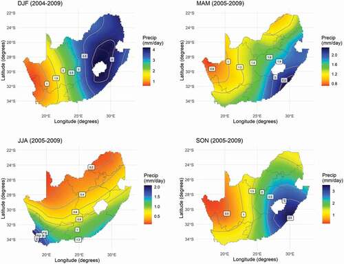
A 5-year mean seasonal climatology of rainfall spatial distributions was produced from monthly rainfall reanalysis data from Global Precipitation Climatology Project (GPCP). The GPCP is part of the Global Energy and Water Cycle Exchanges (GEWEX) activity under the World Climate Research Programme (WCRP). It provides a consistent long-term monthly analysis product of global precipitation from the integration of various satellite data sets of lands and oceans and a gauge analysis over land. The global merged data set has a spatial resolution of 2.5° latitude × 2.5° longitude grid, covering the period 1979–present. The data undergo a series of quality control procedures which include; assessing data against station meta-information (especially location), checking for coding, typing or transmission errors, automated checks that compares individual data for spatial homogeneity and climatological normal, flagging of questionable data after assessing orographic conditions and catalogues of catastrophic events, and calibration of satellites instruments against gauge data (Adler et al., 2018; Adler et al., 2003; Huffman et al., 1997). The data set is made available by the NOAA/ESRL: PSD through the website http://www.esrl.noaa.gov/psd/. The Geographic Information System (GIS) was used to plot all 5-year seasonal spatial distribution maps; for austral summer (DJF) 2004–2009, autumn (MAM) 2005–2009, winter (JJA) 2005–2009, and spring (SON) 2005–2009 seasons. The seasonal mean data at different locations was mapped and the spatial data gaps were completed by statistical interpolation method kriging.

3. Results

3.1 Surface meteorology analysis

Figure 2 shows the mean seasonal circulation patterns over Southern Africa, the South Atlantic, and Indian Ocean at the 1000 hPa pressure levels during 2004–2009. During the summer season the central interior of South Africa was dominated by the by a continental trough, indicated by low geopotential height values and was also flanked by anticyclone systems at the South Atlantic, and Indian Ocean, indicated by the high geopotential height values. The convergence of tropical and subtropical air masses driven by the surface trough and ridging Indian Ocean anticyclone, result in the uplifting of moist air and subsequently rainfall (Jury & Nkosi, 2000; Tyson et al., 1996). Figure 3 shows that the summer season is receiving the most seasonal rainfall and is disproportionately dominant on the eastern half of the country. During autumn, this 1000 hPa level continental trough moved northward as it was dislodged by the stability inducing ridging South Atlantic and Indian Ocean anticyclone. Figure 3 shows a generally reduced rainfall over the country during the autumn season and the maximum being confined along the east coast of the country. The geopotential height values in central interior of South Africa reached a maximum during winter, as the continental anticyclone is the dominant circulation system during this season (Garstang et al., 1996; Swap & Tyson, 1999; Tyson et al., 1996). During winter, the low values of the geopotential height in the mid-latitudes extended northward to the southern part of South Africa, indicating the transient mid-latitude convective westerly wave impacting the southern parts of South Africa (Freiman & Piketh, 2003). These westerly waves are associated with frontal system; they bring about on-shore flow of clean moist maritime air from South Atlantic and the Southern Oceans (Garstang et al., 1996; Ncipha et al., 2020; Swap & Tyson, 1999; Tyson et al., 1996). Figure 3 shows rainfall was dominant from the southwest coast and extending along the south coast to the east coast, the interior of the country was generally dry. During spring, the continental trough moved southward to the centre of the subcontinent, pushing the South Atlantic and Indian Ocean anticyclones out of the subcontinent. This displacement is indicated by the development of low geopotential height values at the centre of the subcontinent and the development of high geopotential height values southwest and southeast of the subcontinent. Figure 3 shows the CT study area is dry during spring while rainfall is disproportionally received over the eastern coast, as the result of the southward movement of the continental trough and ridging South Indian Ocean anticyclone (Figure 2).

Figure 2. Composite mean seasonal geopotential height (m) over Southern Africa, South Atlantic, and Indian Ocean at 1000 hPa pressure level during 2004–2009 period. Constructed from NCEP and NCAR reanalysis data.

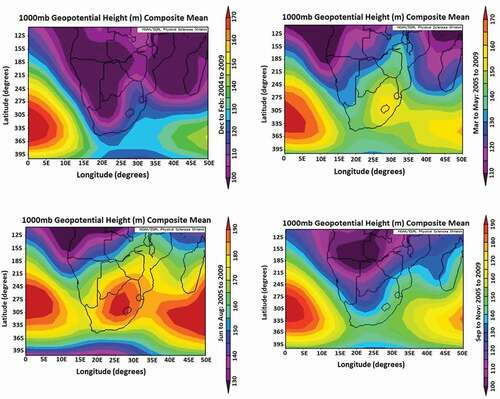
Figure 3. Composite mean seasonal daily rainfall (mm/day) over Southern Africa, South Atlantic, and Indian Ocean at 1000 hPa pressure level during 2004–2009 period. Constructed from NCEP and NCAR reanalysis data.

3.2 CO₂ seasonal surface spatial distribution in South Africa

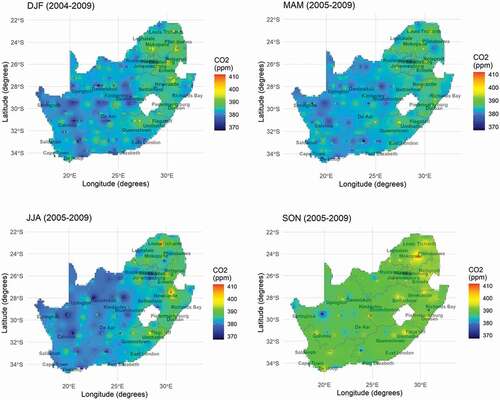
Figure 4 shows the seasonal surface spatial distribution of CO₂ in South Africa. The signatures of hotspots (areas of high CO₂ concentrations) were prevalent in the L, IHV, and KZN study areas in all seasons. The CO₂ loading at the hotspots is higher in winter and spring and the CO₂ signature patterns are spatially expanded in the two dry seasons of the interior of the country. There was a surprise consistent signature in all seasons, which occurred north of the EC study area, outside all selected study areas. As high concentrations were expected within the selected study regions known to be industrialized. This signature coincided with the fire incidence signature from year 2000 to 2008 (Forsyth et al., 2010).

Figure 4. Seasonal CO₂ surface spatial distribution in South Africa.

3.3 Annual variation of surface CO₂ loading at the study areas

Figure 5 shows the annual variation of surface CO₂ loading from 2005 to 2009 at the CT, NC, FS, EC, KZN, IHV, and L study areas, respectively. The slopes (R²) of the trend lines from simple linear regression analysis at all the study areas are positive, implying the surface levels of CO₂ at the study areas have been increasing (based on the satellite data with its associated uncertainties) during the period of analysis. Table 2 provides a list of the values of the CO₂ growth rate over years at all the study areas.

Figure 5. Monthly variation of surface CO₂ loading from December 2004 to December 2009 at CT, NC, FS, EC, KZN, IHV, and L, respectively.

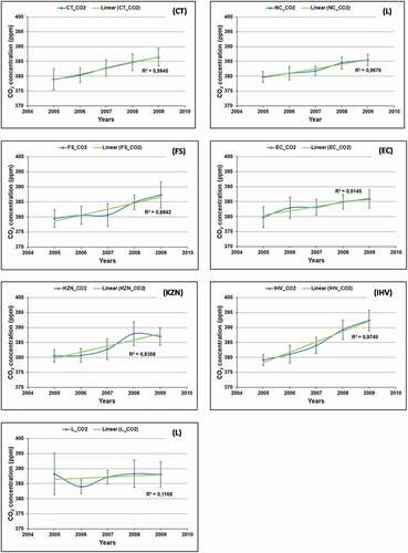
Table 2. CO₂ annual growth rate at the study areas

Area	ppm/yr
Cape Town (CT)	0.9945
Central Freestate (FS)	0.8842
Central Northern Cape (NC)	0.9676
Coastal Eastern Cape (EC)	0.9145
Coastal KwaZulu-Natal (KZN)	0.8358
Industrial Highveld (IHV)	0.9749
Limpopo (L)	0.1168

4. Discussions

The seasonal cycle of the emission strength of South Africa’s CO₂ sources determine the seasonal atmospheric CO₂ loading and its varied spatial distribution over the country (DEA, 2014; Diab et al., 2004; Osman et al., 2014; Silva et al., 2003). The national surface CO₂ foot print in South Africa resembles the spatial industrial CO₂ inventory established by Osman et al. (2014), especially during the summer and autumn seasons when the background loading in surface CO₂ is relatively low (Figure 2). During these two seasons the impact of point source industrial CO₂ emission stands out, as there are several occurrences of localized high surface CO₂ concentration places surrounded by large areas of low background concentrations.

The CO₂ loading at the hotspots is higher in winter and spring and the CO₂ signature patterns are spatially expanded in the two dry seasons (Figure 4), as a result of combined contributions of emissions from industries, domestic fossil fuel burning and biomass combustion (Diab et al., 2004; Silva et al., 2003). These wide CO₂ signatures are prevalent in the northeast and eastern part of the country particularly during the spring season. This is the result of the spatial and temporal variation of biomass burning in South Africa, with low occurrence in the semiarid western part of the interior (NC) of the country (Bond et al., 2003; Silva et al., 2003) and peak occurrence in September (Silva et al., 2003).

The seasonal spatial pattern of surface CO₂ atmospheric loading is also influenced by prevailing meteorology, which influences transport and mixing (Garstang et al., 1996; Swap & Tyson, 1999; Tyson et al., 1996). The CO₂ hotspots over the northeast and eastern part of the country stand out throughout all seasons. However, their spatial extent grew from summer to spring. During the summer season the central interior of South Africa was dominated by the convective and rain bearing continental trough (Figure 2). The low background concentrations during the summer season are due to moist unstable atmospheric conditions that are suitable for rapid pollution dispersion, mixing, and deposition by rainfall (Tyson et al., 1996) and carbon uptake by forests and savannas through photosynthesis (Fang et al., 2014; Valentini et al., 2014). In contrast, the CT study area was dominated by the off-shore flow during the summer season (Ncipha et al., 2020), driven by the ridging South Atlantic Ocean anticyclone (Figure 2), resulting warm and dry conditions along the southwest coast of the CT study area (Reason, 2017; Shikwambana et al., 2019). Causing a conducive condition for the development and spread of biomass fires along the southwest coast. Figure 3 shows the southwest coast of South Africa received the least rainfall during the summer season. As a result, there were some signatures of high CO₂ along the southwest coast of the CT study site (Figure 4). Ncipha et al. (2020) found that the summer surface average CO₂ concentration at the CT study area was not a seasonal minimum.

During the autumn season the background concentration of CO₂ started to increase together with the CO₂ hotspots spatial extents (Figure 4). As the continental trough was shifted northwards and displaced by the ridging South Atlantic and Indian Ocean anticyclones (Figure 2).

During the winter season, the CO₂ concentration of the hotspots was further increased together with their spatial extent signature and the general background levels of CO₂. However, there was a general reduction in the CO₂ background levels in the southwest and central interior part of the country (Figure 4). This is due to the prevalence of the passage of the westerly wave over the southern part of South Africa (Figure 2), which bring on-shore flow of clean maritime air from South Atlantic and the Southern Oceans. This air transport is usually accompanied by precipitation (Garstang et al., 1996; Ncipha et al., 2020; Swap & Tyson, 1999; Tyson et al., 1996). Figure 2 also shows a continental anticyclone system centred over the central part of the interior of South Africa. This anticyclone transports the emissions from the interior of the country to their exit over the east coast (Diab et al., 2004; Garstang et al., 1996; Ncipha et al., 2020; Tyson et al., 1996). Ncipha et al. (2020) found the surface CO₂ loading at the KZN and EC study sites to be a seasonal maximum during winter season.

During the spring season the CO₂ hotspots spatial extent was further increased and background levels reached maximum (Figure 4). This seasonal maximum was mainly driven by peak biomass fires emissions in spring (Silva et al., 2003). Figure 4 shows the NC study area had the most occurrences of low CO₂ spots during the spring season. This could be due to the area being semiarid and sparsely vegetated area (Bond et al., 2003; Silva et al., 2003). As a result relatively less biomass burning occurs there in comparison to the other areas (Bond et al., 2003; Silva et al., 2003). Ncipha et al. (2020) found the surface average CO₂ concentration over CT study area during spring was a seasonal maximum and the followed by summer. The warm and dry off-shore flow over the CT driven by the ridging South Atlantic anticyclone (Figure 2) is responsible for both these high seasonal CO₂ levels at CT study site (Figure 4).

The annual surface CO₂ levels have been increasing at the study sites during the study period. The CT area had the greatest growth, followed by IHV, NC, EC, FS, KZN, and L. The growth of the surface CO₂ concentration at the L study area was the smallest. However, the general surface loading of CO₂ in this area is the highest throughout the period of analysis. The growth rate of CO₂ at all the study sites is below the global growth rate (background stations), which was reported to be 2 ppm yr⁻¹ from 2007 to 2008 (WMO, 2009), and 1.6 ppm yr⁻¹ from 2008 to 2009 (WMO, 2010). The Cape point GAW station reported the growth rate (background air) of CO₂ to be varying between 1.6 and 2.1 ppm yr⁻¹ from 1993 to 2008 (Brunke et al., 2011; Labuschagne et al., 2018). Labuschagne et al. (2017) determined a growth rate of 0.77 ppm yr⁻¹ from 1993 to 2016 for continental-urban (non-background) air reaching the Cape Point GAW station. This growth rate is comparable to the ones determined at the study sites, except at L.

5. Conclusions

This study highlighted the importance of satellite data as an important tool in air quality management. TES CO₂ data provided for the first time a seasonal national spatial view of CO₂ distribution and its temporal variation in inadequately monitored South Africa, a dominant continental source region of fossil fuel CO₂ emissions.

This study demonstrated that the seasonal CO₂ atmospheric loading in South Africa is dependent on the seasonal cycle of emissions strength and meteorology.

The surface CO₂ foot print in South Africa resembles the industrial CO₂ emission sources spatial distribution, especially during the summer and autumn seasons when the background CO₂ surface loading is relatively low. During the two seasons, the impact of point sources industrial CO₂ emissions stands out.

In winter and spring seasons the surface CO₂ foot prints are spatially expanded as a result of contributions of emissions from biomass and domestic fossil fuel combustion. The wide CO₂ signatures are prevalent in the northeast and eastern part of South Africa particularly in the spring season, as a result of the spatial and temporal variation of biomass burning in Southern Africa.

All CO₂ hotspots were in the selected study sites that were based on the known national industrial CO₂ emissions inventory. However, there was a surprise seasonal consistent CO₂ signature that was outside the selected study regions. This signature was located just north of the EC study site.

The surface levels of CO₂ at the study areas have been increasing during the period of analysis. The CT area had the greatest growth, followed by IHV, NC, EC, FS, KZN and L. The growth of the surface CO₂ concentration at the L study area was the smallest, however the general surface loading of CO₂ in this area was the highest throughout the period of analysis. The growth rates at the study sites are comparable to the one from Cape Point GAW stations determined for continental-urban (non-background) air.

This study provides a baseline in terms of atmospheric spatial distribution of CO₂ and its temporal variation in South Africa. The large spatial coverage of satellite data is its strength over surface observational networks, particularly in an inadequately monitored region like South Africa. The study period extent was limited by the availability of complete or adequate recent data retrievals for the purpose of these analyses. Another important limitation to this study was the inherent nature of the monitoring platform being an orbital satellite. Orbital satellites are unable to provide high temporal resolution data as a result daily evolution of pollutants loading is not possible. A future study is planned to build on the established understanding of atmospheric CO₂ loading in South Africa using the latest available satellites data.

Disclosure of potential conflicts of interest

No potential conflict of interest was reported by the author(s).

Acknowledgments

We would like to thank the University of KwaZulu-Natal, School of Chemistry and Physics, Bureau Océan Indien of the Agence Universataire de la Francophonie (AUF), and the South African Weather Service for supporting this research work. We gratefully acknowledge the NASA Langley Research Centre for making the TES/Aura CO₂ data available online. We gratefully acknowledge NCEP, NCAR, and NOAA/ESRL: PSD for providing the reanalysis data and plots. Daulphin Razafipahatelo is acknowledged for guidance in developing MATLAB scripts for data analysis, Oupa Malahlela is acknowledged for improving the quality of geopotential heights maps plots.

References

- Adler, R. F., Huffman, G. J., Chang, A., Ferraro, R., Xie, P., Janowiak, J., Rudolf, B., Schneider, U., Curtis, S., Bolvin, D., Gruber, A., Susskind, J., Arkin, P., & Nelkin, E. (2003). The version-2 precipitation climatology project (GPCP) monthly precipitation analysis (1979-Present). Journal of Hydrometeorology, 4(6), 1147–1167. https://doi.org/https://doi.org/10.1175/1525-7541(2003)004<1147:TVGPCP>2.0.CO;2
- Adler, R. F., Sapiano, M., Huffman, G. J., Wang, -J.-J., Gu, G., Bolvin, D., Chiu, L., Schneider, U., Becker, A., Nelkin, E., Xie, P., Ferraro, R., & Shin, D.-B. (2018). The Global Precipitation Climatology Project (GPCP) monthly analysis (New Version 2.3) and a review of 2017 global precipitation. Atmosphere, 9(4), 138. https://doi.org/https://doi.org/10.3390/atmos9040138
- Beer, R. (2006). TES on the aura mission: Scientific objectives, measurements, and analysis overview. IEEE Transactions on Geoscience and Remote Sensing, 44(5), 1102–1105. https://doi.org/https://doi.org/10.1109/TGRS.2005.863716
- Beer, R., Glavich, T. A., & Rider, D. M. (2001). Tropospheric emission spectrometer for the Earth Observing System’s Aura satellite. Applied Optics, 40(15), 2358–2367. https://doi.org/https://doi.org/10.1364/AO.40.002356
- Bond, W. J., Midgely, G. F., & Woodward, F. I. (2003). What controls South African vegetation – Climate or fire? South African Journal of Botany, 69(1), 79–91. https://doi.org/https://doi.org/10.1016/S0254-6299(15)30362-8
- Brailsford, G. W., Stephens, B. B., Gomez, A. J., Riedel, K., Mikaloff Fletcher, S. E., Nichol, S. E., & Manning, M. R. (2012). Long-term continuous atmospheric CO2 measurements at Baring Head, New Zealand. Atmospheric Measurements Techniques, 5(12), 3109–3117. https://doi.org/https://doi.org/10.5194/amt-5-3109-2012
- Brunke, E.-G., Labuschagne, C., Parker, B., & Scheel, H. E., (2011). Recent results from measurements of CO2, CH4, CO and N2O at the GAW station Cape Point, 15th WMO/IAEA Meeting of experts on Carbon Dioxide, Other Greenhouse Gases and Related Tracers Measurement Techniques, Jena Germany, 7-10 September 2009.
- Canadell, J. G., Le Quéré, C., Raupach, M. R., Field, C. B., Bultenhuls, E. T., Clals, P., Conway, T. J., Gillett, N. P., Houghton, R. A., & Marland, G. (2007). Contributions to accelerating atmospheric CO2 growth from economic activity, carbon intensity, and efficiency of natural sinks. Proceedings of the National Academy of Sciences, 104(47), 18866–18870. https://doi.org/https://doi.org/10.1073/pnas.0702737104
- Department of Environmental Affairs. (2012). The highveld priority area air quality baseline assessment report 2010. Department of Environmental Affairs, ISBN978-0-621-39698-0.
- Department of Environmental Affairs, (2014). Greenhouse gas inventory South Africa 2000-2010. Retrieved October 07, 2020, from https://www.environment.gov.za/sites/default/files/docs/greenhousegas_invetorysouthafrica.pdf
- Deutscher, N. M., Sherlock, V., Mikaloff Fletcher, S. E., Griffith, D. W. T., Notholt, J., Macatangay, R., Connor, B. J., Robinson, J., Shiona, H., Velazco, V. A., Wang, Y., Wennberg, P. O., & Wunch, D. (2014). Drivers of column-average CO2 variability at Southern hemispheric total carbon column observing network sites. Atmospheric Chemistry and Physics, 14(18), 9883–9901. https://doi.org/https://doi.org/10.5194/acp-14-9883-2014
- Diab, R. D., Thompson, A. M., Mari, K., Ramsay, L., & Coetzee, G. J. R. (2004). Tropospheric ozone climatology over Irene, South Africa from 1990-1994 and 1998-2002. Journal of Geophysical Research, 109(D20), 301. https://doi.org/https://doi.org/10.129/2004JD004293
- Eskom. (2015). Map of eskom power stations. Retrieved October 07, 2020, from http://www.eskom.co.za/Whatweredoing/ElectricityGeneration/PowerStations/Pages/Map_Of_Eskom_Power_Stations.aspx
- Fang, S. X., Zhou, L. X., Tans, P. P., Ciais, P., Steinbacher, M., Xu, L., & Luan, T. (2014). In situ measurement of atmospheric CO2 at the four WMO/GAW stations in China. Atmospheric Chemistry and Physics, 14(5), 2541–2554. https://doi.org/https://doi.org/10.5194/acp-14-2541-2014
- Feig, G. T., Joubert, W. R., Mudau, A. R., & Monteiro, P. M. S. (2017). South African carbon observations. CO2 measurements for land, atmosphere and ocean. South African Journal of Science, 113(11/12), 1–4. https://doi.org/https://doi.org/10.17159/sajs.2017/a0237
- Forster, P., Ramaswamy, V., Artaxo, P., Berntsen, T., Betts, R., Fahey, D. W., Haywood, J., Lean, J., Lowe, D. C., Myhre, G., Nganga, J., Prinn, R., Raga, G., Schulz, M., & Van Dorland, R. (2007). Changes in Atmospheric constituents and in radiative forcing. In S. Solomon, D. Qin, M. Manning, Z. Chen, M. Marquis, K. B. Averyt, M. Tignor, & H. L. Miller (Eds.), Change 2007: The physical science basis. contribution of working group I to the fourth assessment report of the intergovernmental panel on climate change. (pp. 130–234). Cambridge University Press.
- Forsyth, G. G., Krugger, F. J. K., & Le Maitre, D. C., (2010). National veldfire risk assessment: Analysis of exposure of social, economic and environmental assests to veldfire hazards in South Africa. CSIR Report No: CSIR/NRE/ECO/ER/2010/0023/C, Council for Scientific and Industrial Research (CSIR). Retrieved October 08, 2020, from https://www.nda.agric.za/doaDev/sideMenu/ForestryWeb/webapp/Documents/Veldfire_Risk_Report_v11.pdf
- Freiman, M. T., & Piketh, S. J. (2003). Air transport into and out of the industrial Highveld region of South Africa. Journal of Applied Meteorology, 42(7), 994–1002. https://doi.org/https://doi.org/10.1175/1520-0450(2003)042<0994:ATIAOO>2.0.CO;2
- Garstang, M., Tyson, P. D., Swap, R., Edwards, M., Kållberg, P., & Lindesay, J. A. (1996). Horizontal and vertical transport of air over southern Africa. Journal of Geophysical Research, 101(D19), 23,721–23,736. https://doi.org/https://doi.org/10.1029/95JD00844
- Gimond, M. (2020). Intro to GIS and Spatial Analysis. Retrieved October 11, 2020, from https://mgimond.github.io/Spatial/index.html
- Huffman, G. J., Adler, R. F., Arkin, P., Chang, A., Ferraro, R., Gruber, A., Janowiak, J., McNab, A., Rudolf, B., & Schneider, U. (1997). The global precipitation climatology project (GPCP) combined precipitation dataset. Bulletin of the Americam Meteorological Society, 78(1), 5–20. https://doi.org/https://doi.org/10.1175/1520-0477(1997)078<0005:TGPCPG>2.0.CO;2
- Intergovernmental Panel on Climate Change, (1996). Report. In climate change 1995. The science of climate change, contribution of working group I to the second assessment report of the intergovernmental panel on climate change (IPCC). Cambridge University Press.
- Jones, D. B. A., Bowman, K. W., Logan, J. A., Heald, C. L., Liu, J., Lou, M., Worden, J., & Drummond, J. (2009). The zonal structure of tropical O3 and CO as observed by the tropospheric emission spectrometer in november 2004 – Part 1: Inverse modeling of CO emissions. Atmospheric Chemistry and Physics, 9(11), 3547–3562. https://doi.org/https://doi.org/10.5194/acp-9-3547-2009
- Jones, D. B. A., Bowman, K. W., Palmer, P. I., Worden, J. R., Jacob, D. J., Hoffman, R. N., Bey, I., & Yantosca, R. M. (2003). Potential of observations from the Tropospheric Emission Spectrometer to constrain continental sources of carbon monoxide. Journal of Geophysical Research, 108(D24), 4789. https://doi.org/https://doi.org/10.1029/2003JD003702
- Jury, M. R., & Nkosi, S. E. (2000). Easterly flow in the tropical Indian Ocean and climate variability over south-east Africa. WATER SA, 26(2), 147–152. http://wrcwebsite.azurewebsites.net/wp-content/uploads/mdocs/WaterSA_2000_02_1306.pdf
- Kulawik, S.S., Worden, J.R., Wofsy, S.C., Biraud, S.C., Nassar, R., Jones, D.B.A., Olsen, E.T., Jimenez, R., Park, S., Santoni, G.W., Daube, B. C., Pittman, J. V., Stephens, B. B., Kort, E. A., Osterman, G. B., TES team, (2013). Comparisons of improved Aura Tropospheric Emission Spectrometer CO2 with HIPPO and SGB aircraft profile measurements, Atmospheric Chemistry and Physics, 13, 3205–3225.
- Labuschagne, C., Joubert, W., Martin, L., Mkololo, T., Coetzee, T., Mbambalala, E., & vdSpuy, D., (2017, August 27-31). Recent updates from the Cape Point long-term data records, Poster presentation; 19th WMO/IAEA Meeting on Carbon Dioxide, Other Greenhouse Gases, and Related Measurement Techniques (GGMT-2017), (pp. 59), Empa Dübendof, Switzerland, Retrieved October 08, 2020, from https://www.empa.ch/documents/518954/1343679/P59_GGMT-2017.pdf/4c419028-6a4c-4c25-a761-ca523ddf5cc3
- Labuschagne, C., Kuyper, B., Brunke, E.-G., Mokolo, T., Van Der Spuy, D., Martin, L., Mbambalala, E., Parker, B., Khan, M. A. H., Davies-Coleman, M. T., Shallcross, D. E., & Joubert, W. (2018). A review of four decades of atmospheric trace gas measurements at Cape Point, South Africa. Transactions of the Royal Society of South Africa, 73(2), 113–132. https://doi.org/https://doi.org/10.1080/0035919X.2018.1477854
- Le Quéré, C., Raupach, M. R., Canadell, J. G., Marland, G., Bopp, L., Ciais, P., Conway, T. J., Doney, S. C., Feely, R. A., Foster, P., Friedlingstein, P., Gurney, K., Houghton, R. A., House, J. I., Huntingford, C., Levy, P. E., Lomas, M. R., Majkut, J., Metzl, N., Ometto, J. P., … Woodward, F. I. (2009). Trends in the sources and sinks of carbon dioxide. Nature Geoscience, 2(12), 831–836. https://doi.org/https://doi.org/10.1038/ngeo689
- Limpopo: Department of Economic Development, Environment & Tourism. (2013). ‘Provincial air quality management plan’. Retrieved October 08, 2020, from https://saaqis.environment.gov.za/documents/AQPlanning/LIMPOPO%20PROVINCIAL%20AQMP.pdf
- Morgan, E. J., Lavrič, J. V., Seifert, T., Chicoine, T., Day, A., Gomez, J., Logan, R., Sack, J., Shuuya, T., Uushona, E. G., Vincent, K., Schultz, U., Brunke, E.-G., Labuschagne, C., Thompson, R. L., Schmidt, S., Manning, A. C., & Heimann, M. (2015). Continuous measurements of greenhouse gases and atmospheric oxygen at the Namib Desert Atmospheric Observatory. Atmospheric Measurement Techniques, 8(6), 2233–2250. https://doi.org/https://doi.org/10.5194/amt-8-2233-2015
- National Oceanic and Atmospheric Administration, Carbon dioxide levels hit record peak in May. NOAA RESEARCH NEWS. National Oceanic and Atmospheric Administration (NOAA). Retrieved September 19, 2020, from https://research.noaa.gov/article/ArtMID/587/ArticleID/2461/Carbon-dioxide-levels-hit-record-peak-in-May
- Ncipha, X. G., Sivakumar, V., & Mahlalela, O. E. (2020). The influence of meteorology and air transport on CO2 atmospheric distribution over South Africa. Atmosphere, 11(287), 1–25. https://doi.org/https://doi.org/10.3390/atmos11030287
- Nickless, A., Ziehn, T., Rayner, P. J., Scholes, R. J., & Engelbrecht, F. (2015). Greenhouse gas network design using backward Lagrangian particle dispersion model – Part 2: Sensitivity analyses and South African test case. Atmospheric Chemistry and Physics, 15(4), 2051–2069. https://doi.org/https://doi.org/10.5194/acp-15-2051-2015
- Osman, K., Coquelet, C., & Ramjugernath, D. (2014). Review of carbon dioxide capture and storage with relevance to the South African power sector. South African Journal of Science, 110(5/6), 1–12. Art.#2013-0188. Retrieved October 08, 2020, from https://doi.org/https://doi.org/10.1590/sajs.2014/20130188
- Puukka, J., Dubarle, P., McKiernan, H., Reddy, J., & Wade, P., (2012). Higher education in regional and citydevelopment: The free state,South Africa, Organisation for economic co-operation and development. Organisation for Economic Co-operation and Development (OECD). Retrieved October 08, 2020, from http://www.oecd.org/education/imhe/50008631.pdf
- Reason, C. J. C. (2017). Climate of Southern Africa. In Hans von Storch (Ed.), Oxford research encyclopedia of climate science. Oxford University PressPublisher. doi:https://doi.org/10.1093/acrefore/9780190228620.013.513
- Rinsland, C. P., Luo, M., Logan, J. A., Beer, R., Worden, H., Kulawik, S. S., Rider, D., Osternman, G., Gunson, M., Eldering, A., Goldman, A., Sherphard, M., Clough, S. A., Rodgers, C., Lampel, M., & Chiou, L. (2006). Nadir measurements of carbon monoxide distribution by the Tropospheric Emission Spectrometer instrument onboard the Aura Spacecraft: Overview of analysis approach and examples of initial results. Geophysical Research Letters, 33(L22806), 1–6. https://doi.org/https://doi.org/10.1029/2006GL027000
- Sabine, C. L., Feely, R. A., Gruber, N., Key, R. M., Lee, K., Bullister, J. L., Wanninkhof, R., Wong, C. S., Wallace, D. W. R., Tilbrook, B., Millero, F. J., Peng, T.-H., Kozyr, A., Ono, T., & Rios, A. F. (2004). The oceanic sink for anthropogenic CO2. Science, 305(5682), 367–371. https://doi.org/https://doi.org/10.1126/science.1097403
- Schoeberl, M. R., Douglass, A. R., Hilsenrath, E., Bhartia, P. K., Waters, J. W., Gunson, M. R., Froidevaux, L., Gille, J. C., Barnett, J. J., Levelt, P. F., & DeCola, P. (2006). Overview of the EOS aura mission. IEEE Transactions on Geosciences and Remote Sensing, 44(5), 1066–1074. https://doi.org/https://doi.org/10.1109/TGRS.2005.861950
- Shikwambana, L., Ncipha, X., Malahlela, O. E., Mbatha, N., & Sivakumar, V. (2019). Characterisation of aerosol constituents from wildfires using satellites and model data: A case study in Knysna, South Africa. International Journal of Remote Sensing, 40(12), 4743–4761. https://doi.org/https://doi.org/10.1080/01431161.2019.1573338
- Silva, J. M. N., Pereira, J. M. C., Cabral, A. I., Sá, A. C. L., Vasconcelos, M. J. P., Mota, B., & Grégoire, J. (2003). An estimate of the area burned in southern Africa during the 2000 dry season using SPOT-VEGETATION satellite data. Journal of Geophysical Research, 108(D13), 8498. https://doi.org/https://doi.org/10.1029/2002JD002320
- South African Government. (2015). South Africa’s provinces. Retrieved October 08, 2020, from http://www.gov.za/about-sa/south-africas-provinces
- Swap, R. J., & Tyson, P. D. (1999). Stable discontinuities as determinants of the vertical distribution of aerosols and trace gases in the atmosphere. South African Journal of Science, 95(2), 63–70. https://www.researchgate.net/publication/261706848_Stable_discontinuities_as_determinants_of_the_vertical_distribution_of_aerosols_and_trace_gases_in_the_atmosphere
- Tyson, P. D., Garstang, M., Swap, R., Kållberg, P., & Edwards, M. (1996). An air transport climatology for subtropical southern Africa. International Journal of Climatology, 16(3), 265–291. https://doi.org/https://doi.org/10.1002/(SICI)1097-0088(199603)16:3<265::AID-JOC8>3.0.CO;2-M
- United Nations Development Programme. (2016). The integrated fire management handbook: Establishing fire protection associations in South Africa. Retrieved October 08, 2020, from http://fynbosfire.org.za/development/wp-content/uploads/2015/02/A-Guide-to-IFM_Complete_Display.pdf
- Valentini, R., Arneth, A., Bombelli, A., Castaldi, S., Cazzolla Gatti, R., Chevallier, F., Ciais, P., Grieco, E., Hartmann, J., Henry, M., Houghton, R. A., Jung, M., Kutsch, W. L., Malhi, Y., Mayorga, E., Merbold, L., Murray-Tortarolo, G., Papale, D., Peylin, P., Poulter, B., … Scholes, R. J. (2014). A full greenhouse gases budget of Africa: Synthesis, uncertainties, and vulnerabilities. Biogeosciences, 11(2), 381–407. https://doi.org/https://doi.org/10.5194/bg-11-381-2014
- Western Cape: Department of Environmental Affairs and Development. (2017). Western cape state of air quality management report 2017. Retrieved October 08, 2020, from https://www.westerncape.gov.za/eadp/files/atoms/files/SoAR_2017_1.pdf
- Williams, C. A., Hanan, N. P., Neff, J. C., Scholes, J. R., Berry, J. A., Denning, A. S., & Baker, D. F. (2007). Africa and the global carbon cycle. Carbon Balance and Management, 2(3), 1–13. https://doi.org/https://doi.org/10.1186/1750-0680-2-3
- Worden, J., Kulawik, S. S., Shephard, M. W., Clough, S. A., Worden, H., Bowman, K., & Goldman, A. (2004). Predicted errors of tropospheric emission spectrometer nadir retrievals from spectral window selection. Journal of Geophysical Research, 109(D09308), 1–12. https://doi.org/https://doi.org/10.1029/2004JD004522
- World Meteorological Organisation. (2010). ‘The state of greenhouse gases in the atmosphere based on global observations through 2009ʹ. WMO Greenhouse Gas Bulletin, 6, 1–4. Retrieved October 08, 2020, from https://library.wmo.int/index.php?lvl=notice_display&id=13802
- World Meteorological Organisation. (2012). ‘The state of greenhouse gases in the atmosphere based on global observations through 2011ʹ. WMO Greenhouse Gas Bulletin, 8, 1–4. ISSN 2078-0796. Retrieved October 08, 2020, from https://library.wmo.int/index.php?lvl=notice_display&id=13804
- World Meteorological Organisation. (2013). ‘The state of greenhouse gases in the atmosphere using global observations through 2012ʹ. WMO Greenhouse Gas Bulletin, 9. Retrieved October 08, 2020, from https://library.wmo.int/index.php?lvl=notice_display&id=15864
- World Meteorological Organisation. (2014). ‘The state of greenhouse gases in the atmosphere using global observations through 2013ʹ. WMO Greenhouse Gas Bulletin, 10, 1–8. ISSN 2078-0796. Retrieved October 08, 2020, from https://library.wmo.int/index.php?lvl=notice_display&id=16396
- World Meteorological Organisation. (2018). The state of greenhouse gases in the atmosphere based on global observations through 2017. WMO GHG Bulletin, 14, 1–8. ISSN 2078-0796. Retrieved October 08, 2020, from https://library.wmo.int/doc_num.php?explnum_id=5455
- World Meteorological Organization. (2009). The state of greenhouse gases in the atmosphere based on global observations through 2008. WMO Greenhouse Gas Bulletin, 5, 1–4. Retrieved October 08, 2020, from https://library.wmo.int/index.php?lvl=notice_display&id=14759