School effectiveness in Zambia: The origins of differences between rural and urban outcomes

Abstract

Surveys have shown that Zambian urban residents have significantly higher schooling attainment rates than rural residents and are more likely to be literate. To address this inequality in education outcomes it is important to understand to what extent this is a result of a resource gap (for example, differences in teachers or textbooks) or different returns on resources (for example, an additional teacher makes more of a difference in urban areas). To explore this idea this study performed an Oaxaca decomposition on the SACMEQ II data set for Zambia. The results showed that the rural–urban gap was attributable both to differences in the presence of resources (55% of the gap) and differences in the returns on resources (45% of the gap). Since returns on resources are considerably lower in rural areas, additional resource investment alone is unlikely to close the gap between rural and urban schooling outcomes.

Keywords:

• education outcomes
• rural schools
• Zambia

JEL codes:

• I21
• O55

1. Introduction

The education system in Zambia is notorious for its geographical inequities. Surveys have shown that urban residents have significantly higher educational attainment than rural residents and are considerably more likely to be literate (Burger et al., 2004). The average educational attainment of Zambians is much higher now than it was four decades ago, but the large geographical gaps in educational attainment have remained. The implied inequities in access to education and quality of education are unfair because they may prevent young people from gaining the knowledge and qualifications required to pursue opportunities and realise their dreams. In addition to being unfair, the urban bias in the allocation of education is also expected to be inefficient on a macroeconomic level, because it hampers the optimal allocation of resources.

Cross-tabulations of survey data reveal that a child in a city or town is likely to have access to better teachers, more teaching resources and a family environment that places a higher premium on schooling. In addition to having access to more and higher quality resources, there is reason to suspect that the returns to resources may be higher in an urban environment, where systems often run more smoothly because of, among other things, the superior infrastructure and more frequent monitoring.

Using the Southern Africa Consortium for Monitoring Educational Quality (SACMEQ) II data set on Zambia, this paper explores the extent to which the existing urban bias in schooling outcomes can be attributed to differences in resources vis-à-vis differences in the efficient use of resources. This question is of pivotal importance for educational policy making in Zambia because such analysis will indicate how best to address the current geographical gap in educational outcomes. If this gap is largely attributable to differences in resources between rural and urban schools, the government will have to concentrate on increasing rural access to resources. If, however, the gap is mostly due to differences in the efficient use of resources, then investment in additional resources alone is unlikely to have the desired effect.

Reading test scores were selected as the indicator of schooling outcomes because of their widespread use as a measure of education and human development. A school-level model was estimated because the focus of the paper is on policy making and impediments to service delivery.

The rest of this paper is divided into four sections. Section 2 briefly describes the data, delineating the differences between rural and urban aggregates for test scores, as well as school resource and socioeconomic variables. Section 3 explains the model's specification and the reasons for using it. Section 4 estimates, assesses and interprets the school-level model. It describes the Oaxaca decomposition that was performed on the estimated model to investigate how the contribution of resources compares with the contribution of the efficient use of resources to the observed gap between rural and urban schooling outcomes. Section 5 concludes and offers recommendations.

2. Data and descriptive analysis

The paper uses the International Institute of Educational Planning's SACMEQ II data set for Zambia. The data were collected in 2000, using three questionnaires: for pupils, for teachers, and for school heads.

The survey sample was stratified according to the nine Zambian regions, and in each of these the school sample was selected to be representative of different school sizes. The total sample includes 2611 pupils and 173 schools. The survey targeted Grade 6 classes, so most of the information captured in the pupil and teacher questionnaires pertains only to this grade.

The SACMEQ data sets are rich in many dimensions. The availability of a teacher quality variable – based on a test administered to teachers – is possibly their most alluring feature. They also allow a more nuanced analysis of geographical factors. Instead of the traditional binary rural–urban indicator, the SACMEQ data set for Zambia contains a four-category school location indicator, identifying isolated areas, rural areas, small towns and large cities. At the pupil level, there are 64 observations for isolated schools, 1308 for rural schools, 474 for schools in small towns and 696 for schools in large towns or cities. However, for the school level the present study reverts to the traditional rural–urban categories (classifying isolated and rural schools as rural and the rest as urban) because the sample contains only five schools in the isolated areas and because the differences between the small and large towns in Zambia are often not large or interesting enough to justify this distinction. There were 93 schools in rural areas, 30 schools in small towns and 41 schools in large towns or cities.

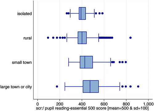
Cross-tabulations of the SACMEQ II data set show clear evidence of urban bias, not only in schooling outcomes but also, as would be expected, in resources and inputs. The box-and-whisker plot in Figure 1 illustrates the differences in mean values as well as variations by location of school. Pupils at schools in isolated areas scored an average of 402.3 on the literacy test, while those at schools in rural areas scored an average of 411.1 for the same test. In small town schools, the average pupil score was 445.2, while in large towns and cities it was 482.5. The variance patterns also differed by region: there was considerably more variation in test scores in urban and semi-urban areas. For instance, the coefficient of variation was 0.21 for large towns or cities but 0.16 for isolated areas. The lower variation in isolated and rural areas compared with small and large towns can be interpreted as evidence of greater constraints on learning in isolated and rural areas. Similar patterns were observed for mathematics test results.

Figure 1: Literacy test scores by school location

The differences in school outcomes by location can also be seen in Table 1, which tabulates grade repetition by school location. Of pupils in urban schools, 56% had never repeated a grade, while for pupils in rural schools this figure was 40%. The hypothesis of independence of the two variables was rejected at a 1% significance level.

Table 1: Frequency of grades repeated, by school location

	Rural	Urban
0	40%	56%
1	44%	31%
2	12%	6%
3	3%	7%
Total	100%	100%

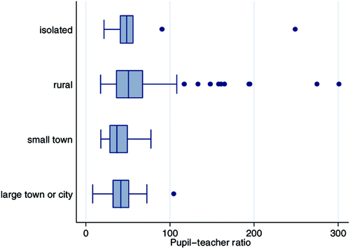
It was expected that if much of the gap in rural–urban performance was due to resource differences, there would also be large discrepancies in rural–urban resource levels. This hypothesis is investigated in the rest of this section. As expected, the data suggest that there is a significant difference between rural and urban resources. The average pupil–teacher ratio was 64.8 for rural areas, 41.2 for small towns and 42.6 for large towns and cities. Analysis of variation shows that the hypothesis of equal means was rejected at the 1% significance level. The box-and-whisker plot in Figure 2 shows that there were noticeably more instances of extremely high pupil–teacher ratios (between 80 and 300) in schools located in isolated and rural areas. Of the 13 schools with pupil–teacher ratios of 100 and above, 12 were rural schools.

Figure 2: Pupil–teacher ratios by school location

There also appeared to be evidence of considerable differences in teacher effort. Table 2 reports the shares of no homework given and the frequency with which children reported that their homework was corrected. The hypothesis of independence was rejected at the 1% significance level.

Table 2: Frequency of homework corrected in English class, by school location

	Rural	Urban
No homework given	34%	29%
Homework never corrected	7%	4%
Homework sometimes corrected	25%	22%
Homework corrected most of the time	17%	19%
Homework always corrected	15%	26%
Total	100%	100%

Surprisingly, the survey shows that pupils in rural schools were significantly more likely to have good access to a textbook (own book or share with only one other pupil) than pupils in urban schools. Also contrary to what one might expect, there were no significant urban–rural differences in any of the indicators of teacher quality.

Urban schools were more likely to be regularly subjected to full inspections. Table 3 shows that 57% of rural schools but only 40% of urban schools had not had a full inspection in the previous two years. The hypothesis of independence of the two variables was rejected at the 1% level of significance.

Table 3: Full inspection of school in past two years, by school location

	Rural	Urban
No full inspection	57%	40%
Full inspection	43%	60%
Total	100%	100%

Table 4: Going without meals, by school location

	Rural	Urban
Pupil does not normally miss any meals in a week	43%	65%
Pupil normally misses at least one meal a week	57%	35%
Total	100%	100%

Table 5: Frequency of receiving help with homework, by school location

	Rural	Urban
No homework	3%	1%
Never	19%	13%
Sometimes	56%	61%
Most of the time	22%	25%
Total	100%	100%

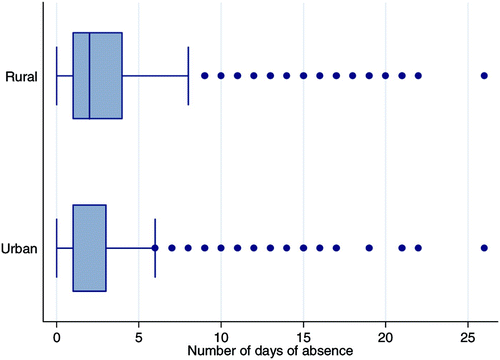
There are also indications that the demand for education may have been lower in rural areas. According to the survey, rural schools had a higher incidence of pupil absenteeism and more pupils starting school over-age. The survey showed that more than 41% of pupils in rural schools were over-aged, while less than 15% of pupils in urban schools were over-aged. Figure 3 shows that pupils in rural schools were more likely to stay away from school. The average number of self-reported days of absence during the previous month was 2.2 for pupils in urban schools and 2.9 for pupils in rural schools. The hypothesis of an equal mean was rejected at a 1% significance level. It was also interesting to see that for pupils in rural schools the dispersion of observations above the mean was wider than the dispersion of observations for pupils in urban schools. Not only was the expected number of days of absence higher in rural areas, there was also a greater likelihood of being absent from school for six days or more.

Figure 3: Pupil absenteeism by school location

Relating to the higher poverty and lower levels of education in rural areas, the data show that rural pupils were also less likely to receive assistance with homework, and there were fewer books in the homes of pupils attending rural schools.

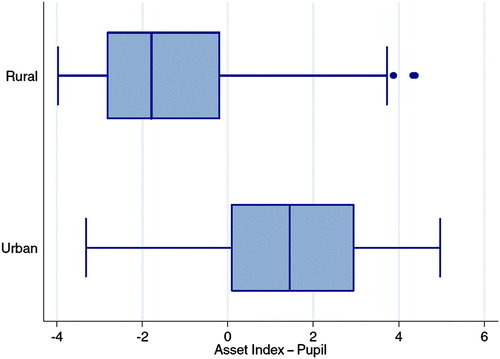
The SACMEQ II survey has no information on income or expenditure, so, following Sahn and Stifel (2000) and Asselin (2002), an asset index was constructed to provide an indication of household income. Principal components analysis was used to determine the weights of the variables in the index. The variables used for constructing the index and the assigned weights are listed in Appendix A. A higher score on the asset index shows that a household had more possessions, which was interpreted as an indication of a higher socioeconomic status. The index shows large discrepancies between the average bundle of assets possessed by the households of pupils in rural schools and that possessed by households of pupils in urban schools. The rural mean asset index score was –1.28, while the urban score was 1.33. The hypothesis of equal means for the asset indices of the two school locations was rejected. Figure 4 shows the distribution of the asset index by school location. If the bundle of assets used to compile the asset index was not sufficiently broad, asset indices could fail to capture rural wealth adequately. It was thus encouraging to see that there were pupils in rural schools whose households were ranked among the most affluent according to the asset index scores.

Figure 4: Asset index by school location

Figure 5: Years of education of pupils' mothers, by school location

Figure 6: Parental assistance index by school location

Table 4 shows that the proportion of pupils reporting regularly going without a meal also differed significantly by school location. Of those in rural schools, 57% claimed that they regularly missed at least one meal a week, whereas only 35% of urban pupils usually missed one or more meal a week.

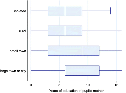
The survey also indicated that education levels were lower in more isolated and rural areas. The mean number of years of education for pupils' mothers was 6.0 for pupils in schools in isolated areas, 6.6 years for pupils in rural schools, 8.0 years for pupils in schools in small towns and 9.9 years for pupils in schools in large towns and cities. The hypothesis of equal means was rejected at the 1% level of significance. The same pattern also holds for the medians of these groups.

Furthermore, Table 5 indicates that pupils in rural schools reported receiving less regular help with their homework (from a person other than their teacher). As would be expected, this variable was not independent of the pupil's mother's education. Pupils who claimed that they never received help with their homework had mothers with a mean education level of 6.7 years, while those who received help with their homework most of the time had mothers with a level of 8.6 years. The hypothesis of equal means was rejected at the 1% level. Clearly, pupils with less educated mothers were at a disadvantage compared to those with more educated mothers and, because mothers' education levels were considerably lower in rural areas (Figure 5), this effect reinforced the urban advantage in schooling outcomes.

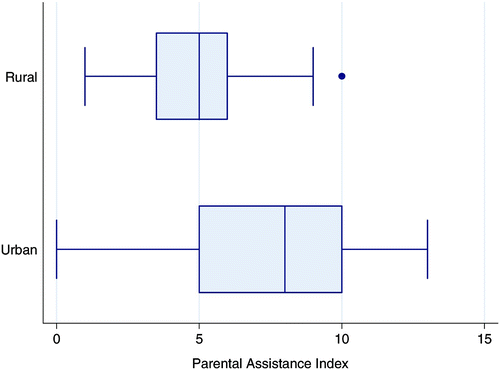
It appears that mothers' education had an impact on schooling outcomes not only because of the level of assistance provided to their children but also because of the level of assistance provided to the school. The average education of pupils' mothers (for the surveyed pupils in Grade 6) and the assistance offered by parents (as reported by the school head)1 had a strongly significant and positive correlation. There were also geographical patterns in the level of parental assistance provided (Figure 6). Even when controlling for mothers' education, an urban dummy remained a highly significant explanatory variable for parental assistance. Regression analysis showed that location had an impact on the level of parental assistance that stretched beyond its correlation with mothers' education.

The SACMEQ data did not report travel time to school for pupils. The Demographic and Health Survey EdData Survey 2002 is an alternative school survey conducted at roughly the same time that did capture this information. According to the summary report (Central Statistical Office, Zambia & ORC Macro [CSO & ORC], 2003), the distance from home to the closest school was considerably further for rural residents. For their sample of 8027 children between the ages of 6 and 14, the average walking time to school was 15 minutes for urban residents and 41 minutes for rural residents. For 14% of rural residents, the walking time to the closest school exceeded an hour, while this was the case for less than 1% of urban residents.

The EdData survey report (CSO & ORC, 2003) also contained information on how many pupils had dropped out of school or never attended school and what motivated these decisions. For the combined sample of individuals between ages 5 and 24, 38.1% of those in the lowest household wealth quintile had never attended school, while this was the case for only 11.3% of those in the top wealth quintile. The percentage of respondents (aged between 5 and 24) in urban areas who had never attended school was 17.4% in urban areas, but 31.4% in rural areas.

The survey estimated that by Grade 6, 14.4% and 21.7% of the Grade 1 class in urban and rural schools respectively would have dropped out. Costs were most often cited by parents as the reason for deciding to remove a child from school (58.9%). The child no longer wanting to attend school and the distance to school were the reasons for dropping out in 11.9% and 11.7% respectively of the cases recorded.

3. Model specification

The central research question for this study concerned the relative contribution of resources and returns on resources to education outcomes. This research is thus situated within the contours of the theoretical and empirical literature on school effectiveness and specifically the economics literature on education production functions. Hence it assumes that education is produced using a number of measurable inputs such as the pupil's ability and effort, the pupil's socioeconomic background, and the quality and quantity of teachers, textbooks and classrooms.

The pitfalls of the restrictive assumptions of the production function approach are widely acknowledged. Many critics object in principle to borrowing concepts and techniques from manufacturing to understand and elucidate the education process, because these processes are clearly worlds apart. Other criticisms are more technical and relate to the rigid model specification and the associated implicit assumption that the education process – as it plays out in various schools and for various individuals – is similar enough to be comparable. Additionally, it is not clear that the most important inputs in the education process can be standardised and captured accurately. The influence of teachers is a good example: it is viewed as a key input, but the standard measurable proxies for teachers, such as teacher-pupil ratio, teacher qualifications, teacher test scores and teacher salary, are not robustly significant and are regarded as poor approximations of the influence of teachers on pupils (Hanushek, 2008).

Many of the other criticisms are more generic, relating to statistical problems often encountered with regression analysis. For instance, because many of the most important influences are so difficult to capture and measure, there is also scope for considerable omitted variable bias. Additionally, the simple one-equation specification of the traditional education production function cannot reflect the complicated interactions between the inputs and outcomes, which can introduce simultaneity bias.

Despite these criticisms, however, the education production function has remained popular in the empirical literature on education and policy debates. Part of its appeal is no doubt the simplicity of the approach and its intuitive interpretation. But its enduring popularity may also be partly attributable to a lack of more attractive alternatives. Hanushek (1979) argues that many alternative methods do far worse. Studies that observe the impact of one input in depth – but in isolation – are generally far less useful for policy discussions than a comparison of the impact of key resources. Also, Hanushek (1979) points out that the aspects of the education process that are measurable are often also the aspects that are most easily replicable and it is thus appropriate that these should be the focus of the empirical analysis.

Although production functions were originally conceived to describe manufacturing processes, education production functions have strayed from their roots and are now implemented according to a conceptual framework that is far removed from the initial theories. For instance, it is seen as unrealistic to assume that schools lie on the so-called production possibility frontier (a theoretical representation associated with optimality and efficiency). According to Bowles (1970), decision makers in the field of education possess neither the information nor the systemic understanding required to ensure optimisation. Furthermore, they are constrained by many legal and political factors. Hanushek (1979) adds that these decision makers are not motivated to pursue maximum outcomes or to minimise costs and inputs. Because inputs may not always be used to their full potential, coefficients should be interpreted as marginal effects at average levels. For this reason it is important to consider the differences in the productivity not only of a variety of inputs but also of a particular input across schools or groups of pupils or regions.

Schooling outcomes or quality are viewed as the result of the weighted sum of a series of inputs:

y = β ₁ F + β ₂ S + β ₃ A + μ

Here y represents the performance of the school, F is the inputs relating to the social environment (including the socioeconomic background of the pupils), S represents school inputs, A is the individual characteristics of the schools' pupils (including innate ability and pupil motivation), and is an error term.

On the basis of the large observed rural–urban gaps in the availability and quality of resources, the initial hypothesis was that most of the variation between rural and urban test scores was attributable to differences in resources The aim was to test this hypothesis by estimating a parsimonious model that would be valid for both rural and urban schools and that would capture the main determinants of education quality.

The model for schooling outcomes was estimated at the school level, so pupil inputs and family inputs were aggregated per school. Average per school scores on a reading test represented the quality of the schools' outcomes. Between-school variance accounted for 30% of the overall variation in the SACMEQ II reading test scores. Differences between rural and urban schools were responsible for 45% of the between-school variances.

While aggregating to the school-level may introduce aggregation bias which could inflate the estimated impact of resources (see Hanushek et al., 1996), it avoids the measurement error associated with using school-wide variables to explain pupil-level effects. Hanushek et al. (1996) also maintain that the impact of omitted variable bias can be reduced when estimation is done on a level where there are fewer missing variables. It can thus be argued that the decision to focus on the school level may reduce the omitted variable bias attributable to the exclusion of measures for ability in the regression.

There are at least two likely sources of bias relating to this omission. Firstly, as discussed in the previous section, a substantial proportion of children never enter school and, according to the DHS EdData 2002 survey report (CSO & ORC, 2003), the likelihood of never entering school was considerably higher among children of rural residents and poor households. Also, according to the DHS EdData survey, a much higher proportion of rural pupils had dropped out by Grade 6. It was not possible to test or correct for selection bias within this survey because there was no information available in the survey on children of the same age group who were not attending school. However, the literature suggests that pupils who drop out or never attend school are likely to have lower ability on average (Glewwe & Jacoby, 1994),2 and we have seen that these problems were more prevalent and occurred earlier in the rural parts of Zambia. Thus we would expect the bias operating via this relationship would result in an underestimation of the size of the urban–rural gap.

Secondly, there is a positive effect operating via school choice, which is expected to work in the opposite direction. Where there is a choice of schools, it can be argued that good schools would often attract children who are more able. Given that the literature and the descriptive analysis appear to indicate that there is a higher concentration of good schools in urban areas, this can introduce a positive bias, inflating the urban–rural gap.

This source of bias is more of a concern than the drop-out rate, as it may lead us to be overly bold in our findings and our recommendations. However, while we are aware of this problem, we do not consider the scale of the problem to be such that it prohibits undertaking the analysis. This effect is expected to be weaker in a country such as Zambia where school choice may be less prevalent because cost is such a prominent consideration in schooling decisions and geographical mobility is constrained. The higher rural incidence of pupils never attending school or dropping out is expected to result in a negative bias and will thus work against the bias introduced via the school choice effect.

Multicollinearity is also a concern in education production functions. Although it does not introduce systematic bias, the associated inflation of the standard errors can contaminate the coefficients and destabilise the model, which is, of course, problematic if the coefficients are to be used for policy analysis. In this paper the problem is addressed by orthogonalising variables.

4. Comparing rural and urban schools

Prior to testing, variables were orthogonalised using a modified Gram–Schmidt procedure (in the order in which the variables are listed in Table 6). Reported coefficients relate to the original variable values and were retrieved after estimation by reversing the orthogonalisation. To avoid heteroscedasticity, the p-values in Table 6 were based on robust Hubert–White standard errors.

Table 6: Impact of resources on schools

	Full sample		Sample of urban schools		Sample of rural schools
	Coefficient	p-value	Coefficient	p-value	Coefficient	p-value
Average years of education for parents	4.74	0	8.25	0	2.97	0
Asset index	9.19	0	3.96	0.01	5.16	0.01
Pupil–teacher ratio for school	–0.05	0.04	–0.58	0.05	–0.06	0.04
Proportion of pupils who speak English frequently	49.6	0	105.86	0	35.85	0
Constant	355.88	0	303.14	0	372.4	0
R-squared	0.48		0.38		0.26
Sample size	169		71		98

Although the four-variable model is simple, it is credible. It includes the most important dimensions of education performance from the literature. More complex specifications failed to explain more of the variance. Other candidate variables from the literature such as teacher quality indicators, access to textbooks, school infrastructure and equipment did not enter the models significantly and also did not affect the coefficients of these variables. The parsimonious model appeared to be remarkably stable and robust. It includes the following four variables:

•	Two of the four significant regressors – the average asset index and the average parental educational attainment – were interpreted as representing mainly the influence of socioeconomic status and household circumstances, which would be classified as family inputs according to the theoretical model. The analysis in Section 2 showed that parental education had a significant relationship with both the level of parental assistance provided to the schools and the proportion of pupils receiving help with their homework. Parental education was calculated using the highest parental educational attainment.
•	The pupil–teacher ratio is a vital school input.
•	The proportion of pupils who spoke English frequently was viewed as a critical individual-level input, capturing exposure to and confidence with the use of the language of instruction.

Given its parsimony, the full sample model performed well. With its four variables, the model managed to explain 48% of the variance between schools. Appendix B shows histograms of the errors, and Appendix C shows the predicted test score averages for schools compared with the actual scores.

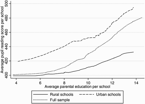
The average number of years of education for parents was strongly significant. These models suggested that parental education had a higher yield in terms of school performance in urban areas. The regression coefficients indicated that raising the average parental educational attainment by one year is expected to raise the average school test score by 8.3 marks in urban schools and 3.0 marks in rural schools. The flatness in the rural school coefficient was not due to a lack of variation in the average parental education level. There were nine rural schools where the average parental education level exceeded 12 years. Figure 7 is a Lowess smoothing graph depicting the relationship between the school averages for parental education and the pupils' reading scores. The graph illustrates the geographical discrepancies in the impact of parental education on school performance for the overlapping distribution (the region where we can reliably compare urban and rural schools), without controlling for other factors. The locally weighted regression line for urban schools lies above the line for the full sample, and the full sample line is above the line for rural schools. The graph suggests that a rural school was expected to perform worse than an urban school with the same level of parental educational attainment.

Figure 7: Parental education and average pupil reading test scores

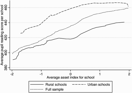
The asset index is interpreted as an indicator of socioeconomic status. Contrary to what we find for the other resources, the regression predicted that an increase in socioeconomic status (as approximated by the asset index) would have a bigger impact on school performance in the rural areas. All other things being equal, a unit increase in the average asset index for a school would have raised a school's average reading test score by more than 5 points in rural areas and almost 4 points in urban areas. The Lowess graph in Figure 8 shows that urban schools outperformed rural schools where students had the same socioeconomic profile.

Figure 8: Asset index and average pupil reading test scores

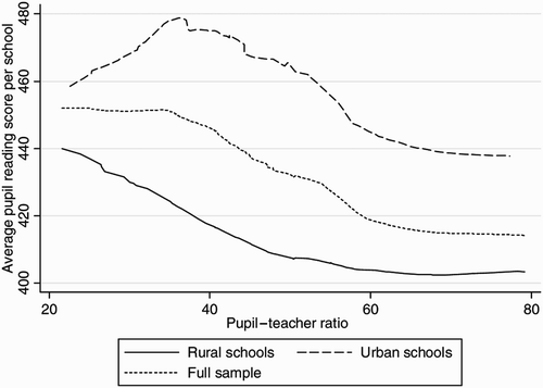
The pupil–teacher ratio had a negative and strongly significant relationship with the school's average reading test score. The regression coefficient was larger in urban areas than in rural areas, suggesting a higher yield in terms of school performance resulting from additional teachers in urban areas. The Lowess curve in Figure 9 plots the relationship between school test scores and pupil–teacher ratio and at the same pupil–teacher ratios urban schools tend to perform better than rural schools.

Figure 9: Pupil–teacher ratio and average pupil reading test scores

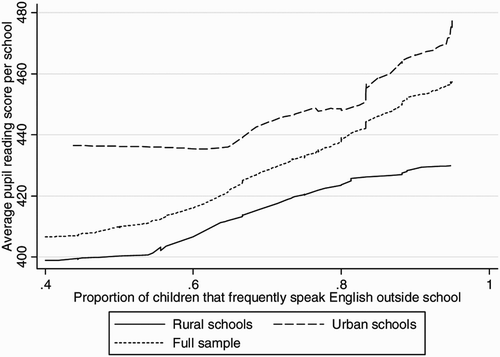
The proportion of pupils who reported speaking English regularly outside school had a strongly positive relationship with school outcomes. The coefficient was 105.9 for urban schools and 35.9 for rural schools; thus, according to the regression, all other things being equal, a 10 percentage point increase in the proportion of pupils who spoke English frequently is expected to result in an 11-point rise in the average reading test score of an urban school and a four-point rise in a rural school's score. The graph in Figure 10 shows that – without controlling for other variables – urban schools would have done better than rural schools with the same proportion of pupils who spoke English frequently.

Figure 10: Proportion regularly speaking English outside school and average pupil reading test scores

To compare the influence of the four determinants in the model, the regression coefficient could be multiplied by the variable's standard deviation to calculate the impact of one standard deviation change on school outcomes. According to Table 7, the proportion of pupils who spoke English frequently had the highest average impact for both the urban and rural school models.

Table 7: Impact of one standard deviation change on school outcomes

	Full sample			Sample of urban schools			Sample of rural schools
	Coefficient	Standard deviation	Estimated average impact	Coefficient	Standard deviation	Estimated average impact	Coefficient	Standard deviation	Estimated average impact
Average years of education for parents	4.74	2.31	10.95	8.25	1.91	15.76	2.97	2.21	6.56
Asset index	9.19	1.9	17.46	3.96	1.59	6.30	5.16	1.15	5.93
Pupil–teacher ratio for school	–0.05	42.4	–2.12	–0.58	41.94	–24.33	–0.06	51.57	–3.09
Proportion of pupils who speak English frequently	49.6	0.28	13.89	105.86	0.15	15.88	35.85	0.3	10.76

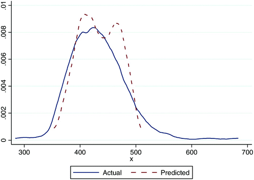
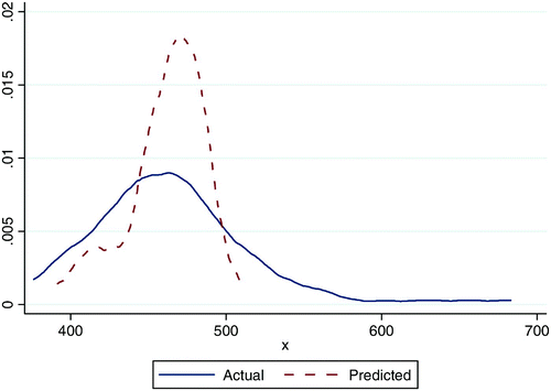
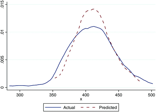
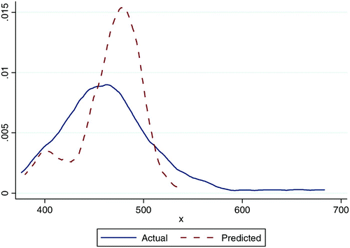
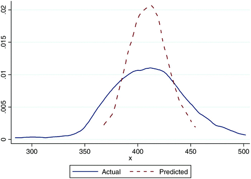
Table 8 decomposes the rural–urban gap in the schools' average test scores for reading. The models for urban and rural schools were used to generate predicted values. The average predicted urban school test score was 465, while the average predicted rural test score was 410. The Oaxaca decomposition used these two numbers to calculate the size of the rural–urban gap. There was a 56-point gap between the average predicted values of rural and urban schools.

The method attributed the gap to two potential sources: a difference in resources and a difference in the returns on resources. To distinguish these two sources, the rural schools model was applied to the urban schools data to estimate how schools with an urban profile would have performed in rural conditions. When the rural schools model was used to predict test scores for the sample of urban schools, the average test score was 441. The difference between the average test score for schools with urban levels of resources operating in rural conditions (441) and schools with urban levels of resources operating in urban conditions (468) reflects the estimated point difference that can be attributed to a difference in the returns on inputs. The remainder of the rural–urban gap in test scores, which was 31 points and represented 55% of the gap, was ascribed to differences in the schools' inputs and resources.

Table 8: Oaxaca decomposition of the rural–urban gap in school outcomes

	Test score
Average test score for schools with rural levels of resources in rural circumstances	409.79
Average test score for schools with urban levels of resources in rural circumstances	440.55
Average test score for schools with urban levels of resources in urban circumstances	465.44
	Test score	Percentage
Rural–urban gap in test score	55.65	12%
Rural–urban gap in test score attributed to differences in resources	30.76	55%
Rural–urban gap in test score attributed to differences in returns to resources	24.89	45%
Note: According to this method the rural–urban gap is defined as the difference between the predicted test scores of the urban schools according to a model of urban schools (i.e. urban resources and urban returns to resources) and the predicted test scores of rural schools based on a rural schools model (i.e. rural resources and rural returns to resources). This rural–urban gap is then decomposed to see how much of the gap can be attributed to differences in resources and how much to different rates of return to resources.

Although there were large gaps in the rural–urban levels of inputs for many vital determinants, resource differences alone explained just over half of the rural–urban gap in schooling outcomes. The rest of the gap was due to urban–rural differences in the relationship between the inputs and schooling outcomes. Schools in urban areas were not only in an advantaged position in terms of the quality and quantity of available inputs; they were also able to make better use of these inputs.

5. Conclusion

This study made it clear that there was a large discrepancy between the outcomes of rural and urban schools in Zambia. The analysis showed that this gap was attributable to both differences in resources (57% of the gap) and differences in the returns on resources (43% of the gap).

In research on development policies, it is customary to assume that there will be differences in the level of resources and the structure of relationships in rural and urban areas. For policy making, it can be vital to understand why there is a difference between rural and urban performance. Additional resource investment is unlikely to eliminate this gap if lower returns on inputs are responsible for a substantial proportion of the gap. Although additional resource investment will undoubtedly be a step in the right direction, resource investment will not have the required impact unless the efficiency gap is also addressed. Further investigation is required to provide a better understanding of the lower returns on school inputs in rural areas. Findings from previous studies would suggest that management skills and teacher motivation are important factors to consider.

Notes

¹This index was compiled by summing the number of ‘yes' answers to 14 questions about parents' contributions to school deliverables in the School Head questionnaire.

²Glewwe and Jacoby (1994) found that ability is a predictor of both late enrolment (negative correlation) and educational attainment (positive correlation).

Appendix A. Description of variables used to construct the asset index

Table A1: List of asset index variables and their assigned weights

Variable	Assigned weight
Does home where pupil stays have radio?	0.162
Does home where pupil stays have TV?	0.312
Does home where pupil stays have VCR?	0.178
Does home where pupil stays have telephone?	0.193
Does home where pupil stays have car?	0.141
Does home where pupil stays have piped water?	0.297
Does home where pupil stays have electricity?	0.312
Does pupil normally skip one or more meal a week?	-0.173
Is the floor of the home where pupil stays made mostly of earth or clay, or does it have no covering?	-0.336
Is the floor of the home where pupil stays made mostly of canvas?	-0.018
Is the floor of the home where pupil stays made mostly of wooden planks?	-0.009
Is the floor of the home where pupil stays made mostly of cement?	0.270
Is the floor of the home where pupil stays covered mostly with carpet or tiles?	0.112
Are the outside walls of the home where pupil stays made mostly of cardboard, plastic sheeting or canvas?	-0.021
Are the outside walls of the home where pupil stays made mostly of reeds, sticks or thatch grass?	-0.123
Are the outside walls of the home where pupil stays made mostly of stone or mud bricks?	-0.224
Are the outside walls of the home where pupil stays made mostly of metal sheets or asbestos sheets?	0.020
Are the outside walls of the home where pupil stays made mostly of wood?	-0.006
Are the outside walls of the home where pupil stays made mostly of cut stone, concrete blocks or burned bricks?	0.289
Is the roof of the home where pupil stays made mostly of cardboard, plastic sheeting or canvas?	-0.003
Is the roof of the home where pupil stays made mostly of thatch grass or mud?	-0.348
Is the roof of the home where pupil stays made mostly of metal sheets or asbestos sheets?	0.315
Is the roof the home where pupil stays made mostly of cement or concrete?	0.053
Is the roof of the home where pupil stays made mostly of tiles?	0.024

Appendix B. Histograms of errors for three models of school outcomes

Figure B1: Errors for school outcomes model for full sample

Figure B2: Errors for school outcomes model for urban schools

Figure B3: Errors for school outcomes model for rural schools

Appendix C. Kernel density curves comparing actual and predicted test scores

Figure C1: Actual and predicted test scores using school outcomes model for full sample

Figure C2: Actual and predicted urban test scores using school outcomes model for full sample

Figure C3: Actual and predicted rural school test scores using school outcomes model for full sample

Figure C4: Actual and predicted test scores using school outcomes model for urban schools (using urban schools model)

Figure C5: Actual and predicted test scores using school outcomes model for rural schools (using rural schools model)

References

- Asselin , L-M . 2002 . Multidimensional Poverty: Composite Indicator of Multidimensional Poverty , Québec : Institut de Mathématique Gauss, Lévis .
- Bowles , S . 1970 . “ Towards an educational production function ” . In Education, Income and Human Capital , Edited by: Hansen , W L . Cambridge, MA : National Bureau for Economics Research .
- Burger , R , Burger , R P and Van der Berg , S . 2004 . A note on trends in the Zambian labour market between 1991 and 1998 , Mimeo. A Background Paper for the World Bank .
- CSO & ORC (Central Statistical Office, Zambia, and ORC Macro) . 2003 . Zambia DHS EdData Survey 2002: Education Data for Decision-Making , Calverton, MD : Central Statistical Office and ORC Macro .
- Glewwe , P and Jacoby , H . 1994 . Student achievement and schooling choice in low-income countries . Journal of Human Development , 29 ( 3 ) : 834 – 64 .
- Hanushek , E A . 1979 . Conceptual and empirical issues in the estimation of educational production functions . Journal of Human Resources , 14 ( 3 ) : 351 – 88 .
- Hanushek , E A . 2008 . “ Education production functions ” . In Palgrave Dictionary of Economics. 2nd ed , Edited by: Durlauf , S N and Blume , L E . New York : Palgrave Macmillan .
- Hanushek , E A , Rivkin , S G and Taylor , L L . 1996 . Aggregation and the estimated effects of school resources . Review of Economics and Statistics , 78 ( 4 ) : 611 – 27 .
- Sahn , D E and Stifel , D C . 2000 . Poverty comparisons over time and across countries in Africa . World Development , 28 ( 12 ) : 2123 – 55 .