Nature and determinants of household retirement savings behaviour in South Africa

Abstract

This study investigates the savings behaviour among South African households using the General Household Survey data for the periods 2002–04 and 2008–10. The age-cohort analysis shows that households achieve their income peaks when the household heads are in their early forties, earlier than in most other countries. Although initial support for the life-cycle hypothesis framework in the form of smoothed consumption was found from multivariate analysis, a closer examination reveals that the consumption–income ratio is also smooth over the age and cohort variables. This indicates that savings rates do not follow a hump-shape pattern as required in the life-cycle hypothesis framework. While households are seen to be able to maintain their consumption in retirement years through government grants, a large portion of the grants seem to be utilised for savings. This shows that the government grants have the dual effect of sustaining consumption levels while disincentivising savings during working years.

Keywords:

• household savings
• life-cycle hypothesis
• global financial crisis
• South Africa

JEL codes:

• D14
• D31
• D91
• O55
• G01

1. Introduction

The household savings rate in South Africa is one of the lowest among the developing countries. While the household savings rate in 2010 stood at 25% and 28% for India and China respectively, South Africa had a rate of −0.8% (Reserve Bank of India, 2014; Wan, 2011; South African Reserve Bank, 2015). Even more worrying is that the South African rate has been declining over recent decades (Aron et al., 2007). This has implications for the future economic well-being of not only South African households but also the economy as a whole because it constrains economic growth through low levels of domestic investment and places excessive fiscal burden on the government to provide for the old. It is hence of importance to understand the nature and determinants of household savings in South Africa.

The objective of this study is to comprehend the household savings behaviour and assess whether the life-cycle hypothesis (LCH) applies in the South African context with a representative sample. This is especially relevant because government policies tabled by the South African National Treasury to encourage household savings are devised and formulated on the assumption that South African households follow the LCH (National Treasury of South Africa, 2012a, 2012b).

Section 2 of the paper reviews literature briefly. This is followed by Sections 3 and 4 that undertake data description and discussion on the methodology respectively. Section 5 presents the cohort analysis, followed by the econometric estimation in Section 6. Conclusions are then drawn in the final section.

2. Literature review

The theoretical literature suggests a variety of motives for household saving, most of which can be grouped into five broad categories, namely: to smooth consumption over the lifetime (life-cycle motive); to benefit from interest and asset appreciation (inter-temporal substitution motive); to bequeath an inheritance (bequest motive); to finance large expenditure such as a house or education (down-payment motive); and to finance unexpected losses of income (precautionary saving). Although diverse, these motives are often overlapping (Browning & Lusardi, 1996).

Economic theory on savings behaviour is closely related to the theory of consumption. Keynes (1936) sees current income as the main determinant of consumption and savings, with consumption increasing at a rate lower than the increase in income. This implies that an increase in income leads to increased savings, with savings rising faster than income. The LCH, on the contrary, considers consumption to be dependent on the agent's life resources. Modigliani (2005a) introduces age-related consumer heterogeneity to this paradigm, with the propensity to save differing across age and cohorts. According to this approach, households maximise the benefits of consumption over their lifetime, subject to the constraints of expected lifetime income and initial wealth. Rational agents do this by smoothing their consumption over their life-time. This implies that savings are expected to be negative in the early years of an individual's life but increase with working years until they peak, typically just before retirement. Thereafter, savings decline as retirement begins, creating the hump-shape of the LCH. The permanent income hypothesis (PIH) (Friedman, 1957) focuses on the consumption of an ‘infinitely-lived’ consumer where consumption is more a function of permanent income than current income. The deviation of the PIH from the LCH lies in the former considering savings to be the result of transitory income, which is defined as the difference between current and permanent income. The prediction, therefore, is that a temporary increase in income leads to an increase in savings while a permanent increase in income leads to a fall in current savings as consumers increase consumption in anticipation of future income. Consumption is considered to be smoother under the PIH and LCH as compared with Keynesian theory. The other similarity between the LCH and the PIH is that both consider the saving rate to be independent of the level of current income.

There has been an explosion of empirical work following the formulation of the LCH and its variants using both microeconomic and macroeconomic data in various country contexts (Modigliani, 1986, 2005a; Deaton, 1992; Browning & Crossley, 2001; Pistaferri, 2009; Belke et al., 2012). However, not all empirical investigations in various country contexts have concluded that the savings behaviour follow the LCH (Huang & Caliendo, 2011). Using micro data, Deaton (1992) comes down fairly strongly in favour of the proposition that consumption tracks income over the life cycle. Deaton & Paxson (1994) and Poterba (1994) find that old people save more than younger people or at least do not dissave as suggested by the LCH. Carroll & Summers (1991) finds that in a country like the USA with a low savings rate, consumption and income move together in the long run.

There are various reasons for this. Firstly, liquidity constraints resulting from low income levels and excessive consumption requirements during the earning period of life results in limited or no savings; and secondly, bequest motives do not lead to dissaving during retirement years. Rational household behaviour maximises utility over lifetime taking into consideration the transfer payments including old age pensions from the government. Uncertainty of life-span and non-insurable health hazards induce the elderly to hold assets for precautionary purposes, thus reducing the rate of wealth decumulation during retirement. Lastly, the costs associated with planning an optimal consumption-saving plan also contribute to its non-implementaton (Huang & Caliendo, 2011).

Most studies exploring the LCH and the determinants of household savings in South Africa have used macroeconomic data (Aron & Muellbauer, 2000, 2006; Prinsloo, 2000; Simleit et al., 2011; Mahlo, 2012). At the microeconomic level, studies mostly focus on specific population groups like the urban/rural poor, the black middle class and the health impacts of HIV/AIDS on savings behaviour in South Africa. Analysing the rural black households in South Africa, Spio & Groenewald (1996) conclude that the strong family ties which characterise most rural households make it unnecessary for young and middle-age households to save for future retirement. Esson (2003) found that, contrary to the expectations of the LCH, the retired household members residing in Khayelitsha/Mitchells Plain saved more than the younger members, primarily to finance the funeral costs. Studies focusing on the Black middle class (du Plessis, 2008; Chauke, 2011) found them to dissave and attributed this to a lack of self-control encouraged by the culture of consumerism and easier access to credit. Health issues such as HIV/AIDS and malaria are also found to severely affect saving behaviour due to losses in labour productivity, income, human capital building, increasing medical expenses, social costs, a decline in life expectancy, and funeral costs (Sachs & Malaney 2002; Freire, 2004a, 2004b, 2004c; Mba 2007).

Overall, micro-level household savings studies on South African households have been highly targeted, where conclusions could be reached only for specific population groups.

3. Data

The data employed for the study are derived from the General Household Surveys (GHSs) of 2002, 2004, 2008 and 2010. The GHS is conducted by Statistics South Africa and consists of individual data (categorised as person and worker files) and household data. The GHS does not usually track the same households over time, but the samples of 2002 and 2008 were repeated in 2004 and 2010 respectively providing us with two true panel sets. Hence, the study excluded the interim years and utilised the two two-period panel datasets for the study.

A comparison of the survey sample with the national population illustrates that the GHS is representative of the total population of South Africa (Tables 1, 2 and 3). Although the study acknowledges the availability of other datasets such as the National Income Dynamics Survey data, the GHS provides a greater number of years of household data.

Table 1: Population size (in millions)

	National	Weighted GHS	Weighted sample used in estimation
2002	45.81	45.45	3.57
2004	47.02	46.45	3.70
2008	49.56	48.66	4.99
2010	50.90	49.86	4.84

Source: Stats SA (2013).

Table 2: Male by age group (%)

	2002		2004		2008		2010
Age	National	Sample	National	Sample	National	Sample	National	Sample
15 to 19	16.6	0.7	16.3	0.8	15.2	2.7	14.5	3.4
20 to 24	15.4	1.2	15.5	0.8	15.6	1.3	15.4	1.0
25 to 29	13.5	7.3	13.5	6.4	14.2	5.3	14.5	3.9
30 to 34	11.3	11.9	11.5	11.5	11.7	10.8	12.0	9.5
35 to 39	9.5	14.8	9.5	11.8	9.6	12.7	9.8	10.5
40 to 44	8.4	15.1	8.1	14.4	7.8	12.2	7.8	12.1
45 to 49	7.3	12.5	7.1	11.8	6.8	13.2	6.7	13.7
50 to 54	6.0	10.9	5.9	11.8	5.9	11.8	5.9	12.6
55 to 59	4.7	7.6	4.7	9.2	4.8	10.2	4.8	10.7
60 to 64	3.2	7.5	3.4	8.4	3.6	8.1	3.7	9.0
65 to 69	2.2	4.8	2.3	6.7	2.4	5.9	2.4	6.4
70 to 74	1.3	3.7	1.4	4.3	1.6	3.6	1.7	4.8
75 to 79	0.7	2.0	0.9	2.2	0.9	2.3	0.9	2.4

Source: GHS sample calculations.

Table 3: Female by age group (%)

	2002		2004		2008		2010
Age	National	Sample	National	Sample	National	Sample	National	Sample
15 to 19	15.5	1.0	15.1	1.1	14.1	3.0	14.2	3.5
20 to 24	13.9	1.8	14.3	1.4	14.4	1.4	14.8	1.1
25 to 29	11.6	3.6	11.9	3.4	12.8	3.9	14.2	3.9
30 to 34	10.2	7.5	10.1	6.2	10.1	7.8	10.8	5.4
35 to 39	9.5	10.4	9.1	9.0	8.6	9.9	9.0	8.0
40 to 44	9.3	12.3	8.7	11.5	8.0	11.4	8.1	10.7
45 to 49	8.3	12.2	8.1	11.1	7.9	11.8	8.0	13.9
50 to 54	6.7	10.6	6.8	11.7	6.9	12.5	7.3	12.9
55 to 59	5.3	9.3	5.4	10.5	5.7	11.4	1.0	10.4
60 to 64	3.9	9.8	4.0	10.7	4.4	8.5	4.9	10.5
65 to 69	2.8	8.8	3.0	10.0	3.2	7.8	3.4	6.7
70 to 74	1.8	8.8	2.0	8.9	2.3	6.4	2.6	6.9
75 to 79	1.2	4.0	1.4	4.4	1.6	4.1	1.7	6.1

Source: GHS sample calculations.

However, the data source presented many challenges. GHS survey data are arranged in three separate files: person, worker and household. The creation of our dataset required merging data across these files and over the years and removing observations with inconsistencies.

The individual household responses to questions relating to age, gender, population group and education level did not always match over the two years in each of the panels. There were also missing data due to omissions. Problems further arose from the definition of the household; household heads residing in the same dwelling unit resulted in issues of multiple-headed households. The last point illustrates a limitation in the GHS methodology because a household is defined as a group of individuals living in the same dwelling unit, such as a residential house, and not by the composition of a (true) household.

In overcoming the issues in the data, person and worker files were firstly merged where the age, gender and population group of the individual that shared the same unique identifier were checked. The age of the individual was permitted to increase by one, two and three years in order to account for birthdays that were passed, still to come and that had arrived when the interview took place. All households with heads whose age, gender and population group did not match across the two files were dropped from the sample. Similarly, all persons with missing information on income and expenditure were also dropped.

If a household head's details differed across the two-year period, the change in marital status was first checked before excluding the household completely. The study allowed for changing household heads based on changes in marital status of the previous household head. This occurred when household heads were re/married, separated, divorced or widowed. The changing household compositions, and household size, were allowed in order to retain large sample sizes.

Limitations to income and expenditure data also required a sorting and cleaning process. Where information on total monthly income and expenditure of the household was given as interval data, the average of the bracket was taken. Where exact income values were provided, total household income was determined by summing up the earnings of all household members from salaries and wages, remittances, farm good sales, social grants and other. All income and expenditure amounts were annualised and accounted for taxes and tax thresholds specific to each year. All amounts were deflated to 2008 constant prices.

The biggest challenge of the dataset is the absence of savings and wealth data. The methodology used to derive the savings variable is described in detail in the next section. A proxy for wealth ownership was created from the ownership of physical assets such as a car and house. Since the value of the house and car were not given, the wealth proxy is included in the analysis as a dummy variable. This has the advantage, however, of lowering the possibility of endogeneity issues. Nevertheless, we account for the possibility of endogeneity by using an instrumental variable for the wealth variable in the two-stage least squares (2SLS) for estimation.

The final household sample available for analysis after cleaning and sorting of data is shown in Table 4.

Table 4: Number of households

	Number of households
	GHS	Estimation sample
2002	26 243	4 888
2004	26 204	4 888
2008	24 222	5 072
2010	25 548	5 072

Source: Stats SA (2002, 2004, 2008, 2010) and GHS sample calculations.

The sample composition of the two panels (2002–04 and 2008–10) shows consistency across the various demographic variables (Table 5). Changes in the composition of single-headed households (includes divorced, widowed and separated spouses) and dependence on pensions and grant incomes show increases over the years. Main income source, however, has shown a definite shift in the second period (2008–10) from salaries to non-regular income from remittances and sale of non-farm/farm goods. This is indicative of the economic slowdown experienced by the South African economy over 2009/10 (Verick, 2010).

Table 5: Comparison of demographics across the panel samples (%)

		Panel data				Pooled data
Categorical Variable	Description	2002	2004	2008	2010	2002, 2004, 2008, 2010
Gender	Male	59.5	59.49	53.96	53.96	56.52
	Female	40.49	40.5	46.03	46.03	43.48
Population group	African/black	74.54	74.51	82.04	82.03	78.56
	Non-African/non-black	25.46	25.49	17.96	17.97	21.44
Marital status	Single	42.73	43.66	41.84	49.87	44.63
	Married	57.27	56.34	58.16	50.13	55.37
Location	Urban	59.57	59.62	56.41	56.42	57.88
	Rural	40.43	40.38	43.59	43.58	42.12
Wealth	Own house and car	23.14	22.63	19.97	20.40	21.43
	Do not own house/car	76.86	77.37	80.03	73.21	76.85
Education	Tertiary level	11.64	11.97	10.38	6.52	10
	Non-tertiary level	88.36	88.03	89.62	93.48	90
Main income	Salaries and wages	54.09	50.31	51.63	44.18	49.89
	Pensions and grants	24.46	30.39	34.84	34.67	24.15
	Other: remittances, sale of non-farm/farm goods	21.45	19.30	13.53	21.15	25.96
Social grants	Recipients	5.44	28.80	29.08	32.13	25.38
	Non-recipients	94.56	71.20	70.92	67.87	75.62

Source: Stats SA (2002, 2004, 2008, 2010). Authors’ own calculations.

Table 6 shows that urban, male, married, non-black households are seen to have higher income and consumption levels as compared with rural, female, single, black households respectively. The data are largely in keeping with our expectations of the South African economy.

Table 6: Median household consumption, income and grants

	Total household consumption	C/Y ratio	Total household income	Social grants
Male	17 993.99	0.92	19 578.31	11 280
Female	10 834.34	0.96	11 280	11 280
Black	10 834.34	0.93	11 675.68	11 280
Non-black	40 534.96	1.12	36 145.33	341.11
Tertiary	61 467.26	0.83	74 016.39	0
Non-tertiary	10 834.34	0.93	11 675.68	11 280
Single	10 805.41	0.93	11 675.68	11 280
Married	17 993.99	1.01	17 759.56	1 054.21
Urban	17 993.99	0.91	19 879.52	11 280
Rural	10 805.41	0.96	11 280	11 280
Total	11 993.99	0.99	12 131.15	11 280

Source: Stats SA GHS (2002, 2004, 2008, 2010). Authors’ own calculations.

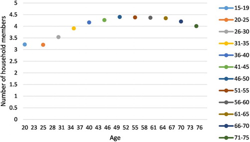
Household size across the age cohorts illustrates an increase in family size, peaking between the ages of 46 and 50 (Figure 1). On average, households consist of a minimum of three members, reaching a maximum of four and five until declining in the post-retirement ages of 71 to 75 years. This trend suggests that either children of the household do not leave until much later in life or that older household heads help out with caring for extended families and grandchildren (Duflo, 2003).

Figure 1: Mean household size

4. Methodology and estimation model

The methodology adopted is largely determined by the data at hand and taking cohort effects into account to control for possible inter-generational differences in income, attitudes and policies. Jappelli (1999) states that of the three ways to control for the presence of cohort effects – panel data, out-of-sample information, and repeated cross-sectional data – panel data are the most appropriate. We implement a two-pronged approach to understand the nature of savings behaviour by firstly undertaking an age-cohort graphical analysis of income, consumption and the marginal propensity to save based on repeated cross-sectional data; and secondly through an econometric analysis using panel data regressions (for the two panels 2002–04 and 2008–10) and pooled 2SLS to account for the endogeneity between wealth and consumption. A lagged wealth variable is used as the instrument for the wealth variable, reducing the dataset to pooled data covering 2004 and 2010.

The age-cohort technique is adapted from Deaton (1985). The steps involved are as follows: the household heads are classified under 12 cohort categories based on the birth year of the head of the household, and the means of income, consumption and propensity to save (using Equation (1)) are estimated for each category of cohort for each survey year. The LCH pattern is expected to be revealed through the hump-shape of income and marginal propensity to save and a smoothed out consumption pattern.

The marginal propensity to save is estimated over the age-cohort groups with the consumption function using repeated cross-sectional data:(1)

where β + γ is the marginal propensity to consume (MPC) and it follows that (1 – MPC) is the marginal propensity to save.

In our econometric approach, we estimate Equations (2) and (3) using pooled ordinary least squares (OLS), panel data and 2SLS techniques and derive implications regarding savings behaviour from them:(2) (3)

where ln C and ln C/Y are the log of household consumption and household consumption to income ratio respectively, LCH is a vector of age, age squared, income, wealth and grants, Demographics includes the household size, education, gender, marital status, location and ethnicity control, Cohorts are the dummies for the cohorts and Macro includes the interest rate and global financial crisis (GFC) dummy.

Lifetime resource theories of both the LCH and PIH emphasise the role of wealth in smoothing the consumption of an agent over his life-span. Increased saving in the earning years of life leads to accumulation of wealth, and sustaining consumption in the retirement years leads to erosion of wealth. Moreover, wealth in the form of a physical asset provides an agent with collateral to access the financial system. Hence wealth is expected to have a positive impact on consumption as well as the consumption–income ratio. The wealth dummy included takes the value one for households that own both a house and a car.

The LCH approach forecasts a smoothed consumption over the years of an agent's life where the life resources, rather than the income at the time of consumption, are its determinant. Controlling for age and cohort, higher income is expected to lead to an increase in consumption under the LCH. Increase in household income, however, is likely to be negatively related to the consumption–income ratio, indicating a higher saving rate at higher income levels.

Under the LCH, consumption is expected to be smoother than income over the life of the agent. This differs from the Keynesian approach, which expects age to display a non-linear (hump-shape) effect on consumption through the income effect. However, under the LCH the consumption–income ratio is expected to follow a U-shape over the life-span, which follows that the saving ratio would be hump-shaped.

Consumption differences between cohorts are expected to reflect the changes in the productivity and attitudes of generations over time. Eleven dummies are included to capture the 12 cohort categories, with Cohort 5 being taken as the benchmark category.

South Africa's unique social pension and grant system has the potential to distort household savings behaviour under the LCH framework because these transfers come to be perceived as regular income (Case & Deaton, 1998; Betrand et al., 2003; Esson, 2003; van der Berg et al., 2010). This is because transfer income, especially old age pension, can impact consumption levels at the older stage of life without eroding the wealth. Also, anticipation of such transfers can remove the compulsion to save during earning years, thus distorting the savings behaviour foreseen by the LCH. Total grants is hence expected to have a positive effect on consumption and a negative effect on the consumption–income ratio.

Finally, the demographic factors of a household – although not explicitly mentioned in Modigliani (2005a) framework – have been employed in the empirical analyses of household savings behaviour (Deaton & Paxson, 1994). Case & Deaton (1998) point out that differentiating based on population group is important to contribute to the understanding of South African household savings behaviour. A dummy (Black = 1 for black, and 0 otherwise) is included to capture the differences in the consumption behaviour between the majority population group of African/black households and the rest of the population. The consumption level and consumption–income ratio of households is expected to be positive for households with a married head (Single = 1 for unmarried/divorced, and 0 for married).

Households with a female head have been observed to have lower savings (Chowa, 2006), while the education levels of the head, which proxies for skills, has been observed to positively impact savings (Lusardi, 2007). Gender dummy included takes value 1 for females and 0 for males. Education dummy takes the value 1 for those with tertiary education and 0 for the rest. A dummy for location (Location = l for urban and 0 for rural) is included because urban households are expected to have both higher incomes and consumption levels.

The interest rate variable is included to account for the asset appreciation effect. An increase in interest rate is expected to decrease consumption both of savers as well as borrowers. The inter-temporal benefits to save increases with higher interest rates for borrowers and the cost of borrowing increases for those spending on credit. Lastly, a dummy is also included to capture the macroeconomic effects of the global financial crisis (GFC = 1 for the year 2010, and 0 otherwise), which potentially decreased the household's resources (Verick, 2010).

Table 7: Cross-section of age, cohorts and birth years

	2002/04			2008/10
1	2	3	4	5	6	7	8
Cohort: birth years	N	Age in 2002	Age in 2004	N	Age in 2008	Age in 2010	Total (sum of column 2×2 and column 5×2)
Cohort 1: 1982–87	70	15 to 19	16 to 22	269	20 to 26	22 to 28	678
Cohort 2: 1977–81	177	20 to 25	21 to 27	488	26 to 31	27 to 33	1 330
Cohort 3: 1972–76	448	26 to 30	27 to 32	765	31 to 36	33 to 38	2 426
Cohort 4: 1967–71	726	31 to 35	32 to 37	1 002	36 to 41	38 to 43	3 456
Cohort 5: 1962–66	1 057	36 to 40	37 to 42	1 303	38 to 46	40 to 48	4 720
Cohort 6: 1957–61	1 025	41 to 45	42 to 47	1 207	46 to 51	48 to 53	4 464
Cohort 7: 1947–56	989	46 to 50	47 to 52	1 122	51 to 56	53 to 58	4 222
Cohort 8: 1951–55	947	51 to 55	52 to 57	1 023	56 to 61	58 to 63	3 940
Cohort 9: 1942–46	729	56 to 60	57 to 62	793	61 to 66	63 to 68	3 044
Cohort 10: 1937–41	718	61 to 65	62 to 67	705	66 to 71	68 to 73	2 846
Cohort 11: 1932–36	578	66 to 70	67 to 72	450	71 to 76	73 to 78	2 056
Cohort 12: 1927–31	435	71 to 75	72 to 77	308	76 to 81	78 to 83	1 486

Source: Stats SA GHS (2002, 2004, 2008, 2010). Own calculations.

5. Cohort analysis

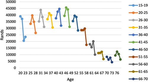
The cohort structure of our sample is summarised in Table 7. The total household income path based on cohort analysis shows a hump-shaped pattern where lower incomes are experienced during the post-retirement and younger working years (Figure 2). It can be seen that household income increases, peaking between ages 41 and 45. The cohort-wise analysis is limited by the potential differences between the two true household samples. While the first panel, 2002–04, shows an increase in household income, this trend is not continued in 2008. This fall could be because of lower mean income of the second true panel, 2008–10. Nevertheless the decline in the income levels of cohorts in 2008–10 is indicative of the macro shocks of the global financial crisis (Stats SA, 2013).

Figure 2: Household income

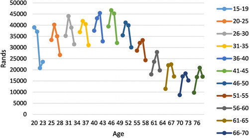
The trend is similar when tracing the path of total household income including incomes received from social grants such as old age pensions and the child support grant (Figure 3). However, cohorts aged 55 years and upward have higher total income as compared with household incomes of the same cohorts in Figure 2. This difference may be due not only to the old age pensions but also the child support grants received by the elderly to care for their grandchildren necessitated by the generation lost to HIV/AIDS in South Africa (Nyasani et al., 2009). Transfer payments from the government are thus observed to smooth the hump-shape by increasing the income levels in the post-retirement years.

Figure 3: Total household income (includes social grant receipts)

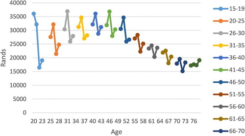
Figure 4 shows household consumption following a hump-shape. Household consumption across the cohorts is observed to increase, peaking between the ages of 31 and 35 before slowly declining. Unlike the expectations of smoothed consumption under the LCH, the consumption path is observed to potentially track income in South African households. Consumption levels estimated from the second panel are observed to be lower than the first panel. This indicates that although Table 5 showed the two panels to be comparable in terms of demographics, there seems to be a downward bias in consumption data of the second sample. Nevertheless, consumption is seen to be increasing over both panels, contrary to the trends observed in Figure 2 showing a decline in income in the years 2008–10. This indicates that households consider the decline in income to be transitory and hence continue to increase consumption by either incurring debt or dissaving (NCR, 2014).

Figure 4: Mean household consumption

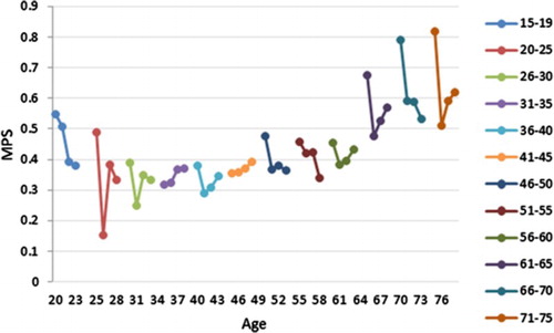
At first look, the marginal propensity to save of South African households, estimated using Equation (1), do not display the hump-shape expected from the LCH (Figure 5). However, the marginal propensity to save of the youngest cohorts up until the age of 31 is seen to be decreasing over the years. This can be attributed to the aspirational expenditures undertaken by the young. The marginal propensity to save of the middle-aged cohorts ranging from the age of 34 to 60 is seen to be stable between 30 and 40%. The marginal propensity to save of the oldest cohorts is seen to be the highest. This is against LCH expectations but in line with Deaton & Paxson (1994) and Poterba (1994), who attribute it to the bequest motive. In addition, it needs to be kept in mind that, given the low life expectancy in South Africa, the cohorts above 64 years old are likely to be those with higher income which enables them to save more. Sample bias could thus be the reason for household savings behaviour of the oldest cohorts.

Figure 5: Marginal propensity to save Note: MPS = marginal propensity to save.

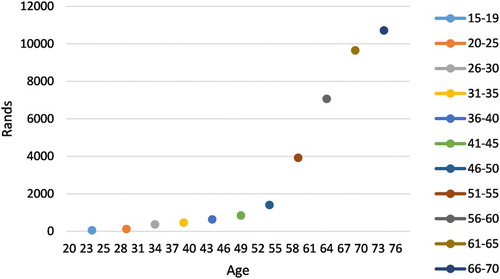
Figure 6 shows that social grant receipts are highest among the older cohorts. This is not surprising as old age pension in 2014 stood at R1350 per month whereas other grants such as child support was much lower at R320 per month (Government of South Africa, 2014). Following the trends in Figures 3 to 6, it appears as though the old age grants are utilised more for savings than for consumption. This is in keeping with evidence from Khayelitsha/Mitchell's Plain pointing to saving by the elderly to cover funeral expenses (Esson, 2003). Freire (2004c) also finds that savings in order to cover funeral costs in poorer South African society deter private wealth accumulation and inter-generational transfer of wealth. This argument runs counter to the bequest motive and highlights the importance of cultural factors in determining savings behaviour.

Figure 6: Mean household grants

6. Multivariariate regression results

While the graphical analysis in Section 5 provides interesting insights, the analysis does not allow us to conclude on the statistical significance of the differences between cohorts. Multivariate analysis undertaken in this section based on Equations (2) and (3) is expected to make up for this limitation.

Results of the pooled OLS, panel and 2SLS regression estimation of Equations (2) and (3) are presented in Tables 8 and 9 respectively. Both the Wu–Hausman F-statistic test and the Durbin–Wu–Hausman chi-squared test for endogeneity rejected the null of no endogeneity; hence we use the 2SLS results for interpretation where the wealth variable is instrumented with past wealth (Table 10).

Table 8: Consumption level (ln C) regression results

	Panel 1		Panel 2		Pooled OLS	2SLS
Variable	Fixed effects (1)	Random effects (2)	Fixed effects (3)	Random effects (4)	(5)	(6)
Log of income	0.269*** (0.018)	0.485*** (0.008)	0.232*** (0.021)	0.452*** (0.009)	0.477*** (0.006)	0.469*** (0.013)
Log of grant	0.011* (0.006)	0.006* (0.003)	0.008 (0.010)	0.012*** (0.003)	0.010*** (0.002)	0.016*** (0.004)
Age	0.070* (0.037)	0.014 (0.016)	−0.012 (0.053)	−0.026* (0.015)	0.003 (0.008)	−0.017 (0.016)
Age squared	−0.0006* (0.0003)	−0.00008 (0.0001)	−0.0003 (0.0004)	0.0003* (0.0001)	−0.00001 (0.00006)	0.0002 (0.0001)
Wealth	0.135*** (0.042)	0.364*** (0.019)	0.091 (0.084)	0.358*** (0.021)	0.363*** (0.014)	0.970*** (0.081)
Gender	–	0.098*** (0.023)	–	0.104*** (0.023)	0.108*** (0.016)	0.139*** (0.028)
Black	–	−0.395*** (0.019)	–	−0.360** (0.022)	−0.374*** (0.014)	−0.355*** (0.023)
Tertiary	0.128** (0.049)	0.405*** (0.023)	0.100 (0.049)	0.317*** (0.027)	0.369*** (0.017)	0.270*** (0.031)
Single	−0.037 (0.048)	−0.131*** (0.022)	−0.023 (0.050)	−0.168*** (0.022)	−0.151*** (0.015)	−0.182*** (0.027)
Urban	–	0.184*** (0.017)	–	0.120*** (0.019)	0.148*** (0.012)	0.140*** (0.020)
Household size	0.034*** (0.009)	0.015*** (0.003)	−0.010 (0.010)	0.022*** (0.003)	0.018*** (0.002)	0.014*** (0.004)
Cohort1	–	0.161 (0.222)	–	−0.190* (0.108)	−0.063 (0.067)	−0.157 (0.180)
Cohort2	–	−0.054 (0.121)	–	−0.057 (0.073)	−0.031 (0.044)	−0.0081 (0.131)
Cohort3	–	0.041 (0.075)	–	−0.005 (0.051)	0.005 (0.031)	−0.005 (0.077)
Cohort4	–	0.047 (0.043)	–	−0.043 (0.035)	−0.012 (0.022)	−0.064 (0.050)
Cohort6	–	−0.008 (0.034)	–	−0.026 (0.035)	−0.0008 (0.020)	−0.026 (0.044)
Cohort7	–	−0.083* (0.048)	–	−0.077 (0.053)	−0.036 (0.025)	−0.107 (0.069)
Cohort8	–	−0.065 (0.059)	–	−0.141* (0.080)	−0.026 (0.031)	−0.125 (0.097)
Cohort9	–	−0.114* (0.068)	–	−0.221* (0.115)	−0.054 (0.040)	−0.211 (0.136)
Cohort10	–	−0.088 (0.074)	–	−0.290* (0.157)	−0.030 (0.050)	−0.295* (0.159)
Cohort11	–	−0.035 (0.085)	–	−0.470** (0.212)	−0.022 (0.065)	−0.365* (0.199)
Cohort12	–	−0.082 (0.098)	–	−0.527* (0.271)	−0.039 (0.082)	−0.325 (0.236)
GFC dummy					−0.054** (0.021)	−0.014 (0.041)
Interest	−0.038*** (0.010)	−0.035*** (0.003)	−0.026*** (0.009)	−0.028*** (0.003)	−0.037*** (0.003)	(omitted)
Constant	5.583*** (1.344)	4.883*** (0.462)	9.319*** (1.790)	6.089*** (0.377)	5.328 *** (0.188)	5.354*** (0.460)
Observations	9 776	9 776	10 144	10 144	19 920	9318
R squared	0.45	0.60	0.06	0.42	0.51	0.36
Hausman test chi squared	245.82 (Prob>chi squared: 0.00)		196.89 (Prob>chi squared: 0.00)

Notes: Significant at ***1%, **5% or *10% level. The robust standard errors of all variables are presented in parentheses. #Model (6) 2SLS: Wealth variable is instrumented with lagged wealth variable.

Table 9: Ratio of consumption (ln(C/Y)) regression results

	Panel 1		Panel 2		Pooled OLS	2SLS
Variable	Fixed effects (1)	Random effects (2)	Fixed effects (3)	Random effects (4)	(5)	(6)
Log of income	−0.699*** (0.018)	−0.479*** (0.008)	−0.729*** (0.021)	−0.458*** (0.009)	−0.474*** (0.006)	−0.467*** (0.012)
Log of grant	−0.040*** (0.006)	−0.052*** (0.003)	−0.047*** (0.010)	−0.054*** (0.003)	−0.054*** (0.002)	−0.051*** (0.004)
Age	0.099*** (0.037)	0.024 (0.016)	0.008 (0.053)	−0.022 (0.015)	−0.0002 (0.006)	−0.019 (0.015)
Age squared	−0.0008 (0.0003)	−0.0001 (0.0001)	−0.0006 (0.0004)	0.0002 (0.0001)	0.00001 (0.00007)	0.0002* (0.0001)
Wealth	0.140*** (0.042)	0.356*** (0.019)	0.082 (0.085)	0.329*** (0.021)	0.345*** (0.014)	0.893*** (0.079)
Gender	–	0.115*** (0.023)	–	0.127*** (0.023)	0.126*** (0.016)	0.157*** (0.027)
Black	–	−0.388*** (0.018)	–	−0.353*** (0.022)	−0.367*** (0.014)	−0.347*** (0.023)
Tertiary	0.123** (0.049)	0.375*** (0.022)	0.092* (0.049)	0.266*** (0.026)	0.327*** (0.017)	0.227*** (0.030)
Single	−0.032 (0.048)	−0.126*** (0.022)	−0.016 (0.050)	−0.160*** (0.022)	−0.143*** (0.015)	−0.169*** (0.026)
Urban	–	0.177*** (0.017)	–	0.121*** (0.019)	0.146*** (0.012)	0.135*** (0.020)
Household size	0.035*** (0.009)	0.016*** (0.003)	−0.009 (0.010)	0.024*** (0.003)	0.020*** (0.002)	0.017*** (0.004)
Cohort1	–	0.293 (0.220)	–	−0.184* (0.108)	−0.084 (0.067)	−0.163 (0.178)
Cohort2	–	0.037 (0.121)	–	−0.056 (0.073)	−0.043 (0.044)	−0.081 (0.129)
Cohort3	–	0.094 (0.075)	–	−0.009 (0.051)	−0.004 (0.031)	−0.005 (0.075)
Cohort4	–	0.071* (0.042)	–	−0.046 (0.035)	−0.017 (0.022)	−0.065 (0.049)
Cohort6	–	−0.029 (0.034)	–	−0.022 (0.035)	0.00005 (0.020)	−0.024 (0.043)
Cohort7	–	−0.120** (0.048)	–	−0.058 (0.053)	−0.030 (0.0256)	−0.099 (0.067)
cohort8	–	−0.112* (0.058)	–	−0.112 (0.080)	−0.019 (0.031)	−0.111 (0.092)
Cohort9	–	−0.174** (0.067)	–	−0.141 (0.115)	−0.036 (0.040)	−0.181 (0.129)
Cohort10	–	−0.150** (0.074)	–	−0.175 (0.156)	−0.004 (0.050)	−0.257* (0.150)
Cohort11	–	−0.092 (0.084)	–	−0.329 (0.211)	0.011 (0.065)	−0.319* (0.186)
Cohort12	–	−0.110 (0.098)	2–	−0.363 (0.270)	0.013 (0.081)	−0.308 (0.221)
GFC dummy					−0.041* (0.021)	−0.005 (0.040)
Interest	−0.034*** (0.010)	−0.029*** (0.003)	−0.026*** (0.010)	−0.028*** (0.003)	−0.034*** (0.003)	(omitted)
Constant	4.514*** (1.347)	4.144*** (0.459)	8.447*** (1.800)	5.407*** (0.376)	4.882*** (0.188)	4.736*** (0.457)
Observations	9 776	9 776	10 144	10 144	19 920	9318
R squared	0.06	0.27	0.15	0.23	0.25	0.07
Hausman test chi squared	246.98 (Prob>chi squared: 0.00)		214.89 (Prob>chi squared: 0.00)

Notes: Significant at ***1%, **5% or *10% level. The robust standard errors of all variables are presented in parentheses. #Model (6) 2SLS: Wealth variable is instrumental with lagged wealth variable.

Table 10: Test of endogeneity of wealth dummy variable

	Consumption: 2SLS model	Ratio of consumption: 2SLS model
Wu–Hausman F-statistic test	129.549 (0.000)	109.593 (0.000)
Durbin–Wu–Hausman chi-squared test	125.16 (0.000)	106.151 (0.000)

The 2SLS estimation results lend some support to the LCH based on the positive and significant coefficients of household income, wealth and grants variables, combined with the insignificant age variables (Table 8). Although the coefficient of grant is significant, it is seen to be substantially lower than the coefficient of income in all estimations. This lends further support to the findings of Section 5 that older households, which are the major recipients of the grants, are saving a large proportion of it. This is in keeping with the evidence put forth by other studies such as Esson (2003) and Freire (2004c), who highlight the savings for funeral expenses in old age as a major deterrent of wealth creation and inter-generational transfer in South Africa.

The wealth coefficient is relatively high in all estimations and increases further in the 2SLS. The coefficients of income and wealth, however, cannot be directly compared because the former is a dummy variable. The coefficient of wealth can only be interpreted as the extent to which the wealthier households consume more than their poorer counterparts. It is therefore not surprising that the coefficient of wealth is larger than normally observed in other studies that look at the consumption smoothing effect of wealth. Although panel data estimations indicate some evidence of the age effect on consumption, this is only at a 10% significance level. They are able to do so not necessarily solely due to savings but because of the grants received from the government. The hump-shaped consumption revealed in the cohort analysis (Figure 4) is not revealed to be statistically significant in the regression results. The lack of strong cohort effects can be attributed to the low growth in real per-capita income levels in South Africa since the 1960s (Fedderke, 2014).

It is not surprising to see household size contributing positively to consumption. Urban, female-headed households with education are seen to have higher consumption levels compared with male-headed households without tertiary education. Being single and black, on the contrary, contributed to lower consumption levels.

Interest rates are seen to affect consumption negatively in all of the models, indicating that households respond when the inter-temporal benefits to save increases by saving more. It may also mean that for those spending on credit, consumption falls with an increase in the cost of borrowing. However, the variable could not be retained in the 2SLS estimation along with the GFC variable because of collinearity issues. The coefficient of the GFC dummy highlights the negative impact of the financial crisis on South African household consumption; however, this was not found to be significant in the 2SLS estimation.

Table 9 provides additional insights into consumption and saving behaviour of South African households by highlighting the determinants of the consumption–income ratio. An increase in income is, as expected, likely to reduce the consumption–income ratio, implying an increase in the rate of savings. Transfer income from the government is seen to have a similar but smaller impact on the consumption–income ratio. Ownership of wealth, however, is seen to increase the consumption–income ratio, implying wealth ownership reduces the motive to save further.

The insignificant coefficients of age and age-squared indicate that the consumption–income ratio, equally meaning the savings–income ratio, does not change over the life-span of the household head and goes against the LCH. This therefore contradicts our initial conclusions based on Table 8. Hence our argument that households are able to smooth their consumption not through savings but through government grants is strengthened. Households headed by educated, females and located in urban areas are seen to save less of their income as compared with male-headed household with no tertiary education located in rural areas. Results indicate that larger households are only able to save less of their income. An increase in the interest rate is observed to significantly reduce the consumption–income ratio in all of the models, indicating that households respond to higher returns on savings or the higher cost of borrowing. This variable, however, could not be included in the 2SLS estimation along with the GFC variable for the reasons aleady explained. The consumption–income ratio is observed to have decreased during the economic slowdown, indicating the precautionary motive to save in times of uncertainty. This is consistent with the reduced levels of consumption observed during this period from Table 8.

7. Conclusions

This cohort analysis shows that South African households achieve their income peaks in the early forties, while incomes in developed countries are seen to peak towards the late forties and fifties (Attanasio & Browning, 1994; Modigliani, 2005b). The reasons for this could potentially be attributed to the lower life expectancy of households in South Africa owing to the impact of HIV/AIDS (Freire, 2004a, 2004b). Although the cohort analysis reveals the hump-shape in income of households, the inclusion of transfer income is seen to smooth income levels, thus distorting the LCH premise of no income during retirement. The cohort analysis of the marginal propensity to save showed little variability across cohorts, although it was marginally higher, against expectations, in the oldest three cohorts. This may be accounted for by the bias generated by the higher probability of the rich to live longer and the saving of government grants by older households to finance funeral expenditures. The hump-shape of consumption revealed by the cohort analysis is not validated by our regression results.

Household savings in South Africa showed superficial support for the LCH framework through the evidence of smoothed consumption from our regression analysis. However, closer examination reveals that the consumption–income ratio is also smooth over the age and cohort variables. This indicates that savings rate do not change as required in the LCH framework over the life-span of an individual. The households are seen to be able to maintain their consumption in the retirement years through government grants. A large part of grants, however, is also seen to be channelled towards savings by the older households. Evidence from other micro studies in South Africa indicate that this savings by older households does not, however, lead to wealth creation or inter-generational transfer because it is maintained for funeral expenses. This shows that the government grants have the dual effect of sustaining consumption levels while disincentivising savings during the working years. This has fiscal and growth implications for the South African economy in the long term. The findings highlight the importance of taking into account cultural factors in understanding savings behaviour in South Africa.

This study is limited by the short panels used in the analysis. Further, the lack of quantitative wealth and savings data did not permit more rigorous testing of the LCH. However, the representative dataset and consistent results over the estimation models make our conclusions a benchmark for further micro-level research in South Africa.

Acknowledgments

The authors would like to thank the anonymous referees for their valuable comments. Any remaining errors are our own.

Disclosure statement

No potential conflict of interest was reported by the authors.

References

- Aron, J & Muelbauer, J, 2000. Personal and corporate saving in South Africa. World Bank Economic Review 14(3), 509–544. doi: 10.1093/wber/14.3.509
- Aron, J & Muelbauer, J, 2006. Estimates of household sector wealth in South Africa 1970–2003. Review of Income and Wealth 52(2), 285–307. doi: 10.1111/j.1475-4991.2006.00188.x
- Aron, J, Muelbauer, J & Prinsloo, J, 2007. Balance sheet estimates for South Africa's household sector from 1975 to 2005. Working Paper 01/07, SARB (South African Reserve Bank), Pretoria.
- Attansio, O & Browning, M, 1994. Testing the life cycle model of consumption: what can we learn from microeconomic and macroeconomic data? Investigaciones Economicas 18(3), 433–463.
- Belke, A, Dreger, C & Ochmann, R, 2012. Do Wealthier Households Save More: The Impact of the Demographic Factor. Discussion PaperNo. 6567, IZA Discussion Paper Series, May, Bonn.
- van der Berg, S, Sieberts, K & Lekezwa, B, 2010. Efficiency and Equity Effects of Social Grants in South Africa. Working Paper 15/10, Department of Economics, Stellenbosch University.
- Betrand, M, Mullainathan, S & Miller, D, 2003. Public policy and extended families: Evidence from pensions in South Africa. The World Bank Economic Review 17(1), 27–50. doi: 10.1093/wber/lhg014
- Browning, M & Crossley, T, 2001. The life-cycle model of consumption and savings. American Economic Association 15(3), 3–22.
- Browning, M & Lusardi, A, 1996. Household savings: Micro theories and micro facts. Journal of Economic Literature 34(4), 1797–1855.
- Carroll, CD & Summers, LH, 1991. Consumption growth parallels income growth: Some new evidence. In Bernheim, BD & Shoven, JB (Eds.), National saving and economic performance for the national bureau of economic research. Chicago University Press, Chicago, 305–348.
- Case, D & Deaton, A, 1998. Large cash transfers to the elderly in South Africa. The Economic Journal 108(450), 1330–1361. doi: 10.1111/1468-0297.00345
- Chauke, H, 2011. The determinants of household savings: The South African black middle class perspective. MBA dissertation, University of Pretoria.
- Chowa, G, 2006. Savings perfomarnce among rural households in Sub-Saharan Africa: The effect of gender. Social Development Issues 28(2), 106–116.
- Deaton, A, 1985. Panel data from time series of cross sections. Journal of Econometrics 30(1), 109–126. doi: 10.1016/0304-4076(85)90134-4
- Deaton, A. 1992. Understanding consumption. Oxford University Press, Oxford.
- Deaton, A & Paxson, C, 1994. Saving, growth, and aging in Taiwan. In Wise, DA (Ed.), Studies in the economics of aging. University of Chicago Press, Chicago, 331–362.
- Duflo, E, 2003. Grandmothers and granddaughters: Old age pensions and intrahousehold allocation in South Africa. World Bank Econ Rev 17(1), 1–25. doi: 10.1093/wber/lhg013
- du Plessis, G, 2008. An exploration of the determinants of South Africa's personal savings rate – Why do South Afircan Households Save so Little? Masters of Business Administration dissertation, University of Pretoria.
- Esson, R, 2003. Savings and savers: An analysis of saving behaviour among Cape Town's poor. Working Paper 59, CSSR(Centre for Social Science Research), University of Cape Town.
- Fedderke, J, 2014. Exploring unbalanced growth in South Africa: Understanding the sectoral structure of the South African economy. Working Paper 14/07, SARB (South African Reserve Bank), Pretoria.
- Freire, S, 2004a. Funeral Costs, Saving Behaviour and HIV/AIDS. Cahiers de la Maison des Sciences Economiques, Université Panthéon-Sorbonne. http://EconPapers.repec.org/RePEc:mse:wpsorb:bla04092 Accessed 3 March 2011.
- Freire, S, 2004b. Impact of HIV/AIDS on Saving Behaviour in South Africa. Proceedings of the African Development and Poverty Reduction: The Macro-Micro Linkage dPru-tiPs Cornell Univeristy Forum, 13–15 October. Somerset West, Western Cape, South Africa.
- Freire, S. 2004c. HIV/AIDS, funeral costs and wellbeing: Theory and evidence from South Africa. First Draft edn, TEAM, Université Paris I Sorbonne, Paris, France.
- Friedman, M, 1957. The Permanent Income Hypothesis. In Friedman, M (Eds.), A theory of the consumption function. Princeton University Press, Princeton, 20–37.
- Government of South Africa. n.d., n.d.-last update, Old age pension [Homepage of Government of South Africa], [Online]. http://www.gov.za/services/social-benefits-retirement-and-old-age/old-age-pension Accessed 20 February 2015.
- Government of South Africa, 2014. 28 October 2014-last update, Child support grant [Homepage of Government of South Africa], [Online]. http://www.gov.za/services/child-care-social-benefits/child-support-grant Accessed 20 Feburary 2015.
- Huang, KXD & Caliendo, F, 2011. Rationalising multiple consumption-saving puzzles in a unified framework. Frontiers of Economics in China 6(3), 359–388. doi: 10.1007/s11459-011-0138-0
- Jappelli, T, 1999. The age-wealth profile and the life-cycle hypothesis: A cohort analysis with time series of cross-sections of italian households. Review of Income and Wealth 45(1), 57–75. doi: 10.1111/j.1475-4991.1999.tb00312.x
- Keynes, JM, 1936. The definition of income, saving and investment. In Keynes, JM (Eds.), The general theory of employment, interest, and money. Harcourt Brace, New York, pp. 96.
- Lusardi, A, 2007. Implications of behavioural economics for economic policy report: Household savings behaviour in the United States: The Role of Literacy, Information, and Financial Education Programs. Boston.
- Mahlo, N, 2012. Determinants of Household Savings in South Africa. Masters disseration, Univeristy of Johannesburg.
- Mba, CJ, 2007. Impact of HIV/AIDS mortality on South Africa's life expectancy and implications for the elderly population. African Journal of Health Sciences 14(3), 201–210.
- Modigliani, F, 1986. Life cycle, individual thrift and the wealth of nations. American Economic Review 76(3), 297–313.
- Modigliani, F, 2005a. Utility analysis and the consumption function: An interpretation of cross section data. In Modigliani, F (Eds.), The collected papers of Franco Modigliani. The MIT Press, Cambridge. 3–45.
- Modigliani, F, 2005b. The age saving profile and the life-cycle hypothesis. In Modigliani, F (Eds.), The collected papers of Franco Modigliani. The MIT Press, Cambridge, 141–172.
- National Treasury of South Africa, 2012a. Technical Paper D Incentivising non-retirement savings. http://www.treasury.gov.za/comm_media/press/2012/Incentivising%20non-retirement%20savings.pdf Accessed 2 January 2013.
- National Treasury of South Africa, 2012b. Technical Paper E Strengthening retirement savings. http://www.treasury.gov.za/publications/RetirementReform/20120314%20-%20Strengthening%20retirement%20savings.pdf Accessed 2 January 2013.
- NCR (National Credit Regulator), 2014. Credit Bureau Monitor. National Credit Regulator, Pretoria. http://ncr.org.za/publications/Credit_Monitor/CBM%20March%202014..pdf Accessed 20 October 2014.
- Nyasani, E, Sterberg, E, & Smith, H, 2009. Fostering children affected by AIDS in Richards Bay, South Africa: a qualitative study of grandparents’ experiences. African Journal of AIDS Research 8(2), 181–192. doi: 10.2989/AJAR.2009.8.2.6.858
- Pistaferri, L, 2009. The life cycle hypothesis: An assessment of some recent evidence. Rivista di Politica Economica 99(2), 35–65.
- Poterba, J, 1994. International comparisons of household savings. University of Chicago Press, Chicago. doi: 10.7208/chicago/9780226676289.001.0001
- Prinsloo, J, 2000. The saving behaviour of the South African economy. Occasional Paper 14, SARB (South African Reserve Bank), Pretoria.
- Reserve Bank of India, 2014. Annal Report. https://rbi.org.in/scripts/AnnualReportPublications.aspx?Id=1120 Accessed 24 April 2015.
- Sachs, J & Malaney, P, 2002. The Economic and Social Burden of Malaria. Insight, February.
- Simleit, C, Keeton, G & Botha, F, 2011. The determinants of household savings in South Africa. Journal of Studies in Economics and Econometrics 35(3), 1–20.
- South African Reserve Bank, 2015. https://www.resbank.co.za/Publications/QuarterlyBulletins/Pages/QBOnlinestatsquery.aspx Accessed 24 April 2015.
- Spio, K & Groenewald, J, 1996. Rural household savings and the life cycle hypothesis: The case of South Africa. South African Journal of Economics 64(4), 217–223. doi: 10.1111/j.1813-6982.1996.tb01343.x
- Stats SA (Statistics South Africa), 2002, 2004, 2008, 2010. General Household Survey Annual Full Datasets of 2002, 2004, 2008 and 2010. Stats SA, Pretoria.
- Stats SA (Statistics South Africa), 2013. National and provincial labour market trends. Statistics South Africa, Pretoria.
- Verick, S, 2010. Unravelling the impact of the global financial crisis on the South African Labour Market. Working Paper No. 48, ILO (International Labour Office), Geneva.
- Wan, Junmin, 2011. Bubbly Savings. Working Paper No. 2011–010 Center for Advanced Economic Study, Fukuoka University, Japan.