Quantifying shifts in primary factor demand in the South African economy

ABSTRACT

This article uses a dynamic computable general equilibrium model to explain the persistence in the high levels of unemployment in the South African economy in spite of modest to relatively strong output growth. We make use of a historical simulation for the period 2006–13 and find that the capital–labour ratio increased despite a relative increase in the rental price of capital. Classical economic theory suggests that changes in industry preferences toward capital and labour lead to adjusted capital–labour ratios. We quantify the changes in industry factor preferences during this period and highlight their impact in explaining observed labour market outcomes. Other changes in the economy over this period are also quantified.

KEYWORDS:

• Capital–labour ratio
• unemployment
• computable general equilibrium model
• GEMPACK

JEL CLASSIFICATION:

• C68

1. Introduction

South Africa's rather puzzling unemployment problem has been well documented in articles and reports such as Pollin et al. (2006), Banerjee et al. (2008), Rodrik (2008) and Klein (2012). However, quantifying some of the factors and trends underlying the country's labour market problem remains a challenge. Over the period 2006–13, the South African economy showed encouraging real growth yet the number of employed persons increased only marginally, leaving the rate of unemployment around 25%. Rates of unemployment in the country's large stock of youth and low-skilled workers are particularly severe. In an attempt to better understand and quantify the factors that may have been responsible for employment growth not catching up with output growth, we analyse the South African economy, in particular its factor markets, within a general equilibrium framework, over the given period. Specifically, we conduct our analysis using the University of Pretoria General Equilibrium Model (UPGEM) with the historical decomposition model closure developed by Dixon & Rimmer (2002). This approach allows us to measure any shift in primary factor demand preferences that may help explain the phenomenon of persistently high unemployment in South Africa.

In addition to providing new quantitative analysis of trends in the primary factor environment, two ancillary benefits emerge from this research. First, we quantify various other trends in the macro economy such as trade preferences and technical changes that are useful for future baseline projections in UPGEM; and second, we update the model's underlying supply-use database.

The article is structured as follows. Section 2 describes the UPGEM methodology. Section 3 describes the model closure for the historical analysis and summarises the observed movements between 2006 and 2013. Section 4 presents the simulation results and Section 5 concludes.

2. Methodology

UPGEM is a recursive-dynamic computable general equilibrium (CGE) model of the South African economy. In this application of UPGEM we selected 2006 for the model's base year, based on the supply-use tables published in StatsSA (2008). The theoretical specification of UPGEM is based on the MONASH model of Australia described in Dixon & Rimmer (2002). The model is implemented and solved using GEMPACK described in Harrison & Pearson (1996), with simulation results typically reported in percentage change format.

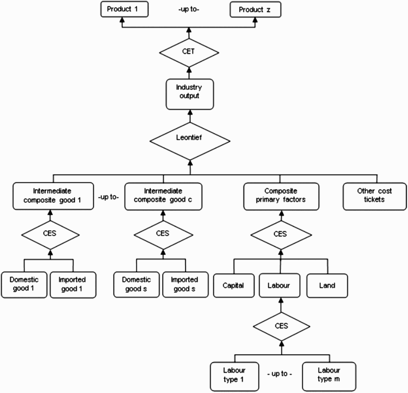
The specifications in UPGEM recognise each of the 33 industries in the model as producing one or more commodities, using as inputs combinations of domestic and imported commodities, different types of labour, capital and land. This multi-production specification is kept manageable by a series of separability assumptions, illustrated in Appendix A. The nested production structure reduces the number of estimated parameters required by the model. Optimising equations determining the commodity composition of industry output are derived subject to a constant elasticity of transformation function, while functions determining industry inputs are determined by a series of constant elasticity of substitution (CES) nests. At the top level of this nesting structure, intermediate commodity composites and a primary-factor composite are combined using a Leontief or fixed-proportions production function. Consequently, all inputs are demanded in direct proportion to industry output or activity. Each commodity composite is a CES function of a domestic good and its imported equivalent. This incorporates Armington's assumption of imperfect substitutability for goods by place of production (Armington, 1969). The primary-factor composite is a CES aggregate of composite labour, capital and, in the case of primary-sector industries, land. Composite labour demand is itself a CES aggregate of the different types of labour distinguished in the model's database. In UPGEM, all industries share this common production structure, but input proportions and behavioural parameters vary between industries based on base year data and available econometric estimates, respectively.

The demand and supply equations in UPGEM are derived from the solutions to the optimisation problems which are assumed to underlie the behaviour of private-sector agents in conventional neo-classical microeconomics. Each industry minimises cost subject to given input prices and a constant returns to scale production function. Zero pure profits are assumed for all industries. Households maximise a Klein–Rubin utility function subject to their budget constraint. Units of new industry-specific capital are constructed as cost-minimising combinations of domestic and imported commodities. The export demand for any locally produced commodity is inversely related to its foreign-currency price. Government consumption and the details of direct and indirect taxation are also recognised in the model.

The recursive-dynamic behaviour in UPGEM is specified through equations describing physical capital accumulation, lagged adjustment processes in the labour market and changes in the current account and net foreign liability positions. Capital accumulation is specified separately for each industry and linked to industry-specific net investment in the preceding period. Investment in each industry is positively related to its expected rate of return on capital, reflecting the price of capital rentals relative to the price of capital creation. For the government's fiscal accounts, a similar mechanism for financial asset/liability accumulation is specified. Changes in the public-sector debt are related to the public-sector debt incurred during a particular year and the interest payable on previous debt. Adjustments to the national net foreign liability position are related to the annual investment/savings imbalance, revaluations of assets and liabilities and remittance flows during the year. In policy simulations, the labour market follows a lagged adjustment path where wage rates respond over time to gaps between demand and supply for labour across each of the different occupation groups.

Despite the complex and large-scale structure of UPGEM, an intimate knowledge of CGE modelling is not necessary in order to understand the results from this article. In a typical general equilibrium model, we find a set of equations with naturally endogenous variables, including various prices and quantities, and naturally exogenous variables representing various preference or technical changes, the positions of demand or supply curves, and so forth. Since UPGEM contains many more variables (n) than equations (m), a number of variables (n – m) must therefore be set as exogenous in order to close the model and compute a solution. The essence of the historical closure used in this study is to exogenise many of these naturally endogenous, yet observable, variables and set an appropriate naturally exogenous variable in the corresponding equation as endogenous. For this reason, historical closures may at first appear unusual, in that many variables which we would consider to be naturally endogenous in policy modelling are now set exogenously at their historical values. A number of naturally exogenous variables must therefore be allowed to move endogenously for the model to maintain its compatibility with the given observed values and various parameter estimates over the historical period. By telling the model what happened to the components of gross domestic product (GDP), employment, wages, capital growth, rental prices, and so forth over the observed period of 2006–13, the historical closure allows the model to determine what happened to variables such as the average propensity to consume, technical change, capital/labour preferences, the positions of foreign export demand curves, and so forth over the same period. This helps us uncover trends within the model's detailed framework that may not have been possible otherwise.

As noted in Dixon & Rimmer (2013), historical simulations have become one of the main sources of statistical validation in CGE modelling and has been successfully used in studies such as Boratynski (2012), Dixon & Rimmer (2010), Giesecke & Tran (2009) and Mai (2007) to uncover interesting trends in unobservable variables. Readers interested in more of the technical details regarding the historical closure, or indeed the structure of large-scale CGE models, are encouraged to consult Dixon & Rimmer (2002:233–77) and Dixon et al. (2013).

3. Observed movements from 2006–13

As noted, we use a historical model closure to conduct our analysis of the South African economy for the period 2006–13. This requires us to provide the model with the relevant historical data for this period. Table 1 presents the variables in our model with explicitly assigned non-zero exogenous year-to-year movements based on available historical data. Pseudo-exogenous variables – that is, variables whose net change in any given period are determined by the exogenous variables – are shown in italics. Table 2 presents the same historical movements represented as cumulative percentage changes away from the 2006 base-year values or initial solution. With the components of GDP set at their observed values, real GDP growth of 20.2% was achieved over this period, equivalent to an average annual growth rate of around 2.6%.

Table 1. Annual percentage change to selected exogenous variables (2007–13).

	2007	2008	2009	2010	2011	2012	2013*
Macro variables
Real GDP (x0gdpexp)	5.5	3.6	−1.5	3.1	3.6	2.5	2.0
Real Consumption (x3tot)	5.5	2.2	−1.6	4.4	4.8	3.5	2.4
Real Investment (x2tot_i)	14.0	14.1	−3.2	−2.0	4.5	5.7	4.1
Real Government (x5tot)	3.9	4.5	4.6	5.0	4.6	4.2	3.3
Real Imports (x0cif_c)	9.0	1.5	−17.4	9.6	9.7	6.3	7.2
Real Exports (x4tot)	6.6	1.8	−19.5	4.5	5.9	0.1	6.0
Government/Consumption Ratio (f5tot)	−1.5	2.2	6.3	1.1	−0.5	0.5	1.0
Consumer Price Index (p3tot)	6.1	9.9	7.1	4.3	5.0	5.7	5.9
Real Wages (real_wage_c)	1.0	2.5	2.5	3.0	1.0	1.5	1.5
Terms of Trade (p0toft)	1.6	−0.1	8.0	7.2	2.3	−2.2	0.5
Nominal Exchange Rate (phi)	−4.6	−13.4	−2.3	14.0	1.3	−11.9	−10.0
Labour Employed (emp_jobs)	0.4	2.0	−3.0	−1.5	1.5	0.5	0.5
Capital Stock (x1cap)	1.7	2.9	4.0	3.5	3.0	3.1	3.4
Industry variables
Gold Price (p4)	31.0	4.0	25.0	30.5	7.5	8.5	−15.0
Gold Output (x4)	−5.5	−15.0	−6.0	−4.0	−4.0	−10.0	−5.0
Electricity Price (p0dom)	5.1	27.5	31.3	24.8	25.8	16.0	8.0
Electricity Output (z)	4.0	−1.0	−2.0	4.0	2.0	2.0	4.0

Note: Pseudo-exogenous variables – that is, variables whose net change in any given period are determined by the exogenous variables – are shown in italics.

Source: South African Reserve Bank (SARB), StatsSA, National Treasury, Eskom, *UPGEM simulation results.

Table 2. Cumulative percentage change to selected exogenous variables (2007–13).

	2007	2008	2009	2010	2011	2012	2013*
Macro variables
Real GDP (x0gdpexp)	5.5	9.3	7.6	11.0	15.0	17.9	20.2
Real Consumption (x3tot)	5.5	7.8	6.1	10.7	16.1	20.1	23.0
Real Investment (x2tot_i)	14.0	30.1	25.9	23.4	28.9	36.3	41.9
Real Government (x5tot)	3.9	8.6	13.5	19.2	24.7	30.0	34.2
Real Imports (x0cif_c)	9.0	10.6	−8.6	0.2	9.9	16.8	25.2
Real Exports (x4tot)	6.6	8.5	−12.6	−8.7	−3.3	−3.2	2.6
Government/Consumption Ratio (f5tot)	−1.5	0.7	7.0	7.6	7.5	8.1	9.2
Consumer Price Index (p3tot)	6.1	16.6	24.9	30.2	36.7	44.5	53.1
Real Wages (real_wage_c)	1.0	3.5	6.1	9.3	10.4	12.0	13.7
Terms of Trade (p0toft)	1.6	1.5	9.6	17.5	20.2	17.5	18.1
Nominal Exchange Rate (phi)	−4.6	−17.4	−19.3	−8.0	−6.8	−17.9	−26.1
Labour Employed (emp_jobs)	0.4	2.4	−0.6	−2.1	−0.7	−0.2	0.3
Capital Stock (x1cap)	1.7	4.7	8.9	12.7	16.0	19.5	23.4
Industry variables
Gold Price (p4)	31.0	36.2	70.3	122.2	138.9	159.2	120.3
Gold Output (x4)	−5.5	−19.6	−24.5	−27.5	−30.4	−37.4	−40.5
Electricity Price (p0dom)	5.1	34.0	75.9	119.6	176.2	220.4	246.0
Electricity Output (z)	4.0	2.9	0.9	4.9	7.0	9.1	13.5

Note: Pseudo-exogenous variables – that is, variables whose net change in any given period are determined by the exogenous variables – are shown in italics.

Source: SARB, StatsSA, National Treasury, Eskom, *UPGEM simulation results.

Apart from the main macro variables, Tables 1 and 2 also show industry variables in the gold and electricity sectors that were exogenously assigned their observed values. Both of these industries are of special importance to the local economy. Despite falling output levels, South Africa remains one of the leading gold producers in the world, yielding significant export revenues. The electricity sector in South Africa is heavily regulated through the state-owned enterprise Eskom. Since 2007 and the commencement of Eskom's New Build Programme, electricity prices have increased significantly in order to reach a cost-reflective level (Eskom, 2013). By combining available price and output data for these sectors, we are then able to endogenously estimate changes in productivity and shifts in demand curves required to reconcile these observations with relevant elasticity parameter values in the model.

Figures 1 and 2 display the same information as Table 2 for selected variables in line chart form. Figure 1 shows the cumulative percentage change in import versus export quantities and of persons employed versus capital stock. South Africa's widening trade deficit and the impact of the global financial crisis in 2008/09 on trade are clearly evident, as well as the poor performance of the labour market, in terms of employment numbers, relative to the growth in the capital stock. Figure 2 shows the cumulative movement in important price variables.

Figure 1. Cumulative percentage change to trade, capital and labour variables (2007–13)

Source: SARB, StatsSA.

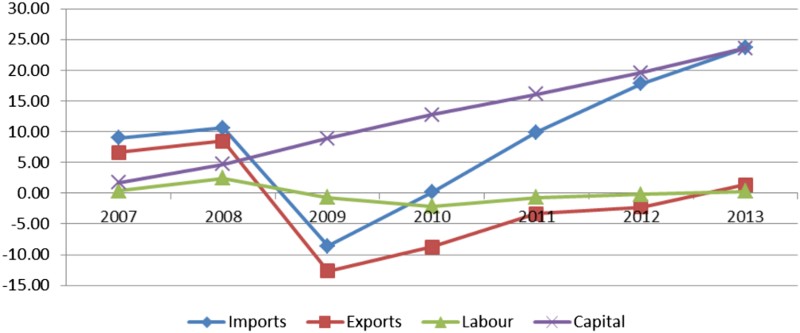
Figure 2. Cumulative percentage change to selected price variables (2007–13)

Source: SARB, StatsSA, UPGEM simulation results.

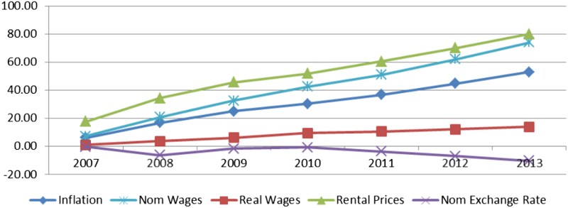
The most interesting observation that emerges from the data is the relative increase in the use of capital relative to labour (see Figure 1), despite increases in the relative price of capital rentals (endogenously determined here) to wages (see Figure 2). In the following section we discuss the solutions to various endogenous variables that help explain this apparent contradiction.

4. Endogenous results for the historical simulation: 2006–13

Given the choice of closure and ‘historical’ exogenous shocks to the model over the observed period, UPGEM determines the movement in a large number of endogenous variables. Tables 3–4 show the endogenous variables most relevant to our analysis of the selected macro and industry observations in Section 3, relative to movements in overall factor productivity, preference twists between domestic and imported commodities used by industry, shifts in the rest of the world's demand for our exports and preference twists between capital and labour reflecting changes in industry technology. We also show productivity change in the gold industry. Results in Table 3 are shown as annual percentage changes and in Table 4 as cumulative percentage changes.

Table 3. Annual percentage change to selected endogenous variables (2007–13).

	2007	2008	2009	2010	2011	2012	2013*
Endogenous macro variables
Factor productivity (ff_a1prim)*	5.0	3.3	−2.0	1.3	2.1	1.4	0.8
Import/domestic pref (twist_c)	2.5	−8.1	−31.1	5.8	4.9	8.0	2.0
Export demand shift (f4gen)	6.1	−1.8	−7.5	20.7	10.2	−5.9	5.3
Labour/capital preference (twist_i)	3.2	1.0	11.2	5.6	0.8	2.3	2.9
Endogenous industry variables
Gold export demand shift (f4q)	20.6	−25.4	41.4	31.5	−5.3	−8.9	−34.5
Gold factor productivity (f_a1prim)*	16.7	18.9	4.3	10.3	10.8	13.8	−1.1

Source: *UPGEM simulation results.

Table 4. Cumulative percentage change to selected endogenous variables (2007–13).

	2007	2008	2009	2010	2011	2012	2013*
Endogenous macro variables
Factor productivity (ff_a1prim)*	5.0	8.3	6.4	7.6	9.6	10.9	11.6
Import/domestic pref (twist_c)	2.5	−5.8	−35.1	−31.3	−27.9	−22.2	−20.7
Export demand shift (f4gen)	6.1	4.2	−3.6	16.3	28.1	20.5	26.9
Labour/capital preference (twist_i)	3.2	4.2	15.9	22.4	23.4	26.4	30.0
Endogenous industry variables
Gold export demand shift (f4q)	20.6	−10.8	27.1	67.3	58.4	44.2	−5.5
Gold factor productivity (f_a1prim)*	−16.7	−38.7	−44.7	−59.6	−76.9	−101.2	−99.0

Source: *UPGEM simulation results.

The most striking result from our historical simulation relates to the changes in primary factor composites – that is, the combination of capital and labour – by industry. The historical data in Section 3 show an increase in the observed capital–labour (K/L) ratio over the period 2006–13 despite an increase in the rental–wage ratio (P_K/P_L). Holding ‘all other things equal’, this result seems to defy conventional theory. To explain how the economy changed during this period to make this result possible, we introduce the concept of a cost-neutral preference twist from Dixon & Rimmer (2002, 2004).

4.1 Explaining the observed capital–labour changes

To calibrate the increase in the K/L ratio with the historical increase in the cost of using capital relative to labour, a cost-neutral labour/capital preference twist, shown below as TWLK, is introduced. Intuitively, the TWLK twist variable may be thought of as a variable capturing changes not explained by conventional substitution between capital and labour as a result of relative price changes.

Over the period 2006–13 the model generates a cost-neutral twist in preferences by users of labour in the primary-factor composite. The positive value of 30.0% generated for TWLK (twist_i) over the period, as shown in Table 4, reflects a strong shift in preferences away from the use of labour required by the model to reconcile the seemingly incompatible exogenously given values of the K/L ratio and primary-factor prices in Tables 1 and 2.

To explain this result we must look at the theoretical specification of TWLK within UPGEM. Input demand equations by industries are derived subject to a CES aggregation function with substitution elasticities (σ) between primary factors set at 0.2. Setting σ ≠ 1 in the linearised input demand equations allows cost-neutral preference twists (TWLK) accommodating exogenous historical data or forecasts in the primary-factor market to be introduced and converted into technical or taste changes.¹ Equations (1) and (2) show these linearised demand equations as they appear in the UPGEM model code:(1) (2)

Following the UPGEM notation, cap and lab represent the percentage change in industry demands for capital (K) and labour (L), respectively. We note that in the absence of any change in output (z) and relative factor prices (p_K – p_L), this representation gives [cap – lab = TWLK] and [S_K*cap + S_L*lab = 0]. Thus, if the K/L ratio in UPGEM increases by 10% beyond what is explained by relative factor price movements, then TWLK will equal 10. The twist is therefore equivalent to movements in a_K and a_L – the technical change associated with capital and labour, respectively, which satisfy equations (3) and (4):(3) (4)

We can further show that by implementing the twist via the technical change variables, we are in effect assuming that and . With below one, a positive TWLK value is equivalent to a cost-neutral capital-using technical change combined with a labour-saving technical change.

To provide additional insight into the composition of our K/L movements, we use the two ‘back-of-the-envelope’ formulae shown in equations (5) and (6).² Assuming competitive conditions, the marginal products of capital and labour would equal their respective factor payments. In our exposition of equation (5) we recognise that the marginal product of capital (F_K) is negatively related to the K/L ratio. In equation (6) we recognise that the marginal product of labour (F_L) is positively related to the K/L ratio. In determining equation (5) we assume that the rate of return on capital can be expressed as (Q/P_i), with Q the factor payment to capital and P_i the price index for new investments. We then assume that Q is determined by the value of the marginal product of capital, written as (F_K*P_y). With (F_K) a function of the K/L ratio, and technical change (A) and (P_y/P_i) a function of the terms of trade (TofT), we are able to summarise this relationship through equation (5). In similar fashion, we are able to write equation (6) linking the real wage (W/P_c) to the K/L ratio, technical change and the terms of trade effect:(5) (6)

Given the implementation of our labour/capital twist via the technical change variables, we are now able to use our ‘back-of-the-envelope’ equations to help interpret the results for TWLK. In equation (5), a preference twist affecting capital will therefore be transmitted via the technical change variable (A_K). In equation (6), a preference twist affecting labour will similarly be transmitted via the technical change variable (A_L).

Our simulation results show strong primary-factor technical change in favour of capital and against labour between 2007 and 2013. This is reflected in the positive value of 30.0% generated for TWLK (twist_i). We may equate this result to an increase in A_K in equation (5) which will decrease the marginal product of capital requiring a rise in the relative amount of capital used. For labour, this may be equated to a decrease in A_L in equation (6), which will increase the marginal product of labour requiring a fall in the relative amount of labour used.

This result suggests that industry technology on average changed to the extent that for any given ratio of the real wage to the real rental price of capital, industries would choose a K/L ratio 30% higher in 2013 than in 2006. This change may also be interpreted as a change in ‘preferences’ by industry for their primary-factor composite. More capital is now preferred relative to labour in the production process, all other things equal.

To find the exact reasons for the change in industry technology or preferences towards the use of capital requires further research. However, it is no secret that rigid labour market conditions and labour unrest do have an impact on South African firms’ attitudes to hiring labour. The result also shows to what extent capital–labour substitution is possible.

With employment (emp_jobs) exogenous and capital growth (x1cap) linked to investment expenditure (x2tot) via the capital accumulation mechanism, the model shows that an economy-wide technical change (ff_a1prim) of 11.6% occurred over this period. That is, the model calculates that a cumulative productivity increase of 11.6% was required to calibrate the observed GDP figures with changes in use of capital and labour inputs. This is in line with international estimates that calculate productivity growth to be the largest contributor to economic growth.

Given the exogenous export demand (x4tot) and terms of trade (p0toft), a cumulative shift in the world demand for exports (f4gen) of 26.9% is endogenously determined by the model. The shift in export demand reflects the general growth in the world economy and demand for locally-produced exports, consistent with the exogenous trade data. This result is equivalent to an annual average growth rate, or outward shift, of around 3.5% in the export demand curve (f4gen) over the seven-year period. To explain this result, recall from Section 2 that the export–demand curve is downward sloping. A large shift in (f4gen) is therefore required for the model to reconcile the exogenously given increase in real exports (x4tot) of 2.6% with the increase in the terms of trade (p0toft) of 18.1%. The result reflects the assumed export demand elasticities in UPGEM of between 1.5 and 3 for all commodities.

The lower levels of trade relative to GDP (x0gdpexp) in the period 2008–09 reflect the impact of the Global Financial Crisis on imports (x0cif_c) and exports (x4tot). The terms of trade (p0toft) is shown to have improved between 2007 and 2013. This is defined as an increase in export prices relative to import prices. A natural shift towards relatively cheaper imports in the local import/domestic sales mix should therefore occur. However, the observed values for imports and exports do not suggest any significant change in the import/domestic mix relative to the given change in the terms of trade. To calibrate the historical values for the trade balance with the terms of trade, a cost neutral import/domestic preference twist (twist_c) is introduced in a similar fashion to the capital/labour twist. Over the period 2006–13, a cost-neutral twist in preferences by users to substitute imports of intermediates with local inputs in the local/import domestic mix of sales is generated by the model. The negative value of 20.7% generated for the import/domestic preference twist (twist_c), as shown in Table 4, reflects this shift in preferences away from the use of imports required by the model to reconcile the different exogenously given values of imports, exports and terms of trade in Tables 1 and 2. One plausible reason for this shift may be attributed to changes in government procurement policies favouring locally produced goods.

5. Conclusions

South Africa's GDP growth and unemployment problems are well documented in the literature. This article seeks to quantify some of the factors underlying the economy's weak labour absorption rate and employment growth that is far weaker than output growth. The results from the historical CGE simulation show that there has been a significant shift in preferences away from labour towards capital and that industry technology on average changed so that, at any given ratio of the real wage to the real rental price of capital, industries would choose a K/L ratio 30% higher in 2013 than in 2006. Reasons for this shift in industry preferences away from labour, which helps explain South Africa's poor employment growth despite moderate real GDP growth, requires further research, but may point to the role of poor educational outcomes, skill shortages and the role of labour unions in costly, protracted industrial action protests.

Other findings include a slight improvement in overall primary-factor technical change, but a significant deterioration in productivity in the gold sector, perhaps as a result of the increasing difficulty associated with deep underground mining. A slight preference twist towards the use of domestically produced goods relative to imports was also found. The findings from this article lay the groundwork for improved baseline forecasts for the UPGEM model and a better understanding of recent trends in the economy.

Acknowledgement

The authors gratefully acknowledge Economic Research Southern Africa (ERSA) in respect of a grant for the original version of this paper published in the ERSA working paper series, Working Paper No. 416, under the title ‘A Historical CGE Simulation of the South African Economy from 2006–2013: Analysing the Changes in the Use of Primary Factors by Industries’.

Disclosure statement

No potential conflict of interest was reported by the authors.

Additional information

Funding

The authors received a grant from Economic Research Southern Africa.

Notes

¹This method of implementing cost-neutral preference twists eliminates a problem arising with these variables when set as exogenous in policy simulations. The same method is used to implement cost-neutral import/domestic preference twists.

²The two ‘back-of-the-envelope' formulae in equations (5) and (6) are easily derived by maximising economy-wide profits, P_y.Y – (W.L + Q.K), subject to a Cobb–Douglas production function where Y = A[L^β.K^{(1 – β)}].

Appendix A. Nested production structure of a representative industry in UPGEM

References

- Armington, PS, 1969. A theory of demand for products distinguished by place of production. Staff Papers – International Monetary Fund 16, 159–178. doi: 10.2307/3866403
- Banerjee, A, Galiani, S, Levinsohn, J, McLaren, Z & Woolard, I, 2008. Why has unemployment risen in the new South Africa? Economics of Transition 16, 715–740. doi: 10.1111/j.1468-0351.2008.00340.x
- Boratynski, J, 2012. Historical Simulations with a Dynamic CGE Model: Results for an Emerging Economy. Paper prepared for the 2012 Ecomod Conference, Seville.
- Dixon, PB & Rimmer, MT, 2002. Dynamic general equilibrium modelling for forecasting and policy: A practical guide and documentation of MONASH. North-Holland, Amsterdam.
- Dixon, PB & Rimmer, MT, 2004. A problem with exogenous twists in policy. CoPS Archive Item TPPB0053. www.monash.edu.au/policy Accessed 30 June 2014.
- Dixon, PB & Rimmer, MT, 2010. Validating a detailed, dynamic CGE model of the USA. The Economic Record 86, 22–34 (Special Issue). doi: 10.1111/j.1475-4932.2010.00656.x
- Dixon, PB & Rimmer, MT, 2013. Validation in CGE modelling. In Dixon, PB & Jorgenson, DW (Eds.), Handbook of computable general equilibrium modelling. North-Holland, Amsterdam.
- Dixon, PB, Koopman, RB & Rimmer, MT, 2013. The MONASH style of CGE modelling. In Dixon, PB & Jorgenson, DW (Eds.), Handbook of computable general equilibrium modelling. North-Holland, Amsterdam.
- Eskom, 2013. Tariff & charges booklet 2013/14. www.eskom.co.za/tariffs Accessed 30 June 2014.
- Giesecke, J & Tran, NH, 2009. Sources of growth and structural change in the Vietnamese economic 1996–2003: A computable general equilibrium analysis. Asian Economic Journal 23(2), 195–224. doi: 10.1111/j.1467-8381.2009.02009.x
- Harrison, WJ & Pearson, KR, 1996. Computing Solutions for Large General Equilibrium Models using GEMPACK. Computational Economics 9, 83–127. doi: 10.1007/BF00123638
- Klein, N, 2012. Real wage, labour productivity and employment trends in South Africa: A closer look. IMF Working Paper 12/92. International Monetary Fund, Washington, DC.
- Mai, Y, 2007. The Chinese economy from 1997–2015: Developing a baseline for the MCHUGE model. CoPS/IMPACT Working Paper G-161. Centre of Policy Studies, Monash University, Melbourne.
- Pollin, R, Epstein, G, Heintz, J & Ndikumana, L, 2006. An employment-targeted economic program for South Africa. United Nations Development Programme, New York.
- Rodrik, D, 2008. Understanding South Africa's economic puzzles. Economics of Transition 16, 769–797. doi: 10.1111/j.1468-0351.2008.00343.x
- StatsSA (Statistics South Africa), 2008. Gross Domestic Product, Fourth Quarter 2007. Statistical Release P0441. Statistics South Africa, Pretoria.