The growth, poverty and inequality nexus in South Africa: Cointegration and causality analysis

ABSTRACT

This study empirically established the long-run relationship and causality effects that exist between growth, poverty and inequality. The analysis was carried out on a panel of nine South African provinces from 1995 to 2012. To capture poverty and inequality in a broader context, two measures of poverty (income and non-income) and three measures of inequality (income, education and land) were adopted for the study. The results confirm that there is a long-run relationship between growth, poverty and inequality. Notable results from the causality tests suggest that growth does not promote equal distribution of income in society but as income distribution begins to equalise, economic growth rises. This is regarded as growth–inequality disconnect. The unidirectional causality, which runs from income poverty to income inequality, suggests that a rising level of income poverty will lead to falling income inequality in the society; likewise, income inequality increases as non-income poverty declines.

Keywords:

• Growth
• poverty
• inequality
• cointegration
• causality
• South Africa

JEL CLASSIFICATIONS:

• I24
• I32
• O40
• O55
• C26
• C23

1. Introduction and background

Growth, poverty and inequality – also referred to as the triple challenges – continue to remain an important discourse in both the policy and the intellectual environments. Whether policies that promote growth will lead to a reduction in poverty and inequality (or whether a poverty-alleviated society translates into equal distribution or equal access to financial, natural and human resources within the society) remains a difficult question to answer. As South Africa remains one of the focal economies that continue to experience the triple challenges, this study aimed at investigating the existence of a long-run relationship and the direction of causality between the three variables.

In analysing the growth–poverty–inequality nexus, Bourguignon (2003) points out that the real challenge in establishing a development strategy lies not in the relationship that exists between poverty and growth on the one hand and poverty and inequality on the other, but in the interaction between inequality and growth. Bourguignon's assertion is based on the reasoning that there is almost consensus (Kakwani, 1993; Deininger & Squire, 1996; Dollar & Kraay, 2002) among economists that growth leads to poverty reduction and rising inequality increases poverty, but it is still difficult to ascertain whether growth causes inequality and/or inequality causes growth. Although, Heshmati (2004) found it difficult to measure the effects of inequality and growth on efforts to reduce poverty in developing countries, he suggests that economic growth could benefit the poor; however, if effective redistribution policies are absent, this might affect income distribution adversely. In this study, this issue was further investigated on the empirical front by augmenting the argument with non-income measures of poverty and inequality.

Recent literature predicting the relationship between growth and poverty reveals the non-existence of poverty convergence when poverty is measured at the absolute level, but when the severity of poverty – capturing the level of inequality – is taken into consideration, poverty convergence tends to exist (Kraay, 2006; Ghani et al., 2012; Ravallion, 2012). Empirical evidence on the relationship between growth and inequality reveals dual causality effects. On the one hand, there is evidence of a negative effect of inequality on growth (Alesina & Rodrik, 1994; Person & Tabellini, 1994) and, on the other, the effect of growth on inequality remains ambiguous (Roine et al., 2009). This can be ascribed to Kuznet's (1955) hypothesis, which suggests that at the initial low level of economic growth, income inequality is low, but as growth increases, inequality also increases – until a threshold is reached, after which inequality declines as growth rises. This means that the sign of the growth effect on inequality depends on the developmental stage in which an economy finds itself. Since growth affects both poverty and inequality in one way or another, the relationship between poverty and inequality is expected to be bidirectional. In other words, poverty and inequality affect each other through their link with economic growth (ODI, 2002).

Global efforts to eliminate absolute poverty are important, but it is also necessary to have country-specific combinations of growth and distribution policies. An increasing level of economic growth could lead to rising levels of inequality in the society if what is driving the former is not inclusive (Bourguignon, 2003). Empirical literature (Ravillion, 1997, 2001; Kanbur, 2005) suggests low inequality–growth elasticities. In other words, income inequality can only be reduced if there is a significantly high level of economic growth. Countries with high initial levels of income inequality could experience lower growth–poverty elasticity than countries with low initial levels of income inequality. However, very high levels of inequality could be bad for economic growth. To establish a better development strategy, various authors further decomposed changes in poverty into a growth component and a redistribution component (Datt & Ravallion, 1992; Ravallion & Chen, 1997; Adams Jr & Page, 2003; Adams Jr, 2004).

Over the past decade, the focus has been more on achieving higher and sustained economic growth in an effort to achieve the Millennium Development Goal of reducing poverty; however, at the same time, the equally important factor of how the generated income should be distributed within the economy has been neglected. While poverty has decreased across the regions in the past decades (due to rising income), inequality has increased, dampening the impact of growth on poverty reduction (Balarkrishnan et al., 2013). This trend indicates that the rising economic growth of the past decades has not been inclusive enough and therefore a more inclusive/pro-poor economic policy is needed to eradicate relative poverty in the world (Saad-Filho, 2010).

The existing South African literature (Leibbrandt et al., 2001, 2006; Bhorat & Van der Westhuizen, 2007; Bhorat et al., 2009; Van der Berg, 2010) has provided extensive empirical analysis on both income and non-income poverty and inequality levels and trends, but did not examine the causal relationship between poverty, inequality and growth.

The evolution of real gross domestic product (GDP; measure of growth), poverty and inequality in South Africa has revealed some basic trends over the past decade or two. Income poverty and income inequality have been used extensively in the literature as a measure of the overall level of poverty and inequality in society; whereas poverty of deprivation and social (land and education) inequality are an equally or more important measure of overall poverty and inequality. Evidence for these non-income poverty and inequality measures in society is more susceptible to trigger social violence and damage the existing social cohesions than income measures of poverty and inequality.

Figure 1(a) and (b) shows the different measures of poverty and inequality in South Africa.¹ In the midst of a rising level of real GDP, both income and non-income poverty have been on a falling trend, suggesting that South Africa might have partaken in meeting the Millennium Development Goal of halving poverty in the world (Figure 1(a)). In terms of provincial poverty levels, Gauteng and Western Cape recorded the worst income poverty index in the country and stand above the national income poverty level. On the other hand, these two provinces are the best-performing provinces in the country in relation to non-income poverty (Figure A1 in Appendix A).²

Figure 1. GDP, poverty and inequality performances in South Africa. Source: South African Reserve Bank, Statistic South Africa via Quantec EasyData database, World Bank Databank, African Development Indicators.

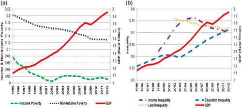
Looking at the trend in inequality, Figure 1(b) shows the performances of income, land and education inequality using the Gini index. Despite falling poverty levels, inequality remains relatively high in South Africa. In general, across all nine provinces of South Africa, the level of income inequality rose steadily and reached its peak (0.76) in 2005, and declined subtly to 2008 and thereafter remained relatively unchanged. Gauteng and Western Cape recorded the best income inequality index in the country as they stand below the national income inequality level (Figure A1 in Appendix A). With regard to the distribution of education outcomes per citizen and across all nine provinces in South Africa, the level of education inequality rose steadily, especially since 2003. In 2012 the Gini education index at the national level stood at about 0.71, confirming that the highest education attainment remained concentrated towards the few in the society (Figure 1(b)). This is paradoxical in that about 20% of the country's budget went to education and yet little outcomes have been recorded over the years. Except for Gauteng and the Western Cape, education inequality in the rest of the provinces was clustered around the same mean and was slightly above the national average (Figure A1 in Appendix A). Land distribution remains one of the most debatable socio-economic issues in South Africa. In 2012 the overall economy Gini (land) index was about 0.72, trending downward from 0.76 in 2002 (Figure 1(b)). The Eastern Cape, Kwazulu-Natal and Limpopo provinces contributed to this downward trend, and are regarded as the best-performing provinces in terms of the Gini (land) index (Figure A1 in Appendix A).

To support this debate on the growth–poverty–inequality nexus, it is important to establish the existence of a long-run relationship among these variables as well as the direction of causality between them. This exercise remains rare in the empirical literature. However, in a panel data setting from the nine provinces of South Africa, the long-run relationship and the causal effects that exist between growth, poverty and inequality was investigated. Preference for provincial panel data analysis was strictly because of data availability. What further distinguishes this study from related studies is the ability to augment the popular measure of income poverty and inequality with non-income poverty and inequality. The use of a panel data econometric technique was justified on the basis that there were limited data available to carry out robust time-series econometric specification. Therefore, the pooling of time and cross-sections improved the efficiency of the estimation parameters.

The results confirm that long-run relationships exist between growth, poverty and inequality, even when the different measures of poverty and inequality are adopted. In terms of the causality effect, there are unidirectional causal effects among the variables in most cases. There are bidirectional causality effects between growth and income poverty, growth and income inequality, and land inequality and non-income poverty. However, the results found no causality between land inequality and income poverty.

The rest of the study is organised as follows: Section 2 concerns the theoretical framework, methodology and estimation techniques that were adopted for the study, as well as the data analysis; Section 3 contains an analysis of the various estimation results; and Section 4 is the conclusion of the study, with the policy implications.

2. Theoretical framework, methodology and data analysis

2.1 Theoretical framework

The link between growth, poverty and inequality is established in the literature and can be represented in the form of a growth–poverty–inequality triangle.

In Bourguignon's (2003) growth–poverty–inequality triangle, changes in poverty are decomposed into the growth effect and the distribution (inequality) effect. This framework was adopted from the seminal papers of Datt & Ravillion (1992) and Kakwani (1993). In Figure 2, the growth effect of poverty implies a proportional change in aggregate income that leaves the distribution of relative income unchanged, while the distribution effect of poverty implies a change in the distribution of relative incomes that leaves aggregate income unchanged. This unidirectional relationship between growth, poverty and inequality was further investigated in this study by testing the existence of bidirectional causal relationships among these three variables. In other words, do poverty levels explain growth and inequality and/or what is the causal relationship between growth and inequality?

Figure 2. The poverty–growth–inequality triangle. Source: Bourguignon (2003).

2.2 Methodology

The methodology for the study was based on a recently developed panel cointegration test and a panel causality test from the combined Johansen–Fisher (Maddala & Wu, 1999) and Dumitrescu & Hurlin (2012) panel causality tests respectively. To carry out these investigations, it was important to understand the nature of the data-generating process. First, the order of integration (stationarity test) of the variables is tested. Second, if integration of order one (I[1]) is found in at least one variable, then it is necessary to proceed to test for cointegration among the variables, but if all the variables are integrated at order zero (I[0]), this means that they are cointegrated and have long-run relationships. The final step is to employ a dynamic panel causality test to detect the direction of causality among the variables.

The Levin et al. (2002), Im et al. (2003) and Fisher-type (proposed by Maddala & Wu, 1999) panel unit root tests were used in the study.

Given that one or more of the variables have unit roots, the combined Johansen (1988) and Fisher's (1932) panel cointegration test was adopted for the study. Maddala & Wu (1999) refer to Wu's (1998) thesis, which suggested that a Fisher-type panel cointegration test is more appropriate since it provides allowance for some relationships to be cointegrated and others not to be cointegrated. Therefore, the Johansen–Fisher panel cointegration test combines tests from individual cross-sections to obtain test statistics for a full panel.

Since two measures of poverty (income and non-income) and three measures of inequality (income, education and land)³ were used in this study, the cointegration tests between poverty, growth and inequality took the form of the following reduced-form vector autoregression (VAR):(1)

Equation (1) is in line with the Johansen (1988) cointegration estimation technique, as set out in Enders (2004:348) and where is a vector of variables:(2) (3) (4) (5) (6) (7)

where is the level of real GDP, is the income inequality, is the income poverty, is the non-income poverty, is the education inequality and is the land inequality. Adopting Cholesky decomposition for orthogonalisation, and where the Cholesky factor is found to be triangular, each variable in the vector is therefore allowed to react contemporaneously to all variables above it (Enders, 2004:270). This means that poverty will be influenced, contemporaneously, by all the other variables.

After detecting the existence of long-run relationships among the variables, the direction of causality between these variables was further investigated. The Dumitrescu & Hurlin (2012) panel causality test that was adopted in this study assumes that all coefficients are different across cross-sections and, therefore, the bivariate regressions are run for individual cross-sections and the average of the test statistics (herein referred to as W-statistics) are taken to represent the full panel. In a panel data context, the general bivariate regressions take the following form:(8) (9)

Based on the Dumitrescu-Hurlin approach, and .

However, given the different measures of poverty and inequality that were used in the study, 11 panel causality tests were performed. In addition, the direction of causality was buttressed by running an individual bivariate panel fixed effect model for any of the 11 panels that rejected the null hypothesis of no homogeneous causality. The fixed effect model was adopted in order to capture the unobserved province-specific characteristics. To obtain more robust coefficients, the panel fixed effect model corrects any potential endogeneity and possible serial correlation that could exist in the specifications. Therefore, a two-stage least-squares estimation method was adopted and the lag values of the dependent and independent variables were used as instruments to correct for these problems.

Finally, the impulse response analysis was performed. To generate the impulse response, an unrestricted VAR was estimated from the cointegration tests. Using the orthogonalised Cholesky decomposition, the impulse responses were derived from the VAR.

2.3 Data analysis

The data for this study were obtained from Statistics South Africa via the Quantec EasyData database, South African Reserve Bank, World Bank Databank, African Development Indicators and IMF: International Financial Statistics. The data covered the period from 1995 to 2012 and the nine provinces of South Africa. All data were measured in real-term (2005 prices) local currency (Rand) and expressed in natural logarithms. All data were accessed in 2014.

After the presented background, the following is a detailed explanation of how some variables (poverty and inequality) that were used in the study were generated.

2.3.1 Measuring poverty

Although varying methods are adopted in the literature to measure poverty, there is as yet no definitive and universally accepted method of measurement given the different views on the concept of poverty (Khan, 2009; Akanbi & Du Toit, 2011). As explained by Akanbi (2015), the multidimensional issue relates to the fact that an individual can escape income (absolute) poverty but can still be deprived of basic social amenities that serve as a measure of well-being. Because of this relativity and the multi-dimensional nature of poverty, two (income and non-income) measures, which were used by Akanbi (2015) for some selected sub-Saharan African countries, were strictly adopted for this study.

Firstly, the basic Foster–Greer–Thorbecke index was adopted as a measure of income poverty (Foster et al., 1984). This measure has three components: the incidence of poverty, which shows the share of the population that is below the poverty line (absolute poverty); the depth of poverty, which shows how far the households are from the poverty line (depth of poverty); and the severity of poverty, which relates to the distance that separates the poorest households from the poverty line and combines information on both poverty and inequality among the poor.

These indices are calculated as follows:(10)

where N is the population, Q is the percentage of population living below the poverty line (proxy = poor population), Z is the poverty line (World Bank estimate of US$2 per day), Y is the household final consumption expenditure per capita and is the poverty aversion parameter.  = 0, 1 and 2 for absolute, depth and severity of poverty respectively. Given the relativity of poverty, the severity of poverty as a measure of poverty was adopted for this study (Akanbi & Du Toit, 2011; Ghani et al., 2012; Akanbi, 2015).

The second measure of poverty (non-income measure) as laid out in Akanbi (2015) follows the Human Poverty index that was developed by the United Nations Development Programme in their Human Development Report (UNDP, 1997). The Human Poverty index is a composite index that brings together different features of deprivation in the quality of life that is caused by non-income factors in a community. It focuses on deprivation in the three essential elements of human life already reflected in the HDI: longevity, knowledge and a decent standard of living.⁴

2.3.2 Measuring inequality

The dataset on the three types of inequality described was taken from the primary (survey) data of Statistics South Africa via the Quantec EasyData database.

The dynamics of income inequality were explored based on general household income and expenditure distribution and were categorised as the percentage of the household population belonging to a particular income bracket in the nine provinces of South Africa for the period from 1999 to 2012. This distribution of income was accessed from Statistic South Africa via the Quantec EasyData database with the code ‘totmhinc’.

The distribution of education services was measured using an outcome-based approach. The distribution of education is better measured and has a greater impact on the economy if the completion rate at each particular educational level is used. Using school completion rates, education inequality was measured as a percentage of the total population that has completed a particular level of education per province. The data that were used covered the period from 1995 to 2012 and were accessed from Statistic South Africa via the Quantec EasyData database with the code ‘Q16hiedu’.

Land distribution remains one of the most controversial and difficult concepts to measure given its subjective definition. The market for land for agricultural purpose usually takes place in the rural areas while land for residential and commercial purposes is in the urban areas. However, the efficient utilisation of the land is another controversial aspect in land distribution debate. Despite these limitations, the accessibility to land per household was adopted in the study as a measure of land distribution in the country. This distribution reflects the land size for which each household in the country has access for production purposes. However, land inequality was measured as a percentage of the household population who had access to land for production purposes per province. The data that were used covered the period from 2002 to 2012 and were accessed from Statistic South Africa via the Quantec EasyData database with the code ‘Q413hect’.

Given these categories of inequalities, Lorenz curves are derived for the nine provinces in the country. The Lorenz curves and Gini coefficient are calculated following Slack & Rodrigue (2009):(11)

where is the cumulative distribution of the income or social variables, for i = 0, … z with  = 0 and  = 1, and is the cumulative distribution of the population variable, for i = 0, … z with  = 0 and  = 1. The Gini coefficient is a ratio between zero and one, where zero implies that each individual or household in the economy receives the same income or social capital and one implies that only one individual or household receives all the income and social capital (Benson, 1970).

There are discontinuities in the published distributions (especially for income and expenditure surveys); therefore, in order to have continuous series for the Gini index, an interpolation method is adopted to fill in the missing periods. Given the nature of these data, it is assumed that they will grow at particular rates and trends over the medium-term period. However, the margins of error generated from the interpolation are highly insignificant and therefore may not underestimate or overestimate the actual reported data.

In addition, since the distribution in the household surveys changes frequently over a period of time, this creates volatility in the calculated annual Gini index. To reduce this noise between these years, a five-year moving average for the Gini index is calculated using the initial year Gini index as the basis for the previous five years. This is based on the assumption that significant changes in inequality or other development issues will only be visible over the medium-term period (i.e. five years). This process is carried out for the entire inequality index.

3. Empirical analysis

3.1 Panel stationarity test (order of integration) results

The empirical analysis began by conducting the afore-mentioned panel unit root tests, since the time series properties of the variables were unknown. All three panel unit root tests had the null hypothesis of unit roots. Table 1 presents the results of these unit root tests for all variables that were used in the study. Inference from the table suggested the evidence of a unit root in the panel series. Therefore, the null hypothesis of unit roots could not be rejected in most of the cases. Given this scenario, however, it was appropriate to test for cointegrations in the panel.

Table 1. Panel unit roots test results.

Series	Model	LLC	IPS	Fisher-ADF
GDP	Constant Constant and trend None	−0.66 (0.26) −1.71 (0.04)** 17.84 (1.00)	3.26 (0.99) −1.81 (0.03)**	4.32 (0.99) 28.39 (0.10) 0.00 (1.00)
Income poverty	Constant Constant and trend None	−3.27 (0.00)*** −2.96 (0.00)*** −4.55 (0.00)***	−3.03 (0.00)*** −0.67 (0.25)	36.54 (0.00)*** 17.85 (0.46) 51.99 (0.00)***
Non-income poverty	Constant Constant and trend None	−3.80 (0.00)*** −2.78 (0.00)*** 1.92 (0.97)	0.07 (0.53) −3.56 (0.00)***	22.91 (0.19) 47.05 (0.00)*** 0.19 (1.00)
Income inequality	Constant Constant and trend None	−6.95 (0.00)*** 0.79 (0.79) −7.12 (0.00)***	−4.06 (0.00)*** 4.33 (1.00)	47.32 (0.00)*** 1.77 (1.00) 83.15 (0.00)***
Land inequality	Constant Constant and trend None	2.19 (0.99) 1.37 (0.91) 0.29 (0.61)	0.30 (0.62) −1.02 (0.15)	25.18 (0.12) 29.79 (0.10) 16.10 (0.59)
Education inequality	Constant Constant and trend None	2.04 (0.98) −1.29 (0.10) −4.85 (0.00)***	4.89 (1.00) −0.05 (0.48)	1.03 (1.00) 16.28 (0.57) 43.88 (0.00)***

Notes: All three tests were used to examine the null hypothesis of unit roots. **Statistical significance at 5%. ***Statistical significance at 1% level. IPS = Im et al. (2003) panel unit root test; LLC = Levin et al. (2002) panel unit root test. ADF = augmented Dickey-Fuller.

Source: Author's calculations from Eviews 8.

3.2 Cointegration test results

Following the specifications in Equations (2)–(7), the combined Johansen–Fisher cointegrated tests were conducted and the results are presented in Table 2.

Table 2. Cointegration test results.

Trace tests				Maximum eigenvalue tests
		-trace statistic	Prob.			-max statistic	Prob.
Non-income poverty, GDP and income inequality
r = 0	r1	202.0	0.00*	r = 0	r = 1	136.8	0.00*
r1	r2	100.1	0.00*	r = 1	r = 2	63.16	0.00*
r2	r3	80.87	0.00*	r = 2	r = 3	80.87	0.00*
Non-income poverty, GDP and education inequality
r = 0	r1	85.94	0.00*	r = 0	r = 1	53.83	0.00*
r1	r2	51.82	0.00*	r = 1	r = 2	35.69	0.00*
r2	r3	54.23	0.00*	r = 2	r = 3	54.23	0.00*
Non-income poverty, GDP and land inequality
r = 0	r1	97.65	0.00*	r = 0	r = 1	97.65	0.00*
r1	r2	132.9	0.00*	r = 1	r = 2	133.8	0.00*
r2	r3	26.26	0.09*	r = 2	r = 3	26.26	0.09*
Income poverty, GDP and income inequality
r = 0	r1	139.8	0.00*	r = 0	r = 1	91.73	0.00*
r1	r2	74.01	0.00*	r = 1	r = 2	65.76	0.00*
r2	r3	36.38	0.00*	r = 2	r = 3	36.38	0.00*
Income poverty, GDP and education inequality
r = 0	r1	71.92	0.00*	r = 0	r = 1	67.62	0.00*
r1	r2	23.48	0.17	r = 1	r = 2	17.53	0.49
r2	r3	33.20	0.02*	r = 2	r = 3	33.20	0.02*
Income poverty, GDP and land inequality
r = 0	r1	97.65	0.00*	r = 0	r = 1	97.65	0.00*
r1	r2	124.9	0.00*	r = 1	r = 2	116.8	0.00*
r2	r3	41.59	0.00*	r = 2	r = 3	41.59	0.00*

Note: *Rejection of the null hypothesis of no cointegration at least at the 10% level of significance.

Source: Author's calculations from Eviews 8.

Given the order of integration of the variables, the appropriate model for the Johansen–Fisher cointegration test allowed for a linear deterministic trend in the data, with a constant and no trend in the cointegrating equation and VAR. From the results in Table 2, it is clear there was a panel cointegration among the different combinations of growth, poverty and inequality. Both the Fisher-Trace and Fisher-Maximum eigenvalue test statistics identified at least one cointegrating vector between the different combinations and measures of growth, poverty and inequality and, therefore, they had long-run relationships.

3.3 Panel causality test results and long-run estimates

On the basis of the cointegration test results that were performed, the next important step was to further investigate the direction of causality and detect the magnitude of these relationships. Using the bivariate panel causality (Dumitrescu–Hurlin) test described in the previous section, the direction of causation among the three variables were detected as presented in Table 3. To substantiate these results for proper policy implications and direction, the magnitude of causality was further investigated. The long-run estimates from the panel bivariate regressions presented in Table 4 show the magnitude of causality between these variables.

Table 3. Panel causality test results.

	Null hypothesis	W-statistic	Zbar-statistic	Prob.
A	growth does not homogeneously cause ipov	0.1333	−1.6480	0.0994*
	ipov does not homogeneously cause growth	0.0901	−1.7157	0.0862*
B	igini does not homogeneously cause ipov	0.2756	−1.4210	0.1553
	ipov does not homogeneously cause igini	5.0227	6.1494	0.0000*
C	egini does not homogeneously cause ipov	0.2421	−1.4744	0.1404
	ipov does not homogeneously cause egini	8.0423	10.9647	0.0000*
D	lgini does not homogeneously cause ipov	0.1512	−1.6194	0.1054
	ipov does not homogeneously cause lgini	0.7292	−0.6977	0.4854
E	growth does not homogeneously cause npov	8.0113	10.9154	0.0000*
	npov does not homogeneously cause growth	1.3231	0.2494	0.8031
F	igini does not homogeneously cause npov	3.0636	3.0251	0.0025*
	npov does not homogeneously cause igini	1.1661	−0.0010	0.9992
G	egini does not homogeneously cause npov	4.2838	4.9709	0.0000*
	npov does not homogeneously cause egini	0.7290	−0.6980	0.4852
H	lgini does not homogeneously cause npov	3.3562	3.4918	0.0005*
	npov does not homogeneously cause lgini	3.6912	4.0259	0.0001*
I	igini does not homogeneously cause growth	3.8848	4.3346	0.0000*
	growth does not homogeneously cause igini	2.2748	1.7671	0.0772*
J	egini does not homogeneously cause growth	0.5440	−0.9929	0.3207
	growth does not homogeneously cause egini	4.6457	5.5481	0.0000*
K	lgini does not homogeneously cause growth	0.9526	−0.3415	0.7328
	growth does not homogeneously cause lgini	4.3252	5.0371	0.0000*

Note: *Rejection of the null hypothesis at least at the 10% level of significance.

Source: Author's calculations from Eviews 8.

Table 4. Long-run estimates.

	Dependent variable
Independent variable	ipov	npov	igini	egini	Lgini	growth
ipov			−0.14 (−7.50)***	0.07 (2.66)***		−0.13 (−4.49)***
npov					0.82 (2.72)**
igini		−0.59 (−4.31)***				0.32 (2.85)***
egini		1.41 (21.61)***
lgini		0.13 (2.89)**
growth	−1.1 (−3.49)***	−0.69 (−15.4)***	0.25 (2.78)***	−0.13 (12.09)***	−1.06 (−3.31)***

Notes: Values in parenthesis are t-statistics.

***Significant at 1% level. **Significant at 5% level.

Source: Author's calculations from Eviews 8.

As reported in Table 3 (A), there was a dual causality between income poverty and growth because the null hypothesis was rejected at a 10% level of significance. This means that growth plays an important role in alleviating income poverty; likewise, it is the level of income poverty that causes changes in the level of growth in the South African economy. Although a 1% decrease in income poverty will lead to about a 0.13% increase in real GDP, a 1% increase in real GDP will lead to a decline of about 1.1% in income poverty (Table 4). This has an important policy implication, which means that policy should be channelled towards sustainable pro-poor economic growth. In other words, the focus should not be on poverty but rather on growth – even if poverty alleviation is the endpoint.

In a similar fashion, the causality between income inequality and growth (Table 3, I), and between land inequality and non-income poverty (Table 3, H), is bidirectional. This suggests that growth and income inequality both play an important role in determining each other. At the same time, non-income poverty causes changes in the distribution of land (land inequality) ownership, and likewise the level of non-income poverty being driven by changes in land inequality. However, the signs of the long-run estimates between income inequality and growth led to an important observation that growth does not enhance equality within the society and, at the same time, rising income inequality does not hinder positive economic growth. This scenario can be regarded as growth–inequality disconnects. As presented in Table 4, a 1% increase in growth will lead to about a 0.25% increase in income inequality and a 1% increase in income inequality will translate into about a 0.35% increase in growth. However, the signs of the long-run estimates between land inequality and non-income poverty suggest that alleviating poverty of deprivation (non-income poverty) enhances equality in land distribution and that when land inequality improves, poverty of deprivation falls. A decrease in land inequality by 1% will lead to about a 0.13% decrease in non-income poverty and a decrease in non-income poverty by 1% will lead to about a 0.82% decrease in land inequality. Therefore, focus on policies that will reduce poverty of deprivation will help to hasten the process of equal distribution of land within the society.

The causality between income poverty and income inequality (Table 3, B) was found to be unidirectional, likewise were income poverty and education inequality (Table 3, C). In the first scenario (B), income inequality was found not to homogeneously cause income poverty but instead income poverty played a significant role in explaining income inequality. However, an increase in income poverty by 1% will lead to about a 0.14% decline in income inequality (Table 4). This counter-intuitive result suggests that in the midst of a rising income poverty level, equality in income can still be achieved if the little wealth that is available is shared equally among the populace. In the second scenario (C), income poverty was found to homogeneously cause education inequality. The long-run estimates suggest that a 1% decline in income poverty will translate into about a 0.07% reduction in education inequality. This implies that to achieve equal access to education, the general income level should rise. However, there were no causality effects between income poverty and land inequality in both directions (Table 3, D). In other words, land inequality does not homogeneously cause income poverty and, at the same time, income poverty does not homogeneously cause land inequality.

With regard to growth and non-income poverty (Table 3, E), the null hypothesis of non-income poverty causing growth could not be rejected, but it was found that growth was important in explaining human (non-income) poverty and therefore confirming a rejection of the null hypothesis. Based on this, the long-run estimate suggests that a 1% increase in real GDP growth will lead to about a 0.69% decline in human poverty – implying that a sustainable increase in the real GDP of the country will both alleviate and eradicate income and non-income poverty within the society. Looking at the causal effect between non-income poverty and income inequality (Table 3, F), a unidirectional causality effect was found – suggesting a rejection of the null hypothesis of income inequality not causing non-income poverty. Therefore, income inequality plays a role in explaining human poverty. This is contrary to the direction of causality found between income inequality and income poverty analysed in Table 3 (B). However, the sign of the long-run estimates both remained negative conversely – implying that in the midst of rising income inequality, lower human poverty can still be achieved if the necessities of life are adequately provided. Given this, a 1% increase in income inequality could lead to about a 0.59% decline in non-income (human) poverty. When non-income poverty and education inequality (Table 3, G) were considered, the direction of causality showed that education inequality plays a role in explaining non-income poverty but not vice versa. In this case, a 1% decrease in education inequality will lead to about a 1.41% decline in non-income poverty. This showed that human poverty is elastic with regard to changes in education inequality – an important policy implication that equal access to quality education will substantially reduce human poverty within the society.

The causality between education inequality and growth (Table 3, J), and between land inequality and growth (Table 3, K), also remained unidirectional. The null hypothesis of education inequality not causing growth could not be rejected and therefore growth was found to play a role in explaining education inequality. An increase in real GDP growth of 1% will lead to about a 0.13% decline in education inequality. Similarly, the null hypothesis of land inequality not causing growth could also not be rejected, but rather suggests that growth causes land inequality. However, a 1% increase in real GDP growth will lead to about a 1.06% decline in land inequality. The growth elasticity of land inequality was significantly higher than the growth elasticity of education inequality.

3.4 Impulse response analysis

Based on the dynamic (lag) structure of the VAR, a shock to the ith variable will affect the ith variable directly and will be transmitted to all the endogenous variables in the system. The impulse response is presented as vector moving average representation and provides the ability to trace out the time path of the various shocks on the variables contained in the VAR system (Enders, 2004:273). By using the orthogonalised Cholesky decomposition, the impulse responses were derived from the VAR as shown in Figure 3(a)–(m).

Figure 3. Response to a one standard deviation shock over a 50-year period. Source: Author's calculations from Eviews 8.

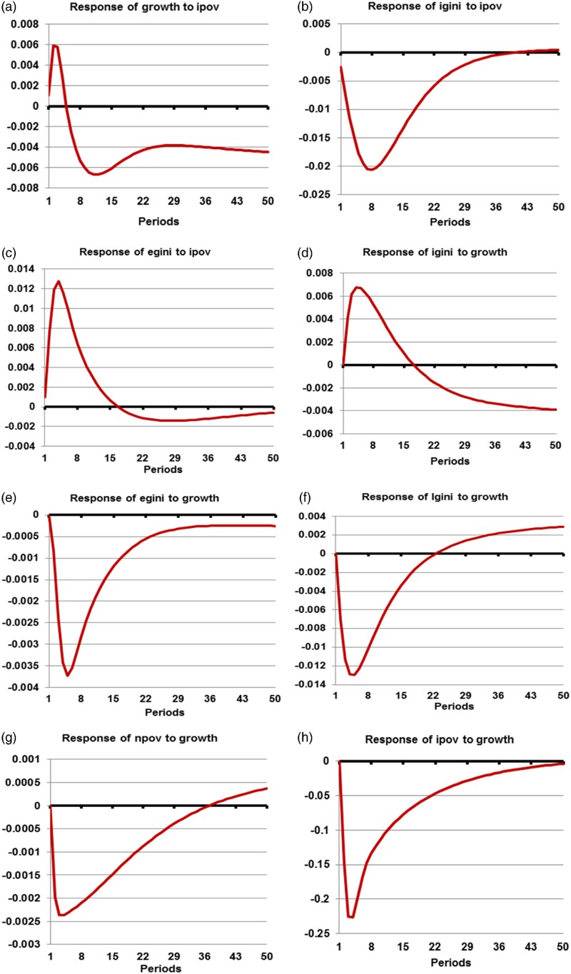
The study focused on the short-term to long-term (50-year period) effects of exogenous shocks, with the assumption that in the long-run the economy will return to equilibrium. Figure 3 shows the periodic responses of real GDP growth, income poverty, non-income poverty, income inequality, education inequality and land inequality to a one standard deviation shock in the explanatory variable confirmed to have been driving it.

From Figure 3(a), it is clear that a one standard deviation positive shock in income poverty (rising poverty level) will not have the desired effects on real GDP growth in the short term. Growth in real GDP will continue to be positive in the first four years of the shock and thereafter there will be a permanent decline in real GDP growth. Cumulatively, the positive shock in income poverty will lead to a decline in real GDP. With this shock, income inequality (Figure 3(b)) will decline permanently in the long run. The rising income poverty level will cause education inequality (Figure 3(c)) to peak in the fourth period and thereafter it will still rise, but at a decreasing rate, until the 16th period.

The effect of a positive shock in real GDP growth will continue to increase income inequality within the society for about 16 periods but will reach a peak in period three (Figure 3(d)). The positive effect of growth on income inequality will start to materialise slowly at the 18th period. This confirms the Kuznet hypothesis described earlier. However, the responses of education inequality, land inequality, income poverty and non-income poverty to positive shock in real GDP growth will remain positive in most of the periods. Higher growth in real GDP will cause education inequality (Figure 3(e)) and income poverty (Figure 3(h)) to decline permanently; land inequality (Figure 3(f)) will continue to fall until the 22nd period; and the decline in the level of human poverty (Figure 3(g)) will take a longer period to return to equilibrium. However, the response of income poverty to shock in growth recorded the biggest magnitude.

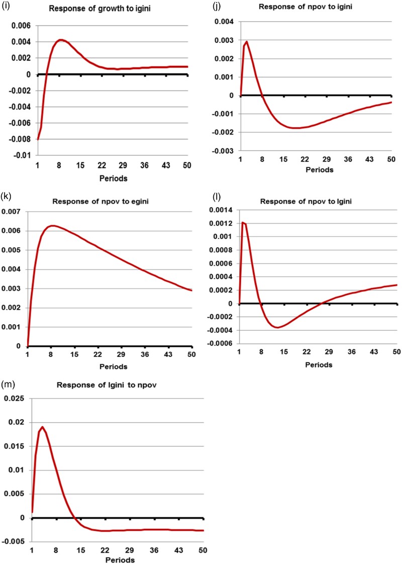
A one standard deviation positive shock in income inequality (rising income inequality) will initially lead to a fall in real GDP growth; thereafter, the effect of the shock will keep real GDP growth at a positive pace (Figure 3(i)). The effect of the shock will remain negative on non-income poverty in the short-term to medium-term (Figure 3(j)). Non-income poverty will rise in the initial eight years of the shock and thereafter begin to fall. The cumulative impact of the shock in the long run will be positive growth in real GDP and falling non-income poverty.

The response of non-income poverty to positive shock in education inequality (Figure 3(k)) and land inequality (Figure 3(l)) will remain positive over the cumulative periods of 50 years. A one standard deviation positive shock in education inequality (rising education inequality) will lead to a permanent increase in non-income poverty, while a one standard deviation positive shock in land inequality (rising land inequality) will in the initial eight periods lead to rising non-income poverty; thereafter, it will fall between the eighth and 25th periods. The cumulative impact of a one standard deviation positive shock in non-income poverty will cause land inequality to rise in the long run. The increasing land inequality was recorded in the initial 13th period of the shock (Figure 3(m)).

4. Conclusion and policy implications

In this study, the long-run relationship and the causality effects that exist between growth, poverty and inequality in South Africa (which could also be applicable to other regions of the world) were empirically established. The analysis was carried out on a panel of nine South African provinces from 1995 to 2012. In order to capture poverty and inequality in a broader context, the two measures (income and non-income) of poverty and three measures (income, education and land) of inequality were adopted for the study.

The stylised facts presented show a serious structural constraint embedded within the economy. The growth in the South African economy has only been able to translate into a small reduction in poverty but, at the same time, resulted in a resiliently high level of inequality. The panel stationary tests that were performed suggested the existence of unit roots in most of the data and this outcome justified the decision to carry out cointegration tests. The cointegration tests confirmed the existence of a long-run relationship between growth, poverty and inequality for all of the different measures that were used. At the same time, the causality tests revealed both bidirectional and unidirectional effects.

The main findings of the study revealed the following. First, the relationship between growth and income poverty was found to be bidirectional, while the relationship between growth and non-income poverty was found to be unidirectional. Whilst growth can lead to a reduction in income poverty and vice versa, the growth elasticity of income poverty was found to be larger than the income poverty elasticity of growth. The importance of a sustainable growth path was also clear from the unidirectional causality effect of rising economic growth which led to a reduction in non-income poverty.

Second, with regard to growth and inequality, there was bidirectional causality between growth and income inequality but a unidirectional causality between growth and land inequality and between growth and education inequality. Growth was found not to promote equal distribution of income in the society, but as income distribution began to equalise, economic growth picked up. This sort of relationship can be regarded as a growth–inequality disconnect. However, the unidirectional causality ran from growth, causing education and land inequality; a rising level of growth will lead to a reduction in both education and land inequality. However, the growth elasticity of land was larger than the growth elasticity of education.

Third, the causal relationship between the different measures of poverty and inequality was found to be unidirectional, except for the causality between land inequality and non-income poverty – which was found to be bidirectional. There was no causality between land inequality and income poverty. The unidirectional causality ran from income poverty to income and education inequality. However, a rising level of income poverty can lead to falling income inequality in the society. This strongly suggest that even in the midst of a rising income poverty level, equality in income can still be achieved if the little wealth that is available is shared equally among the populace. However, rising income poverty could hinder the majority of the populace from accessing education facilities. Another unidirectional causality ran from income and education inequality to non-income poverty. When income inequality increases, non-income poverty declines – implying that in the midst of rising income inequality, lower human poverty can still be achieved if the necessities of life are adequately provided. However, rising education inequality will continue to deepen human poverty within the society. The bidirectional causality between land inequality and non-income poverty revealed that improvement in land distribution can lead to a reduction in non-income poverty and vice versa, but the human poverty elasticity of land inequality was found to be larger than the land inequality elasticity of human poverty.

Finally, from the policy perspective, in order to achieve a significant reduction in poverty and inequality, policies that will promote sustainable pro-poor economic growth should remain the target of policy-makers. At the same time, policies to raise the income level of an average household and that will evenly distribute both wealth and human capital are equally important in accelerating growth to the required level needed in the economy.

Future studies should take note of the major limitations of this study. Availability of quality data will surely improve the parameter estimates found from the study.

Disclosure statement

No potential conflict of interest was reported by the author.

Notes

¹See Section 2.3 on data analysis for a detailed explanation of how the different measures of poverty and inequality are derived.

²See Appendix A (Figure A1) for provincial disaggregation of all the series.

³Education and land inequality were adopted as the preferred non-income inequality since these two factors remain at the forefront of policy debate in South Africa and have been identified as the major constraints hindering the development of the country.

⁴Detailed explanations on the derivation of income and non-income poverty can be found in Akanbi (2015). These methods were strictly adopted for data from the nine South African provinces.

Appendix A

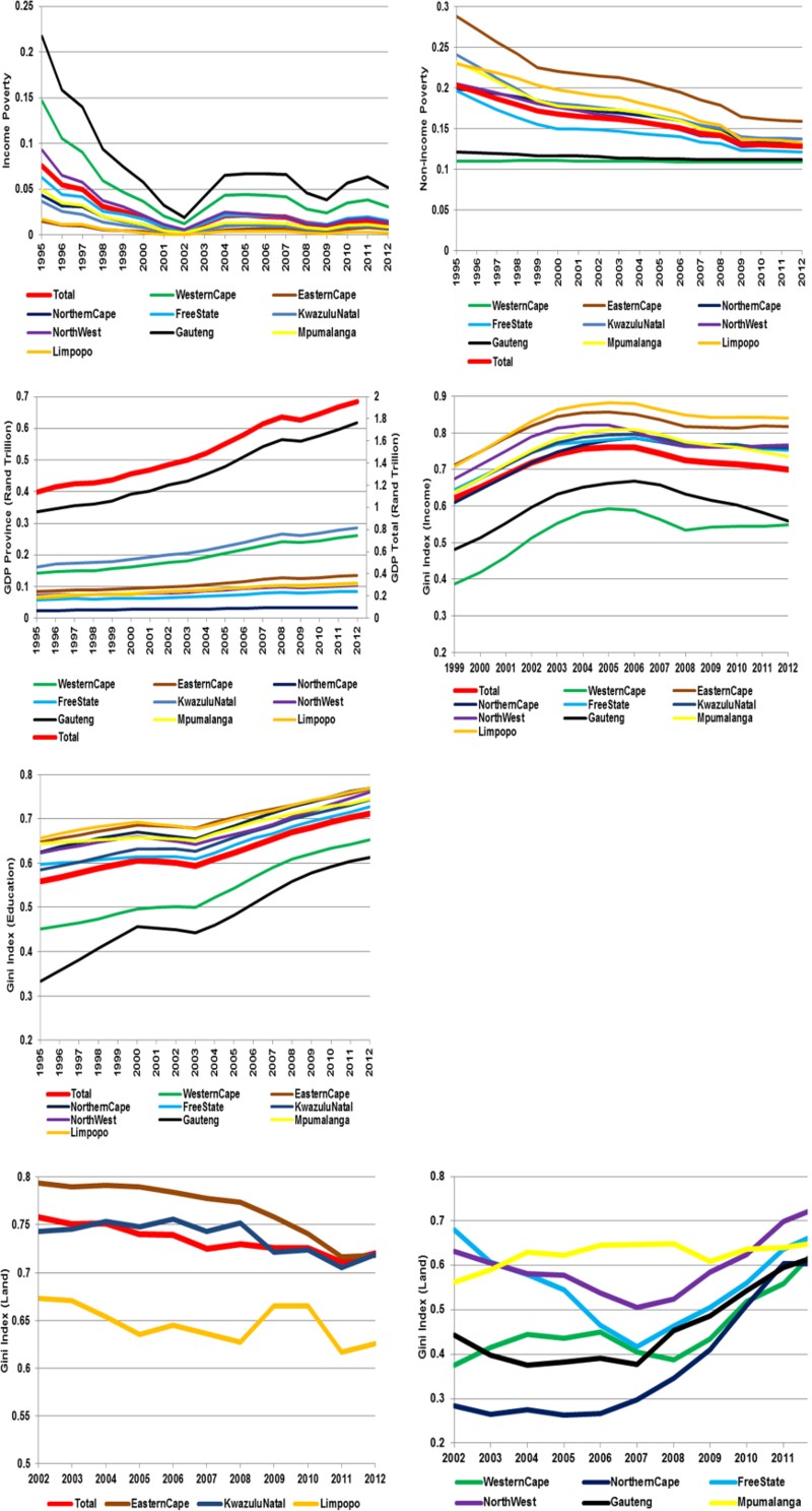
Figure A1. Total economy and provincial GDP, poverty and inequality levels Source: South African Reserve Bank, Statistic South Africa via Quantec EasyData database, World Bank Databank, African Development Indicators.

References

- Adams Jr, RH, 2004. Economic growth, inequality and poverty: Estimating the growth elasticity of poverty. World Development 32(12), 1989–2014. doi: 10.1016/j.worlddev.2004.08.006
- Adams Jr, RH & Page, J, 2003. Poverty, inequality and growth in selected Middle East and North Africa countries, 1980–2000. World Development 31(2), 2027–48. doi: 10.1016/j.worlddev.2003.04.004
- Akanbi, OA, 2015. Structural and institutional determinants of poverty in Sub-Saharan African countries. Journal of Human Development and Capabilities 16(1), 122–41. doi: 10.1080/19452829.2014.985197
- Akanbi, OA & Du Toit, CB, 2011. Macro-econometric modelling for the Nigerian economy: A growth-poverty gap analysis. Economic Modelling 28(12), 335–50. doi: 10.1016/j.econmod.2010.08.015
- Alesina, A & Rodrik, D, 1994. Distributive politics and economic growth. The Quarterly Journal of Economics 109(2), 465–90. doi: 10.2307/2118470
- Balakrishnan, R, Steinberg, C & Syed, M, 2013. The elusive quest for inclusive growth: Growth, poverty, and inequality in Asia. International Monetary Fund Working Paper 152.
- Benson, RA, 1970. Gini ratios: Some considerations affecting their interpretation. American Journal of Agricultural Economics 52(3), 444–47. doi: 10.2307/1237398
- Bhorat, H & Van der Westhuizen, C, 2007. Economic growth, poverty and inequality in South Africa: The first decade of democracy. http://scholar.google.co.za/scholar?cluster=4023147327064438921&hl=en&as_sdt=0,5&as_vis=1
- Bhorat, H, Van Der Westhuizen, C, Jacobs, T, 2009. Income and non-income inequality in post-apartheid South Africa: What are the drivers and possible policy interventions? Available online at: http://www.tips.org.za/files/income_and_non-income_inequality_in_post-apartheid_south_africa_-_bhorat_van_der_westhuizen_jacobs.pdf
- Bourguignon, F, 2003. The poverty-growth-inequality triangle, in Poverty, inequality and growth. Proceedings of the AFD-EUDN Conference 2003, 69–111.
- Datt, G & Ravallion, M, 1992. Growth and redistribution components of changes in poverty measures: A decomposition with applications to Brazil and India in the 1980s. Journal of Development Economics 38 (2), 275–95. doi: 10.1016/0304-3878(92)90001-P
- Deininger, K & Squire, L, 1996. A new dataset measuring income inequality. World Bank Economic Review 10(3), 565–91. doi: 10.1093/wber/10.3.565
- Dollar, D & Kraay, A, 2002. Growth is good for the poor. Journal of Economic Growth 7(3), 195–225. doi: 10.1023/A:1020139631000
- Dumitrescu, E & Hurlin, C, 2012. Testing for granger non-causality in heterogeneous panels. Economic Modelling 29, 1450–60. doi: 10.1016/j.econmod.2012.02.014
- Enders, W, 2004. Applied econometric time series. 2nd edn, Wiley, New York.
- Fisher, RA, 1932. Statistical methods for research workers. 4th edn, Oliver & Boyd, Edinburgh.
- Foster, J, Greer, J & Thorbecke, E, 1984. A class of decomposable poverty measures. Econometrica 52(3), 761–66. doi: 10.2307/1913475
- Ghani, E, Iyer, L & Mishra, S, 2012. The poor half billion in South Asia: Is there hope for change? voxEu.org, 9 March.
- Heshmati, A, 2004. Growth, inequality and poverty relationships. IZA Discussion paper No. 1277.
- Im, KS, Pesaran, MH & Shin, Y, 2003. Testing for unit roots in heterogeneous panels. Journal of Econometrics 115, 53–74. doi: 10.1016/S0304-4076(03)00092-7
- Johansen, S, 1988. Statistical analysis of cointegration vectors. Journal of Economic Dynamic and Control 12, 231–54. doi: 10.1016/0165-1889(88)90041-3
- Kakwani, N, 1993. Poverty and economic growth with application to cote d'Ivoire. Review of Income and Wealth 39(2), 121–39. doi: 10.1111/j.1475-4991.1993.tb00443.x
- Kanbur, R, 2005. Growth, inequality and poverty: Some hard questions. Journal of International Affairs 58(2), 223–32.
- Khan, MH, 2009. Governance, growth and poverty reduction. DESA Working Paper No. 75.
- Kraay, A, 2006. When is growth pro-poor? Evidence from a panel of countries. Journal of Development Economics 80, 198–227. doi: 10.1016/j.jdeveco.2005.02.004
- Kuznets, S, 1955. Economic growth and income inequality. American Economic Review 45(1), 1–28.
- Leibbrandt, M, Woolard, I & Bhorat, H, 2001. Understanding contemporary household inequality in South Africa. In Fighting poverty: Labour markets and inequality in South Africa. HSRC Press, Cape Town, 21–40.
- Leibbrandt, M, Poswell, L, Naidoo, P & Welch, M, 2006. Measuring recent changes in South African inequality and poverty using 1996 and 2001 census data. In Kanbur, R & Bhorat, H (Eds.), Poverty and policy in post-apartheid South Africa. HSRC Press, Cape Town.
- Levin, A, Lin, CF & Chu, CSJ, 2002. Unit root test in panel data: Asymptotic and finite sample properties. Journal of Econometrics 108, 1–24. doi: 10.1016/S0304-4076(01)00098-7
- Maddala, GS & Wu, S, 1999. A comparative study of unit root tests with panel data and a new simple test. Oxford Bulletin of Economics and Statistics, 61(Special Issue), 631–52. doi: 10.1111/1468-0084.61.s1.13
- ODI (Overseas Development Institute), 2002. Inequality briefing: Why inequality matters for poverty. Briefing Paper No. 2.
- Person, T & Tabellini, G, 1994. Is inequality harmful for growth? American Economic Review 84(3), 600–21.
- Ravallion, M, 1997. Can high-inequality developing countries escape absolute poverty? Economics Letters 56, 51–7. doi: 10.1016/S0165-1765(97)00117-1
- Ravallion, M, 2001. Growth, inequality and poverty: Looking beyond averages. World Development 29, 1803–15. doi: 10.1016/S0305-750X(01)00072-9
- Ravallion, M, 2012. Why don't we see poverty convergence? American Economic Review 102(1), 504–23. doi: 10.1257/aer.102.1.504
- Ravallion, M & Chen, S, 1997. What can new survey data tell us about recent changes in distribution and poverty? The World Bank Economic Review 11(2), 357–82. doi: 10.1093/wber/11.2.357
- Roine, J, Vlachos, J & Waldenstrom, D, 2009. The long-run determinants of inequality: What can we learn from top income data? http://www.anst.uu.se/h/danwa175/Research_files/The%20LongRun%20Determinants%20of%20Inequality%20%20What%20Can%20We%20Learn%20from%20Top%20Income%20Data.pdf
- Saad-Filho, A, 2010. Growth, poverty and inequality: From Washington consensus to inclusive growth. DESA Working Paper No. 100.
- Slack, B & Rodrigue, JP, 2009. The Gini coefficient, in the geography of transport equipment. Routledge, New York.
- UNDP (United Nations Development Programme), 1997. Human Development Report 1997. Oxford University Press, New York.
- Van Der Berg, S, 2010. Current poverty and income distribution in the context of South African history. University of Stellenbosch Economic Working Papers: 22/10.
- Wu, S, 1998. Nonstationary panel data analysis. Thesis, Ohio State University.