Economy-wide implications of biofuel production in Zambia

ABSTRACT

Potential biofuel demand in South Africa is estimated to increase to 1550 million litres by 2025 due to mandatory blending rates. Land and water constraints, however, limit the ability for domestic production. Zambia, due to its abundance in land, suitable climate, supportive set of bioenergy incentives and close geographical location to South Africa, has the potential to meet this increase in demand. Using a dynamic recursive computable general equilibrium model, we estimate the macro- and socio-economic impacts of bioethanol production in Zambia from three potential crops: sugarcane, cassava and sweet sorghum. The results show that the development of a single product bioethanol industry has the potential to increase economic growth without negatively affecting overall food security. Further expansion of the industry to multiple products results in larger gains to growth and welfare.

KEYWORDS:

• Biofuels
• computable general equilibrium
• food security
• Zambia

JEL CODES:

• Q16
• C68
• Q18

1. Introduction

Global biofuel demand has increased significantly over the past decade as countries implemented fuel blending mandates and targets as mitigation strategies to reduce greenhouse gas emissions in the transport sector. Between 2005 and 2015, biofuel production increased from less than 50 billion to over 130 billion litres, accounting for about 4% of global road transport fuel use (IEA, 2016). Demand is expected to increase to 200 billion litres by 2025 (IEA, 2016) as more countries mandate the use of biofuels for transportation.

Blending mandates have also increasingly been implemented in Africa, with many countries in the Southern African Development Community already having mandates or targets in place. This includes South Africa, who in 2014 announced blending rates of between 2% and 10% for bioethanol and 5% for biodiesel. Under a low growth scenario, South African bioethanol (under a 10% mandate) and biodiesel demand is therefore projected to rise to 1400 and 90 million litres, respectively, by 2025 (Stone et al., 2015). Demand could be twice as large if flexible fuel cars are used. The South African market could therefore serve as a key anchor market for biofuel production and the development of a biofuel market in the southern African region.

Zambia can become a large supplier of bioethanol. Its near-central geographical location, suitable climate, abundance in land and (on paper) supportive set of bioenergy incentives provide a strong case for successful production within the country. Identified potential bioethanol crops, namely sugarcane and cassava, are also well established with large volumes currently produced for own consumption and foreign markets (Samboko et al., 2017a). The potential of biofuel production to assist developing countries in meeting their development goals (FAO, 2013; Ferede et al., 2013), including poverty reduction, provides further argument for the development of such an industry in Zambia. In 2010, about 60% of the Zambian population, which is highly dependent on the agriculture sector for employment, was living below the national poverty line (World Bank, 2010).

In this paper, we estimate the potential economic impacts of developing a bioethanol industry in Zambia using a dynamic computable general equilibrium (DCGE) model. This study follows a similar approach to that of Arndt et al. (2010; 2012), Thurlow et al. (2016) and Schuenemann et al. (2017) and is based on the work by Hartley et al. (2017). Three potential crops (i.e. sugarcane, cassava and sweet sorghum) under different farming models are considered, accounting for country specific constraints such as land and resource availability. Given concerns around food security in the commercial crop use debate (Shumba et al., 2009), we also assess the impact of bioethanol production on representative household groups’ food consumption. Furthermore, we assess the potential of extending the single product bioethanol industry into a multi-product industry by including the production of electricity through bagasse cogeneration for the case of sugarcane.

Section 2 of this paper discusses the potential for biofuel production in Zambia and presents estimated costs of feedstock and ethanol production. Section 3 describes the DCGE model, scenarios and assumptions. Section 4 reports the model results, and section 5 concludes.

2. Potential for biofuel production in Zambia

2.1. Feedstock crops and resource availability

Samboko et al. (2017a) identifies several potential crops for ethanol use in Zambia; these include sugarcane, agave, sweet sorghum, maize, cassava, pineapples and sweet potatoes. Sugarcane and cassava are, however, highlighted as two key crops to consider, given the large quantities currently produced in the country. In 2014, Zambia produced around 4 043 000 and 919 000 metric tonnes (MT) of sugarcane and cassava, respectively (FAOSTAT, 2014).

2.1.1. Sugarcane

Sugarcane in Zambia is primarily grown on irrigated commercial farms owned by sugar-producing companies. Commercially farmed sugarcane accounts for 60% of total supply in the country and uses about 23 000 hectares (Ha) of land. The remaining 40% of supply is produced by around 400 smallholder farmers through outgrower schemes, specifically the Sugarcane (commercial), cassava and sweet sorghum production costs are calculated using data from Sinkala et al. (2013), Sinkala (personal communication, Prof. Thomson Sinkala, 24 May 2016) as well as enterprise budget data collected by Samboko et al. (2017a), respectively. Due to a lack of data, we estimate smallholder costs by applying commercial- to-smallholder budget ratios from a similar study for Tanzania (Arndt et al., 2012) to commercial budgets. Expenditure on seed in sugarcane production from Sinkala et al. (2013) has been amended as suggested by the Indaba Agricultural Policy Research Institute to reflect average annual expenditure. Calculated bio-crop costs range between US$0.2 and US$0.3 per litre (/L) (see Table 2). Cassava is found to be the cheapest bio-crop, costing 30% less than sugarcane and 20% less than sweet sorghum. The lower cost is driven by the relatively lower expenditure on intermediate inputs, including fertiliser which is not used in cassava farming. Cassava farmers spend a larger share of their budget on factor returns (i.e. payment to land, labour and capital). Factor payments account for almost 80% of total expenditure relative to 40% and 55% under sugarcane and sweet sorghum. Increased cassava production would therefore have larger gross value-added (GVA) impacts per unit of output than sweet sorghum or sugarcane, while the latter has stronger links with the rest of the economy. Smallholder farms are more labour intensive than commercial farms, with returns to labour accounting for almost 25% of smallholder sugarcane expenditures and only 10% of commercial farming budgets. Cassava and sweet sorghum are also labour intensive, with 40% of expenditure spent on wages. Commercial sugarcane farmers spend almost 30% of their budgets on returns to capital. Interestingly, cassava farmers also spend a relatively large share of the budget on payments to capital. Kaleya Smallholder Company, Maggobo and Manyoyo schemes. Smallholder sugarcane output is currently sold to sugar-producing companies, primarily Zambia Sugar Plc (Chisanga et al., 2014; Kalinda & Chisanga, 2014). As a result, these farming activities are also irrigated as smallholder farmers receive water supply from core estates as part of the services provided through the outgrower schemes. Average yields of smallholder farmers are reported to compare favourably to commercial farmers, reaching up to 110 to 115 MT/Ha (Bangwe & van Koppen, 2012). Keyser (2007) has identified the sugar cane value chain as the most profitable involving smallholder farmers in Zambia, highlighting the sector’s links to the local economy and its importance in poverty reduction.

2.1.2. Cassava

Cassava is a low-input, drought tolerant crop primarily grown by smallholder farmers located in the Luapula and Northern provinces of Zambia. Commercial farming accounts for less than 1% of total output. Currently cassava is largely used as a staple crop, second only to maize, with smaller shares used as an intermediate input into the manufacturing sector (FSRP and ACF, 2010). Average cassava farming yields vary depending on the variety grown. Sitko et al. (2011) report fresh root cassava farm yields of 3.5 MT/Ha when using traditional cassava varieties and between 6 and 12 MT/Ha for new varieties. Potential cassava yields from research studies have ranged between 7 MT/Ha in the case of local varieties and 22 to 41 MT/Ha for new varieties. Estimates from the Food Security Research Project and the Agricultural Consultative Forum (FSRP and ACF, 2010) have recorded higher on-farm yields of between 18 and 20 MT/Ha. The Zambian Ministry of Agriculture estimates current yields at around 11 MT/Ha.

2.1.3. Sweet sorghum

Sweet sorghum provides an alternative bio-crop to sugarcane and cassava. It can be grown more than once a year; has low input requirements; is drought tolerant; and is a dual-purpose crop, meaning that it can be used for both bioethanol and food production. Sweet sorghum is currently produced in small quantities, around 11 000 MT in 2014 (FAOSTAT, 2014), by smallholder farmers and is rainfed. Current sweet sorghum yields are reported to be between 30 and 40 MT/Ha. More recent versions of the crop under study at the University of Zambia, however, display the potential to substantially reduce the costs of bioethanol production because of higher yields per Ha (Samboko et al., 2017a). The three varieties under study at the university recorded yields of between 70 and 83 MT/Ha under research conditions which included fertiliser use as well as supplemental irrigation prior to rains. More recent yields recorded were comparable to that of sugarcane at 100 MT/Ha.

2.1.4. Land and water

Samboko et al. (2017b) estimate that only 14% of the 40 million Ha of land available for agricultural purposes is currently used, with less than 6% of the 2.75 million Ha of land with irrigation potential utilised. Furthermore, they find that the land available aligns well with areas receiving sufficient water supply for bio-crop production.

The volume of land required for bioethanol production is dependent on the crop’s achievable yields and bioethanol conversion rate. This differs across crops. Using reported values (see Table 1) it is estimated that about 180 000 Ha of land is required for sugarcane production to supply the South African bioethanol demand of 1400 million litres. Due to lower crop yields, more land is required in the case of cassava and sweet sorghum (i.e. 381 000 and 784 000 Ha). These land demands are well within the available land supply.

Table 1. Summary of crop yields in Zambia.

	Zambia: Estimated yields (MT) per ha^a
	Small-scale farmers			Small-scale high yielding farmers		Large-scale farmers
	Sugarcane	Sweet sorghum	Fresh root cassava	Sweet sorghum	Fresh root cassava	Sugarcane
Yield (mt/ha)
Shumba et. al (2009)	112-120	30-40	-	40-60
Bangwe & van Koppen (2012)	110-115	-	-	-	-	-
Sitko et al. (2011)	-	-	3.5 -12	-	-	-
	-	-	7 - 41	-	-	-
Sinkala et al. (2013)	-	-	-	-	-	110
Tembo & Sitko (2013)	-	-	2.85	-	-	-
Sinkala (personal communication, Prof. Thomson Sinkala, 24 May 2016)	-	-	11	-	-	-
Samboko et al. (2017a)	-	-	5.87	-	13.79	-
	-	-	-	70.2-82.5	-	-
Ethanol conversion rate (litre/mt)
Shumba et. al (2011)	80	55	-	55	-	80
Sinkala et al. (2013)	80	45	200	45	200	80
Sinkala (personal communication, Prof. Thomson Sinkala, 14 November 2016)	-	-	167	-	167	-
Samboko et al. (2016)	-	51	-	51	-	-
Water requirement (mm)^b	1,500-2,500	450-700	400-750	450-700	400-750	1,500-2,500

^a Italics indicate yield estimates under research condition

^b Sinkala et al. (2013)

Cassava and sweet sorghum require between 450 and 700–750 mm of water. Average rainfall in areas with land availability ranges between 800 and 1500 mm (Samboko et al., 2017a), which is sufficient to meet the demands of these crops. Sugarcane requires more water, between 1500 and 2500 mm; however, the crop is irrigated.

The most recent estimates of crop yields and conversion rates are used in this analysis. In the case of yields the following are assumed: commercial sugarcane – 110 MT/Ha; smallholder cassava – 22 MT/Ha; smallholder sweet sorghum – 35 MT/Ha. In the case of smallholder sugarcane farming we assume a yield of 70 MT/Ha due to estimates of production costs (see section 2.2.1). Conversion rates of 80, 167 and 51 are used for sugarcane, cassava and sweet sorghum.

2.2. Costs of bioethanol production

2.2.1. Bioethanol crop farming

Sugarcane (commercial), cassava and sweet sorghum production costs are calculated using data from Sinkala et al. (2013), Sinkala (personal communication, Prof. Thomson Sinkala, 24 May 2016) as well as enterprise budget data collected by Samboko et al. (2017a), respectively. Due to a lack of data, we estimate smallholder costs by applying commercial- to-smallholder budget ratios from a similar study for Tanzania (Arndt et al., 2012) to commercial budgets. Expenditure on seed in sugarcane production from Sinkala et al. (2013) has been amended as suggested by the Indaba Agricultural Policy Research Institute to reflect average annual expenditure. Calculated bio-crop costs range between US$0.2 and US$0.3 per litre (/L) (see Table 2). Cassava is found to be the cheapest bio-crop, costing 30% less than sugarcane and 20% less than sweet sorghum. The lower cost is driven by the relatively lower expenditure on intermediate inputs, including fertiliser which is not used in cassava farming. Cassava farmers spend a larger share of their budget on factor returns (i.e. payment to land, labour and capital). Factor payments account for almost 80% of total expenditure relative to 40% and 55% under sugarcane and sweet sorghum. Increased cassava production would therefore have larger gross value-added (GVA) impacts per unit of output than sweet sorghum or sugarcane, while the latter has stronger links with the rest of the economy. Smallholder farms are more labour intensive than commercial farms, with returns to labour accounting for almost 25% of smallholder sugarcane expenditures and only 10% of commercial farming budgets. Cassava and sweet sorghum are also labour intensive, with 40% of expenditure spent on wages. Commercial sugarcane farmers spend almost 30% of their budgets on returns to capital. Interestingly, cassava farmers also spend a relatively large share of the budget on payments to capital.

Table 3. Bioethanol production costs by crop, US$ per litre (2016 prices).

	Large-scale feedstock farms	Small-scale feedstock farms
	Sugarcane	Sugarcane	Sweet sorghum	Cassava
Feedstock unit costs	0.304	0.303	0.261	0.209
Capital cost and interest	0.000	0.000	0.000	0.057
Chemicals/enzymes	0.057	0.057	0.057	0.019
Energy/utility	0.019	0.019	0.019	0.085
Operations/maintenance	0.038	0.038	0.038	0.028
Unforseen	0.019	0.019	0.019	0.019
Total cost	0.436	0.435	0.394	0.417

Source: Own calculations; Sinkala et al. (2013)

Table 2. Feedstock production costs by crop, US$/Ha (2016 prices).

	Large-scale farmers			Small-scale farmers
	Sugarcane	Sweet Sorghum	Cassava	Sugarcane	Sweet sorghum	Cassava
Seed	181.6			181.6	7.3	45.0
Chemicals	860.3			749.2	141.3	-
Food						3.0
Wood and paper					8.3
Business services	311.3			124.6	30.1	42.2
Financial services	40.8			45.4		30.0
Trade services	95.3			37.8		-
Transport	116.5			116.5	23.1	40.0
Labour	257.9			460.2	170.8	278.0
Land	95.8			21.9	19.6	123.5
Capital	718.4			200.1	66.0	205.9
Total cost	2,677.9			1,937.5	466.6	767.5
mt/ha	110.0			80.0	35.0	22.0
lires/ha	8,800.0			6,400.0	1,785.0	3,674.0
Total cost per litre	0.304			0.303	0.261	0.209

Source: Own calculations; Sinkala et al. (2013); Sinkala (personal communication, Prof. Thomson Sinkala, 24 May 2016); and Samboko et al. (2016)

2.2.2. Bioethanol processing

No commercial production of bioethanol takes place in Zambia (Samboko et al., 2017a). As a result, there are no Zambia-specific data available for bioethanol processing. Sinkala et al. (2013) estimate bioethanol processing costs for Zambia from a 2010 study by the Asia Pacific Economic Cooperation (APEC, 2010). These costs are included in this study and presented in Table 3 and include the feedstock costs shown in Table 2. The production cost of bioethanol in Zambia is calculated to be between US$0.39/L and US$0.44/L depending on the feedstock crop chosen. Sweet sorghum derived bioethanol has the lowest factory gate price. The price of ethanol from cassava is about US$0.02 higher due to higher ‘non-feedstock’ processing costs. ‘Non-feedstock’ cassava ethanol processing costs are about 57% higher than sweet sorghum and sugarcane because of larger initial investment costs as well as higher utility costs. Bangwe & van Koppen (2012) estimate that crop yields by smallholder sugarcane farmers average 110 MT/Ha. This is higher than our assumed yield of 70 MT/Ha. If yield estimates by Bangwe & van Koppen (2012) are realised, the price of ethanol produced using smallholder sugarcane would decrease to US$0.35/L. Similarly, higher yields for sweet sorghum as experienced under the University of Zambia’s research programme would lead to lower bioethanol prices of only US$0.24/L (based on a yield of 82.5 MT/Ha). These are competitive with factory gate prices estimated for Mozambique (Hartley et al., 2016).

3. Modelling methodology

3.1. Model

A DCGE model for Zambia is used in this study. It is based on the generic static and dynamic models described in Lofgren et al. (2002) and Diao & Thurlow (2012) and is a descendant of the class of computable general equilibrium (CGE) models introduced by Dervis et al. (1982). It uses a 2007 Social Accounting Matrix (SAM) (Chikuba et al., 2013) consisting of 44 industries and commodities, 4 labour groups and 5 rural and urban household groups. Households are further grouped by income quintile. Labour categories are defined by education levels (i.e. incomplete and complete primary; completed secondary; completed tertiary). Other institutions (i.e. government, enterprises and the rest of the world) are also represented.

Behavioural equations capture the decision-making process of industries and households who maximise profits and utility subject to costs and purchasing power, respectively. Producers consume both domestic and imported intermediate goods and services as well as production factors (i.e. capital, labour and land). Intermediate consumption behaviour is governed by Leontief functions, while constant elasticity of substitution functions dictates production factor consumption behaviour. As a result, fixed shares of intermediate goods and services are required in production, but production factors can be substituted according to changes in relative prices.

We assume that each activity only produces one commodity which is sold to other industries as intermediate inputs or to households, government and the rest of the world for final consumption. The quantity of commodities provided to domestic versus international markets is based on relative prices and is governed by constant elasticity of transformation functions. Similarly, the volume of imports is based on relative prices and is governed by Armington functions. Global prices remain fixed as the Zambian economy is too small to directly affect them.

Households earn an income from providing labour, land and capital assets to industries and from government and foreign transfers. Returns to foreign labour, land and capital are repatriated. Households consume both domestic and foreign commodities, pay taxes, transfer money abroad and save. Consumption is based on a linear expenditure system of demand.

Structural equations ensure macro-economic consistency between incomes and expenditures within the model. Closure rules are used to describe the functioning of the economy; these include the behaviour of exchange rates, investment, government savings, prices and production factors supplies. In this paper, we assume that the exchange rate adjusts to absorb shocks to the economy, while foreign savings remains fixed. The level of investment is determined by total savings (i.e. private, government and foreign). Government savings adjust for changes in its income and expenditure – tax rates remain unchanged. The domestic price index is used as the model numeraire. To fully assess the impact on resource shifts, we assume that all labour and land in the economy is initially fully employed. Capital (non-biofuel) is also fully employed but cannot shift to other sectors.

3.2. Structure of the Zambian economy

In 2007, the agriculture sector accounted for 13.8% of real GDP and 8.2% of total exports. The sector employed 71.3% of the total workforce, primary low skilled workers, but only accounted for 16.3% of labour income. More than 90% of food demand is satisfied by domestic production.

Mining is the main earner of foreign income, followed by manufacturing (largely metal products and machinery). Food processing was the largest manufacturing sub-sector and accounted for 5% of total real GDP. The services sector comprised the largest share of GDP primarily due to the wholesale and retail trade services sub-sector (Table 4).

Table 4. Structure of Zambia’s economy, 2007.

	Share of total (%)
	GDP	Labour income	Employment	Exports	Imports	Exports/output (%)	Imports/demand (%)
Total GDP	100.0	100.0	100.0	100.0	100.0	12.0	16.4
Agriculture, forestry and fishing	20.0	16.7	71.3	8.6	1.5	5.4	1.3
Food crops	10.2	4.3	18.5	3.9	0.6	6.3	1.4
Other agriculture	3.6	4.5	19.2	4.3	0.6	16.8	3.8
Forestry and fishing	6.2	7.9	33.6	0.0	0.0	0.0	0.0
Mining	4.9	2.0	2.0	71.4	0.0	89.6	0.0
Manufacturing	9.7	6.1	3.5	10.5	77.7	5.0	40.3
Food processing	5.8	4.0	2.2	5.0	4.6	4.5	5.8
Other manufacturing	3.9	2.1	1.2	5.6	73.1	5.8	63.2
Other industries	15.2	13.8	2.0	0.4	0.3	0.4	0.3
Services	50.2	61.3	21.2	9.5	20.8	3.3	6.9

Source: 2007 Zambia SAM, CSO (2011).

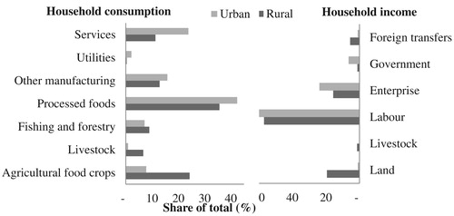
Food consumption makes up the largest share of rural (42%) and urban (35%) household expenditure in Zambia. Processed foods make up the largest share of urban household diets (about 85%), with agricultural food crop consumption comprising mainly horticulture crops. While rural households spend a significant share of their budgets on processed foods, they also spend a relatively large share of their budgets on agricultural food crops, primarily cassava and maize.

Household incomes are primarily derived from the provision of labour. Wage income accounts for 68% and 57% of total urban and rural income, respectively; however, 72% of total labour returns are paid to urban households. Urban households also receive a relatively large share of their incomes from capital returns (24%) and government transfers (6%). Rural household incomes are more diverse, with returns to land and capital as well as foreign transfers constituting around 40% of total income. Capital returns to rural households make up only 23% of total capital returns with the remaining 77% paid to urban households (Figure 1).

Figure 1. Rural and Urban household consumption and income, 2007. Source: 2007 Zambia SAM.

3.3. Baseline growth path

The 2007 structure of the Zambian economy described above serves as the starting point for defining relationships and parameters in the DCGE model. In the baseline scenario, we extend this structure to 2025. Exogenous parameters such as labour and land supply, government expenditure and foreign savings are updated externally based on historical trends. Capital stocks are updated in each period by investment from the previous period, accounting for depreciation. Increases in sector capital stocks are a function of profitability in the previous period as well as share of total capital stock. An average total factor productivity growth rate of 0.8% per annum is assumed such that the model replicates historical and future growth. Future growth is based on the International Monetary Fund (IMF, 2016) projection of 5.1% average annual growth over 2015–25. For the purposes of this study the baseline growth rate is, however, somewhat arbitrary as our interest is in the differences between the base and various scenario outcomes.

3.4. Including the biofuel industry

The biofuel industry, which includes both bio-crop farming and ethanol processing, is included in the SAM using the technology vectors illustrated in Tables 2 and 3. In the baseline scenario, production by these sectors is set to (almost) zero so that their activity is not visible. Capital for commercial and smallholder sugarcane farming and ethanol processing is assumed to come from international markets. Returns to capital (after tax) from these sectors are repatriated using a separate and newly introduced factor account, i.e. fbio-l. Capital for non-sugarcane smallholder farming (i.e. fbio-s) is assumed to come from international donor funding; (after tax) capital returns are transferred in the same way as non-biofuel capital.

The bioethanol processing sector creates a demand for feedstock crops. To simulate the expansion in ethanol production, we exogenously increase the supply of land given to feedstock farmers for the specific scenario. Farmers draw in capital, labour and intermediate inputs through their production processes. Feedstock outputs are used by the processing sector, along with capital, labour and intermediate inputs, to produce bioethanol.

Bioethanol processing can also lead to increased supply of non-biofuel commodities through the development of by-product activities. Examples of by-products from bioethanol production include electricity through cogeneration as well as animal feed. Sugarcane waste (i.e. bagasse) is usually used by sugar mills for electricity production for own use at relatively little cost. In most cases, however, there is an excess supply that can be sold to the national grid. Mauritius has been very successful at this. In 2013, the country produced 475 GWh of electricity (16% of total production) from bagasse (MEPU, 2015). Deepchand (2005) estimates that, in Africa, 70–110 kWh of electricity can be produced from the waste of 1 MT of sugarcane. To illustrate the benefit of a multiple product bioethanol industry, the SAM is further adapted to include the potential for cogeneration using bagasse. The technology vector for this sector is like that of the sugarcane bioethanol processing sector but also includes the cost of capital of generating electricity. Electricity is a by-product from bioethanol production, adding to domestic supply in the country. Based on Deepchand’s (2005) estimates, we assume that 70 kWh of electricity is produced per MT of sugarcane. Since cogeneration is essentially free, the value of the electricity produced is added to the operating surplus of the bioethanol industry. As a result, this activity becomes more profitable.

We assume that all bioethanol is exported. It is likely that some of the bioethanol produced may be used domestically. This would reduce the need for imported fuel and have a positive impact on the country’s balance of payments. Samboko et al. (2017a) estimate that in 2015 bioethanol and biodiesel demand in Zambia reached around 49 million litres, respectively. Either way, this has a limited impact on the results presented here as domestic bioethanol use would reduce bioethanol exports, which would reduce the positive impact on the balance of payments. The larger positive impact from assuming no domestic consumption and hence higher exports therefore essentially accounts for the positive balance of payment impact from domestic use.

3.5. Scenarios and assumptions

We assume an annual bioethanol production target of 1400 million litres by 2025 for Zambia to satisfy the South African market. Six scenarios described in Table 5 are considered. The scenarios are designed such that the economy-wide impacts of the following can be assessed: (i) different feedstock crops; (ii) different farming models; (iii) by-products, specifically cogeneration; and (iv) land displacement.

Table 5. Scenarios.

Scenario	Description
1 Sugar – status quo	Bioethanol production using sugarcane (i.e. 60% commercial; 40% smallholder)
2 Sugar – 20:80	Bioethanol production using sugarcane (i.e. 20% commercial; 80% smallholder)
3 Sugar – status quo and cogeneration	Bioethanol and electricity production using sugarcane (i.e. 60% commercial; 40% smallholder)
4 Cassava	Bioethanol production using cassava
5 Cassava and displacement	Bioethanol production using cassava, including the cost of land displacement (50% of smallholder farming land needs)
6 Sweet sorghum	Bioethanol production using sweet sorghum

Differences between scenarios 1 and 2 assess the impact of increased smallholder farming. In scenario 2, the share of smallholder sugarcane production is increased from 40% to 80%. Commercial farmers are assumed to produce the remaining sugarcane. Because of their higher labour intensity, an increased use of smallholder farmers is expected to result in increased employment in the bioethanol industry which may result in larger welfare gains for low income households.

The impact of cogeneration is assessed in scenario 3. The production of 1400 million litres is estimated to result in approximately 1225 GWh of electricity, lowering electricity prices and therefore production costs, particularly for energy intensive sectors.

Scenarios 4 and 6 consider the impacts of alternative bioethanol feedstock crops, primarily cassava and sweet sorghum.

Scenario 5 aims to capture food security concerns by including the potential impact of land displacement. Specifically, we consider a 50% rate of smallholder land displacement (following Arndt et al., 2012) as a result of industrial cassava farming. This is not included in other scenarios as food security is generally not considered to be a major concern in Zambia. Sinkala et al. (2013) argue this as (i) an excess of productive agricultural lands is available, (ii) open-ended food prices in Zambia (and Africa in general) are more lucrative than capped prices that biofuels would offer, (iii) the biofuels industry stimulates high yield crop production approaches because of the limited radius of feedstock viability and (iv) food availability in biofuel production areas are part of the biofuels competitive advantage for the industry’s survival. Samboko et al. (2017b) agree that, apart from current limited food availability in the Western and Muchinga provinces, food security is not a major constraint in most of Zambia.

While climate variability may potentially have a significant impact on crop production yields, particularly in the case of rainfed crops such as cassava and sweet sorghum, for irrigation based sugarcane the impacts are likely to be smaller, translating rather into higher irrigation costs as increased evaporation rates would require increased irrigation frequency. These impacts would lead to higher feedstock crop prices, raising the cost of bioethanol and potentially making it less competitive relative to alternative fuels and suppliers. These impacts are not considered in this paper and provide an avenue for further analysis.

4. Results

This section reports on the modelling results. Unless specified otherwise, the results are presented as the percentage point (%pt) change in the average annual growth rate over 2015–25 relative to the baseline scenario. The ‘Total GDP’ result of 0.029 for scenario 1 is therefore interpreted as an increase in the average annual growth rate from 5.1% in the baseline to 5.129%.

4.1. Overall economic impacts

The development of a single product bioethanol industry in Zambia has a positive impact on real GDP growth which increases by 0.03–0.04%pts per annum (scenarios 1, 4 and 6). The largest gains to growth are experienced for cassava, which has the largest value added per unit of output produced. This is followed by sugarcane, with sweet sorghum reflecting the smallest gains to real GDP growth.

Expanding the bioethanol industry to include the production of by-products has the potential to amplify gains to the economy. Average annual real GDP growth increases by 0.058%pts in scenario 3 relative to 0.029%pts in scenario 1. By 2025, electricity produced from bioethanol production accounts for about 4% of total electricity demanded. The increase in electricity supply lowers electricity costs, raising profitability as well as household purchasing power. This positively affects production (particularly for energy intensive producers) and consumption.

The assumed displacement of land due to bioethanol crop production (scenario 5) lowers the gains to real GDP growth as it reduces the land resources available for other agricultural use. Non-bioethanol feedstock production declines are larger under this scenario, resulting in larger price increases which have knock-on effects on the rest of the economy. The overall impact on real GDP growth, however, remains positive with average annual real GDP growth increasing by 0.007%pts relative to the baseline.

Increasing the share of smallholder sugarcane production (scenario 2) has a marginally smaller impact on real GDP growth than using the status quo production model (scenario 1). This is because the value added of commercial sugarcane farmers is marginally larger than that of smallholder farmers. Smallholder sugarcane farmers are also more labour intensive than commercial farmers, which means that upward pressure on wages and hence production costs are larger.

The expansion of bioethanol production is simulated through an increase in land allocated to feedstock producers. Thus, land supply increases relative to the baseline scenario (see Table 6), resulting in a decrease in the return to land. As indicated in section 2.1.4, the volume of land needed for industrial crop use is 180 000, 381 000 and 784 000 Ha for sugarcane (status quo), cassava and sweet sorghum, respectively. The return per Ha of land is therefore lower in the case of cassava and sweet sorghum than in the case of sugarcane (status quo). Smallholder sugarcane farmers require more land than their commercial counterparts due to lower yields. As a result, larger land increases are experienced in scenario 2 relative to scenario 1. Scenario 5 illustrates smaller increases in annual land supply growth as 50% of the land required is assumed to come from current agricultural activities.

Table 6. Core macro-economic assumptions and results, 2015–25.

		Scenario 1	Scenario 2	Scenario 3	Scenario 4	Scenario 5	Scenario 6
	Baseline	Sugarcane, status quo	Sugarcane, 20–80	Sugarcane and cogeneration	Cassava	Cassava and displacement	Sweet sorghum
Average annual growth rate (%)
Total GDP	5.1	5.129	5.119	5.158	5.139	5.107	5.118
Labour Supply	4.0	4.000	4.000	4.000	4.000	4.000	4.000
Capital stock	4.7	4.681	4.679	4.684	4.678	4.675	4.676
Livestock stock	0.6	0.600	0.600	0.600	0.600	0.600	0.600
Land Supply	0.6	1.287	1.373	1.287	1.981	1.309	3.264
Deviation from baseline final year value, 2025 (%)
Real exchange rate*	–	0.399	0.446	0.306	0.668	1.187	0.603
Real food prices	–	0.018	0.030	0.009	0.144	1.397	0.113

*A positive (negative) value indicates an appreciation (depreciation).

Source: Authors’ calculation based on the results from the Zambia CGE model.

Labour is assumed to be fully employed. Additional labour demand from the biofuel industry results in an increase in wages as firms compete for a limited resource. This has a negative impact on sectors with price sensitive demand. These sectors reduce their production thereby releasing workers who move into the biofuel industry. The decreases in activity by these sectors constrain the positive impact of bioethanol production on real GDP but also release resources to be used elsewhere in the economy. Cassava is one sub-sector that benefits from this endogenous shift in resources. This is an important finding given the importance of cassava for food security in Zambia, particularly in rural areas.

Food prices increase because of: higher production costs, lower processed food production and increased demand from households due to higher incomes. Food price increases are larger in the case of cassava and sweet sorghum (scenario 4 and 6) as they are more labour intensive than sugarcane. The higher labour demanded for growing these crops therefore results in larger average wage increases. Land displacement (scenario 5) is found to have a particularly large impact on food inflation as food crop production decreases due to limited factor resources. The production of additional commodities by the bioethanol industry, such as electricity (scenario 3), reduces food and other price pressures as the increase in supply lowers the prices of such commodities.

4.2. Sector and employment impacts

Real total GDP increases across most sectors relative to the baseline scenario (Table 7). The agriculture and manufacturing sectors experience the largest increases in average annual real GDP growth due to the expansion of the bioethanol industry. Gains in these sectors are larger for cassava and sweet sorghum (scenarios 4 and 6) due their larger value-added contributions.

Table 7. Sector growth.

		Deviation from baseline growth rate (%pt)
		Scenario 1	Scenario 2	Scenario 3	Scenario 4	Scenario 5	Scenario 6
	Baseline growth 2015–25 (%)	Sugarcane, status quo	Sugarcane, 20–80	Sugarcane and cogeneration	Cassava	Cassava and displacement	Sweet sorghum
Total GDP	5.1	0.029	0.020	0.058	0.040	0.007	0.018
Agriculture	4.0	0.173	0.157	0.181	0.237	0.153	0.231
Food crops	3.1	0.024	0.024	0.020	0.038	−0.101	0.009
Other agriculture	4.6	−0.026	−0.037	−0.027	−0.020	−0.125	−0.038
Forestry & fishing	4.9	−0.081	−0.092	−0.053	−0.123	−0.133	−0.112
Mining	3.1	−0.287	−0.311	−0.187	−0.461	−0.445	−0.397
Manufacturing	5.1	0.098	0.079	0.384	0.181	0.138	0.084
Food processing	4.8	−0.013	−0.018	−0.017	0.014	−0.037	−0.001
Other manufacturing	5.4	−0.029	−0.036	−0.020	−0.050	−0.084	−0.046
Utilities & construction	6.4	−0.007	−0.014	−0.028	0.021	0.012	−0.027
Services	5.2	0.004	−0.002	0.003	−0.012	−0.037	−0.020

Source: Authors’ calculation based on the results from the Zambia CGE model.

The mining sector experiences the largest declines in GDP growth as the real domestic exchange rate appreciates to maintain the current account balance, reducing the sector’s competitiveness. Mining export volumes are 3%–6% lower across scenarios by 2025. Sizeable declines are also experienced in the forestry sector, while fishing activity increases due to increased household demand. Smaller decreases are experienced in the services sector as they have relatively strong links with the bioethanol industry, particularly through the industry’s use of transport and business services. Electricity intensive industries, such as mining, construction and heavy manufacturing, perform better under scenario 3 due to lower electricity prices.

No employment numbers are available for the case of Zambia. The technology vectors do, however, provide labour costs per unit of output. Using the implied average wage for the agriculture, fishing and forestry sector derived from the 2008 Labour Force Survey for Zambia (CSO, 2011), we can estimate the number of jobs per unit of output. This can then be scaled up by the level of output to estimate the potential number of jobs that would be created by the bioethanol industry. Using this approach, we estimated that a sugarcane, cassava and sweet sorghum bioethanol industry could potentially create 55 000, 176 000 and 260 000 new employment opportunities, respectively. Increased smallholder sugarcane production (scenario 2) results in larger job creation, with an additional 30 000 jobs created. Jobs are primarily created in feedstock production as the processing of ethanol is capital intensive.

Due to our full employment assumption, the increase in demand for labour from the bioethanol industry causes a shift in labour out of less profitable sectors which experience a decline in activity relative to the baseline. Sectors that experience the largest declines in average annual growth are also those that experience the largest decreases in employment relative to the baseline scenario. Larger labour needs by smallholder farmers result in larger employment shifts out of non-bioethanol production sectors. This is evident when comparing scenarios 2, 4 and 5 to scenario 1. In scenario 3, the shift in employment is also affected by lower electricity prices which favour electricity intensive industries.

The employment shifts illustrated in Table 8 highlight the significance of the assumed employment constraints on the economy-wide impacts of bioethanol production. Constrained labour will result in decreased activity in sectors less able to compete and smaller overall economic benefits. If this constraint is relaxed (see section 4.4) the GDP gains from bioethanol processing may be higher, potentially leading to increased employment.

Table 8. Sector employment.

		Deviation from baseline growth rate (%pt)
		Scenario 1	Scenario 2	Scenario 3	Scenario 4	Scenario 5	Scenario 6
	Baseline employment growth, 2015–25 (%)	Sugarcane, status quo	Sugarcane, 20–80	Sugarcane and cogeneration	Cassava	Cassava and displacement	Sweet sorghum
Total	4.0	0.000	0.000	0.000	0.000	0.000	0.000
Agriculture	4.2	0.107	0.152	0.120	0.178	0.310	0.283
Food crops	3.5	0.015	0.002	0.006	0.024	0.589	−0.033
Other agriculture	4.8	−0.027	−0.041	−0.031	−0.007	0.007	−0.037
Forestry & fishing	4.2	−0.111	−0.128	−0.075	−0.170	−0.182	−0.160
Mining	1.2	−0.764	−0.824	−0.507	−1.225	−1.173	−1.065
Manufacturing	3.3	−0.056	−0.068	−0.054	−0.052	−0.132	−0.072
Food processing	3.1	−0.044	−0.054	−0.051	−0.005	−0.096	−0.038
Other manufacturing	3.6	−0.082	−0.098	−0.066	−0.131	−0.195	−0.132
Utilities & construction	5.3	−0.024	−0.037	−0.053	0.009	0.000	−0.064
Services	3.7	−0.003	−0.010	−0.003	−0.026	−0.055	−0.035

Source: Authors’ calculation based on the results from the Zambia CGE model.

4.3. Household welfare and food security

Bioethanol production in Zambia results in an increase in both rural and urban household welfare – measured here by real per capita consumption (see Table 9). The rise in per capita consumption is driven by higher incomes earned from labour, as wages increase, as well as by returns from new land and capital. Enterprise incomes decrease relative to the baseline scenario due to decreased profitability in non-bioethanol sectors.

Table 9. Per capita real consumption.

		Deviation from baseline growth rate (%pt)
		Scenario 1	Scenario 2	Scenario 3	Scenario 4	Scenario 5	Scenario 6
	Baseline growth 2015–25 (%)	Sugarcane, status quo	Sugarcane, 20–80	Sugarcane and cogeneration	Cassava	Cassava and displacement	Sweet sorghum
Rural	2.4	0.012	0.010	0.003	0.091	0.000	0.058
Quintile 1	2.0	0.015	0.014	0.003	0.112	−0.006	0.074
Quintile 2	2.2	0.015	0.014	0.003	0.107	−0.004	0.070
Quintile 3	2.3	0.014	0.012	0.003	0.102	−0.002	0.065
Quintile 4	2.4	0.012	0.010	0.002	0.093	0.005	0.061
Quintile 5	2.6	0.009	0.006	0.002	0.069	0.000	0.042
Urban	1.1	0.005	0.004	0.001	0.007	−0.015	0.003
Quintile 1	0.9	0.009	0.012	−0.002	0.019	−0.024	0.019
Quintile 2	1.0	0.007	0.008	−0.002	0.014	−0.023	0.014
Quintile 3	1.1	0.006	0.006	−0.001	0.012	−0.023	0.010
Quintile 4	1.1	0.005	0.005	0.000	0.009	−0.017	0.008
Quintile 5	1.1	0.005	0.003	0.002	0.006	−0.014	0.001

Source: Authors’ calculation based on the results from the Zambia CGE model.

Welfare gains are the largest under cassava and sweet sorghum (scenarios 4 and 6) as incomes earned from returns to land, labour and capital are relatively higher. Land incomes are larger as the supply of land increases at a faster rate, while labour income increases due to higher economy-wide wages. Unlike the case of sugarcane, biofuel capital returns are redistributed to domestic households raising their incomes. Welfare gains are generally larger for rural households as they receive the bulk of returns from land. Approximately 90% of returns to land are paid to rural households. Urban household incomes are also dampened by lower returns from enterprise income.

Contrary to expectations, welfare gains under scenario 2 are marginally lower than under scenario 1. There is, however, an improvement in inequality within rural and urban quintiles as well as between middle and higher income households (quintiles 3–5) in rural and urban areas. Lower welfare gains are driven by relatively smaller increases in income from land and high skilled labour. Land supply increases in scenario 2 are larger than in scenario 1; thus, the return to land and hence income from land is lower. Smallholder sugarcane farmers employ more low skilled labour than commercial sugarcane farmers. By increasing the share of smallholder sugarcane used in bioethanol processing, the demand for low skilled workers is raised relative to scenario 1 resulting in higher wages for low skilled workers. This places upward pressure on production costs, and as seen in Table 7 non-bioethanol sectors reduce activity at a stronger pace. This reduces the demand for higher skilled labour and hence the economy-wide average wage, lowering wage incomes for high skilled workers. While rural households are primarily affected by the change in land income, urban households are affected by the change in skilled labour income as well as lower enterprise income as firms reduce activity.

Interestingly, welfare gains are also lower in scenario 3 than scenario 1 despite overall GDP gains being stronger. Lower electricity prices encourage capital use, lowering the demand for labour resulting in lower wages relative to scenario 1. Returns to land are also lower as non-bioethanol agriculture sub-sectors experience slower growth, thereby somewhat alleviating land price pressures.

The results from the modelling exercise shows that bioethanol production (with no land displacement) does not negatively affect food security on aggregate and for the representative household groups considered here. Some individual households, however, may be more negatively affected than reflected here, although such an assessment is beyond the scope of this model.

In rural households, consumption of both agriculture and processed foods increases, whereas in urban households processed foods are preferred to agricultural crops. Total rural household food consumption (results not presented here) increases by 0.1%–0.9% by 2025. Food consumption increases are largest under scenarios with the largest welfare gains.

While rural consumption of agricultural food increases, there is a shift to processed foods which become a larger share of total food consumption. Food remains the largest consumed commodity by urban households. Food consumption marginally decreases (<0.5%) relative to the baseline scenario in scenarios 4 and 6 as higher food prices cause a shift in household consumption to non-food manufacturing commodities.

4.4. Releasing the constraint of unskilled labour

In addition to the scenarios considered above, we also assess the impact on the Zambian economy if sufficient unskilled labour (i.e. workers with incomplete and complete primary education) was available to meet the increase in demand. These results are presented in Table 10. The release of the unskilled labour constraint results in larger GDP gains as average wage increases in the economy are partly offset by the increase in labour supply. Average annual real GDP growth is 0.04–0.07%pts (0.02%pts) higher relative to the baseline scenario (labour constrained scenarios). Welfare gains are also larger. The direct and indirect impact of the bioethanol industry results in an increase in average annual employment growth of 0.02–0.06%pts. As expected the bulk of jobs are created in the bioethanol industry, although employment in food crop production and services also increases. The mining sector continues to experience a loss in employment due to the stronger exchange rate, which makes mining commodities less competitive. Under scenario 1 manufacturing employment also decreases, although by less than before, as manufacturing sub-sectors in particularly machinery and metals sub-sectors become more capital intensive.

Table 10. Economic impacts under unconstrained low skilled labour.

	Deviation from baseline growth rate, 2015–25 (% pt)
	Scenario 1	Scenario 2	Scenario 3	Scenario 4	Scenario 5	Scenario 6
	Sugarcane, status quo	Sugarcane, 20–80	Sugarcane and cogeneration	Cassava	Cassava and displacement	Sweet sorghum
Total GDP	0.041	0.042	0.069	0.068	0.033	0.060
Agriculture	0.187	0.184	0.195	0.270	0.185	0.279
Mining	−0.276	−0.286	−0.176	−0.430	−0.417	−0.348
Manufacturing	0.111	0.104	0.398	0.213	0.169	0.130
Utilities & construction	0.005	0.009	−0.017	0.050	0.039	0.016
Services	0.014	0.018	0.013	0.013	−0.014	0.017
Total employment	0.017	0.034	0.017	0.043	0.040	0.063
Agriculture	0.131	0.200	0.143	0.238	0.366	0.370
Mining	−0.736	−0.759	−0.479	−1.141	−1.098	−0.930
Manufacturing	−0.029	−0.014	−0.028	0.016	−0.068	0.029
Utilities & construction	−0.005	0.002	−0.035	0.057	0.045	0.008
Services	0.011	0.016	0.010	0.007	−0.024	0.013
Welfare
Rural	0.028	0.042	0.018	0.130	0.037	0.115
Urban	0.015	0.022	0.010	0.030	0.008	0.038

Source: Authors’ calculation based on the results from the Zambia CGE model.

5. Conclusion

Biofuels production has the potential to help low-income, land abundant countries meet their development goals of reducing poverty. Fully understanding the trade-offs and unintended consequences related to biofuel production is essential to developing a conducive environment and appropriate set of policies to ensure positive returns from such a venture. Developing a biofuel market in Southern Africa would have positive economic impacts for the region as it would strengthen trade links between southern African countries. In this paper, we assessed the economic and welfare implications of introducing a bioethanol production industry in Zambia using a dynamic computable general equilibrium model.

Biofuel production could have a positive impact on real GDP growth, employment and rural and urban household welfare in Zambia regardless of the feedstock crop chosen without any negative effects on aggregate household food security. If multiple products are produced by the industry and/or labour constraints are reduced, these gains are likely to more than double. The biofuel industry has the potential to create between 55 000 and 260 000 new jobs in the agriculture sector, which is a large employer of low skilled workers. If sufficient labour resources are available this has the potential to create additional jobs (through knock-on impacts in the economy), although these may be limited as some sectors become more capital intensive. The use of smallholder farmers for feedstock production can also assist in reducing inequalities within and among rural and urban groups.

The result above is, however, dependent on the assumption that land displacement does not occur. Land displacement has the potential to reduce economic gains from bioethanol production, although remaining positive, and results in lower household welfare signalling a potential concern for food security.

Given feedstock and production costs set out in this paper, sweet sorghum is likely to be the most internationally competitive source of bioethanol production. Cassava based ethanol production, which is costed at US$0.023/L more than sorghum, however, results in the highest returns to economic growth and welfare. Sugarcane ethanol has the potential to provide larger economic benefits than all the crops considered if production of ethanol is coupled with cogeneration. The choice of feedstock while dependent on cost-effectiveness will also be determined by security of supply, which was one of the key reasons of poor performance in the biofuels sector in the past (Samboko et al., 2017a).

The results in this paper have outlined the potential benefits from bioethanol production in Zambia. These benefits, however, can only be achieved if appropriate frameworks and systems are put in place that ensure the efficient functioning of the market and shifting of production factors. Constraints or bottlenecks in the value chain will add to the costs of ethanol production and may negate the positive impacts presented here.

Disclosure statement

No potential conflict of interest was reported by the authors.

ORCID

Faaiqa Hartley http://orcid.org/0000-0001-9799-3923

Channing Arndt http://orcid.org/0000-0003-2472-6300

References

- APEC (Asia-Pacific Economic Cooperation), 2010. Biofuel costs, technologies and economics in APEC economies. Report APEC#210-RE-01.21. APEC Energy Working Group.
- Arndt, C, Benfica, R, Tarp, F, Thurlow, J & Uaiene, R, 2010. Biofuels, poverty, and growth: A computable general equilibrium analysis of Mozambique. Environment and Development Economics 15(1), 81–105. doi:10.1017/S1355770X09990027.
- Arndt, C, Pauw, K & Thurlow, J, 2012. Biofuels and economic development: A computable general equilibrium analysis for Tanzania. Energy Economics 34, 1922–30. doi: 10.1016/j.eneco.2012.07.020
- Bangwe, L & van Koppen, B, 2012. Smallholder outgrowers in irrigated agriculture in Zambia. Case Study, AgWater Solutions Project, International Water Management Institute, Colombo, Sri Lanka.
- Chikuba, Z, Syacumpi, M & Thurlow, J, 2013. A 2007 social accounting matrix (SAM) for Zambia. Zambia Institute for Policy Analysis and Research Lusaka, Zambia; and International Food Policy Research Institute, Washington, DC.
- Chisanga, B, Meyer, FH, Winter-Nelson, A & Sitko, NJ, 2014. Does the current sugar market structure benefit consumers and sugarcane growers? Working Paper 89, Indaba Agricultural Policy Research Institute, Lusaka, Zambia.
- CSO (Central Statistical Office), 2011. Labour force survey report 2008. Labour Statistics Branch, Central Statistical Office, Lusaka, Zambia.
- Deepchand, K, 2005. Sugar Can bagasse energy cogeneration – Lessons from Mauritius. Parliamentarian Forum on Energy Legislation and Sustainable Development, 5-7 October, Cape Town, South Africa.
- Dervis K, de Melo J & Robinson S, 1982. General equilibrium models for development policy. Cambridge University Press, New York.
- Diao X & Thurlow J, 2012. A recursive dynamic computable general equilibrium model. In Diao X, Thurlow J, Benin S, Fan S, (Eds.), Strategies and priorities for African agriculture: Economywide perspectives from country studies. International Food Policy Research Institute, Washington, DC.
- FAO (Food and Agriculture Organisation), 2013. Zambia BEFS country brief. Food and Agriculture Organisation, Rome, Italy.
- FAOSTAT (Food and Agriculture Organisation Statistics), 2014. Food and agriculture data. www.fao.org/faostat/en/#data/QC/ Accessed 12 January 2017.
- Ferede, T, Gebreegziabher, Z, Mekonnen, A, Guta, F, Levin, J & Köhlin, G, 2013. Biofuels, economic growth, and the external sector in Ethiopia. A computable general equilibrium analysis. Discussion Paper Series 12-08. Environment for Development, Environmental Economics Unit, University of Gothenburg, Sweden; Resources for the Future, Washington, DC.
- FSRP and ACF (Food Security Research Project and Agricultural Consultative Forum). 2010. Cassava’s potential as a cash crop. Food Security Research Project and Agricultural Consultative Forum, Zambia. http://fsg.afre.msu.edu/zambia/cassava_cash_crop_final.pdf Accessed 13 January 2017.
- Hartley, F, van Seventer, D, Tostao, E & Arndt, C, 2016. Economic impacts of developing a biofuel industry in Mozambique. WIDER Working Paper 2016/177. United Nations University, Helsinki.
- Hartley, F, van Seventer, D, Samboko, PC & Arndt, C, 2017. Economy-wide implications of biofuel production in Zambia. WIDER Working Paper 2017/27. United Nations University, Helsinki.
- IEA (International Energy Agency), 2016. Tracking clean energy progress 2016. Energy technology perspectives 2016 excerpt. IEA input to the clean energy ministerial. International Energy Agency, Paris, France.
- IMF (International Monetary Fund), 2016. World economic outlook database: April 2016. https://www.imf.org/external/pubs/ft/weo/2016/01/weodata/index.aspx Accessed 13 January 2017.
- Kalinda, T & Chisanga, B, 2014. Sugar value chain in Zambia: An assessment of the growth opportunities and challenges. Asian Journal of Agricultural Sciences 6(1), 6–15. doi: 10.19026/ajas.6.4849
- Keyser, J.C, 2007. Zambia competitiveness report. Competitive commercial agriculture in Africa. Prepared for Environmental, Rural & Social Development Unit, Africa Region, World Bank, Washington, DC.
- Lofgren H, Harris RL & Robinson S, 2002. A standard computable general equilibrium (CGE) model in GAMS. International Food Policy Research Institute, Washington, DC.
- MEPU (Ministry of Energy and Public Utilities), 2015. Energy observatory report 2013. Energy Efficiency Management Office, Ministry of Energy and Public Utilities, Ebène, Mauritius.
- Samboko, P.C, Subakanya, M & Dlamini, C, 2017a. Potential biofuel feedstocks and production in Zambia. WIDER Working Paper 2017/47. United National University, Helsinki.
- Samboko, P.C, Kabisa, M & Henley, G, 2017b. Constraints to biofuel feedstock production expansion in Zambia. WIDER Working Paper 2017/62. United National University, Helsinki.
- Schuenemann, F, Thurlow, J & Zeller, M, 2017. Leveling the field for biofuels: comparing the economic and environmental impacts of biofuel and other export crops in Malawi. Agricultural Economics 48, 301–15. doi:10.1111/agec.12335.
- Shumba, E, Carlson, A, Kojwang, H, Sibanda, M & Masuka, M, 2009. Biofuel investments in Southern Africa: A situation analysis in Botswana, Malawi, Mozambique, Zambia and Zimbabwe. World Wide Fund For Nature, Harare, Zimbabwe.
- Shumba, E, Roberntz, P & Kuona, M, 2011. Assessment of sugarcane outgrower schemes for bio-fuel production in Zambia and Zimbabwe. World Wide Fund For Nature, Harare, Zimbabwe.
- Sinkala, T, Timilsina, GR & Ekanayake, IJ, 2013. Are biofuels economically competitive with their petroleum counterparts? production cost analysis for Zambia. WPS6499, Environment and Energy Team, Development Research Group, World Bank, Washinton, DC.
- Sitko, N.J, Chapoto, A, Kabwe, S, Tembo, S, Hichaambwa, M, Lubinda, R, Chiwawa, H, Mataa, M, Heck, S & Nthani, D, 2011. Technical compendium: Descriptive agricultural statistics and analysis for Zambia in support of the USAID mission’s feed the future strategic review. Working Paper 52. Food Security Research Project, Lusaka, Zambia. http://purl.umn.edu/104016 Accessed 13 January 2017.
- Stone, A, Henley, G & Maseela, T, 2015. Modelling growth scenarios for biofuels in South Africa’s transport sector. WIDER Working Paper 2015/148, United Nations University, Helsinki.
- Tembo, S & Sitko, N, 2013. Technical compendium: Descriptive agricultural statistics and analysis for Zambia. Working Paper 76. Indaba Agricultural Policy Research Institute, Lusaka, Zambia. http://www.aec.msu.edu/fs2/zambia/index.htm Accessed 13 January 2017.
- Thurlow, J, Branca, G, Felix, E, Maltsoglou, I & Rincón, L.E, 2016. Producing biofuels in low-income countries: An integrated environmental and economic assessment for Tanzania. Environmental and Resource Economics 64(2), 153–71. doi: 10.1007/s10640-014-9863-z
- World Bank, 2010. World Bank data, world development indicators. http://data.worldbank.org/country/zambia Accessed 12 January 2016.