The impact of risk on bilateral trade in the Southern African Customs Union (SACU)

ABSTRACT

In spite of the enormous risks facing developing countries in the trade arena, empirical studies have not adequately addressed the impact of risk on bilateral trade. The research that has been done isolates the impact of one type of risk and this methodology falls short in helping us understand the true impact of risk on trade. This situation is as much a consequence of the absence of a risk framework, as it is a result of the fragmented nature of the literature. This study develops a framework for quantifying risk in the South African Customs Union (SACU). This methodology adequately addresses the spill-over and snowballing-effects of risk. The results show a positive and negative impact of risk for the importer and exporter respectively. These findings suggest that if the resilience of the SACU countries is not improved, then their endeavour of economic growth through trade will be greatly compromised.

KEYWORDS:

• Risk
• composite risk index
• SACU
• gravity model
• trade

SUBJECT CLASSIFICATION CODES:

• F140
• F130

1. Introduction

Owing to the multitude of risky events affecting the economies of countries in international trade, researchers have started looking into the impact of risk on trade. This recent wave of empirical work is however limited in scope as it deals with the impact of one type of risky event on trade e.g. armed conflict, natural disasters, terrorism etc. (Nitsch & Schumacher, 2004; Raddatz, 2007; Abadie & Gardeazabal, 2008; Long, 2008; Mirza & Verdier, 2008; Keshk et al. 2010; Oh & Reuveny, 2010). However risky events are rarely experienced in isolation i.e. they are usually the result of other risky events and or lead to other risky events (Oh & Reuveny, 2010). There is therefore a need to empirically determine the impact of a chain of risky events (aggregate risk) on trade.

While there is a general recent consensus in the empirical trade literature that risk is an important impediment to trade (Fosu, 2001; Anderson & Marcouiller, 2002; Nitsch & Schumacher, 2004; Long, 2008; Mirza & Verdier, 2008; Oh & Reuveny, 2010), there is still remarkably little empirical evidence. There is also a glaring lack of empirical evidence from a South-South regional trade agreement (RTA) perspective. This is a concern as according to the IMF (2014), developing countries are less resilient to risk and are therefore inherently riskier than their developed counterparts.

Since the turn of the century, there has been a number of trade agreements ratified in Africa, one of which is the Southern African Customs Union (SACU). SACU is classified as a South-South trade bloc (a trade bloc which consists of developing states). Its members are; Botswana, Lesotho, Namibia, Eswatini (formerly Swaziland) (the BELN states) and South Africa. It is a single customs territory and has a common external customs tariff. The origins of SACU can be traced back to the 1889 Customs Union Convention between the British Colony of Cape of Good Hope and the Orange Free State Boer Republic. Around 1893, Bechuanaland (Botswana) and Basutoland (Lesotho) were admitted as members, Eswatini became a member around 1903. The three new members were admitted under a separate protocol which categorised them as second-class members with diminished rights (Ngalawa, 2013). It underwent major changes in 1969 (when the EBL states gained independence), 1990 (when Namibia gained independence), and 2002 (when South Africa was democratised). These changes led to a formalised system, which entails: a common revenue pool (CRP) into which all (customs and excise duties) are paid and distributed in terms of a Revenue Sharing Formula (RSF). SACU receipts, from the CRP are calculated from a customs component, an excise component and a development component. SACU also has a dispute resolution mechanism and lastly, a requirement to have joint responsibility over decisions affecting SACU policies. The new agreement provides for joint agreement on external trade policy, permits protection for infant industries in the BELN, and imposition of marketing regulations for agricultural products. Eswatini, Lesotho, Namibia (ELN) and South Africa are members of the Common Monetary Area (CMA) (Draper et al. 2007). In the CMA, currencies of ELN countries are pegged at par with the South African Rand. An important implication of the CMA is that the ELN countries do not have an independent monetary policy (Kirk & Stern, 2005; SACU, 2014).

There are three novelties in the approach of this paper. Firstly, as far as could be determined, this is the first attempt to quantify trade risk in an economy through an index. Secondly, then augmenting the gravity model with such an index to determine the impact of aggregate risk on bilateral trade within a trade bloc. Thirdly, this paper investigates the impact of risk on bilateral trade in a purely South-South RTA.

The rest of the article is structured as follows. The next section discusses previous empirical trade-risk studies. Section 3 then presents the methodology (index construction and gravity model). The empirical results are presented in section 4 and the final section concludes and discusses implications for SACU trade policy.

2. Empirical studies on the trade- risk nexus

As far as could be determined, no paper matched the objectives of this study, i.e. to determine the impact of aggregate risk on bilateral trade within a South-South RTA. Oh & Reuveny (2010) came closest, they analysed the effect of climatic disasters and political risk (environmental and political risk) on trade using aggregated data. They found that an increase in environmental or political risk, for either the importer or exporter countries, reduced their bilateral trade volume.

The general trend in the trade-risk literature is to determine the impact of one type of risk on bilateral trade (Bayer & Rupert, 2004; Nitsch & Schumacher, 2004; Abadie & Gardeazabal, 2008; Long, 2008; Mirza & Verdier, 2008). Long (2008), examined the influence of conflict on bilateral trade. They found that both domestic and interstate conflict affected bilateral trade negatively. Bayer & Rupert (2004), found similar results, they further argued that it was unreasonable to expect the same effect across all countries in the system as conflict could also lead to increased trade. This supports the postulation that risk can increase bilateral trade.

Owing to the increased incidents of terrorism in recent times, some empirical research has sought to determine the effect of terrorism on trade (Nitsch & Schumacher, 2004; Abadie & Gardeazabal, 2008; Mirza & Verdier, 2008). The general conclusion was that terrorism decreased bilateral trade flows even though the effect seems to be quite modest, on average.

Most of these studies used the gravity model framework to determine the impact of some type of risk on bilateral trade. They analysed the effect of one type of risk on trade, political, technological and environmental risk (in isolation). Their political risks were military conflict, political instability or terrorism and their environmental risk was natural disasters. The conclusion from all these studies was that the different risks were negatively correlated with trade volumes.

There is however still a need to investigate the impact of different types of risk on bilateral trade simultaneously because risky events do not occur in isolation. The occurrence and marginal impact of one risky event may depend on the occurrence and marginal impact of another event (Oh & Reuveny, 2010).

Therefore, this study attempts to fill the void by developing a framework which will be used to quantify and measures the level of risk in the economies of the SACU states. This approach will fully capture the effect of aggregate risk on bilateral trade flows as it will capture the impact of risk throughout the value chain.

Most studies in the literature also used a sample of mostly upper and middle income countries (developed countries) in their analyses and their data set was highly aggregated, they used total trade, which means it had less information. This study will use a sample consisting of middle and low income countries (developing countries) and in setting up the data set, this study will follow a commodity (disaggregated) approach. Using a disaggregated panel data set offers the opportunity to obtain more information, delve deeper into the results to highlight issues and hidden trends from the individual variables under investigation.

This paper is related to the literature that assesses the impediments of risk to trade. However, in contrast to previous empirical work that mainly analyses the impact of different risks in isolation, this study takes a holistic approach. This approach will isolate and aggregate the impact of different internal risks which provides more information on the riskiness of the economies under review. This is because it collects and uses information across a number of risk dimensions. Even though the SACU economies are open and therefore impacted by global events, this paper will only consider country specific (internal risks) relating to trade.

3. Materials and methods

3.1. Data

The dataset consists of 6300 observations, across 21 agricultural commodities traded within the SACU bloc between 2000 and 2014. The commodities are as follows; Meat (beef, fish); live animals; dairy; grains (maize, rice, sorghum and dry beans); tea; sugar; vegetable products (cabbages, potatoes and tomatoes) and deciduous fruits (apples, citrus, grapes, bananas and pears). The data, which is panel, was sourced from; Food and Agriculture Organization (FAO), UN COMTRADE, Harvest Choice, International Monetary Fund (IMF), International Trade Centre (ITC), World Bank, and World Trade Organization (WTO).

3.2. Methodology

3.2.1. Constructing the composite risk index

Composite indicators have gained popularity in recent times. They are increasingly being used to convey key information on the status of countries in different fields (Saisana et al. 2005). However, there has been a lot of controversy around them. This according to OECD (2008) is primarily because index construction is more an art than a science. However, in recent times, researchers have developed a framework for the construction of composite indices (Table 1) (Nardo et al. 2005; Saisana et al. 2005; OECD, 2008).

1. Theoretical framework

Table 1. Major steps in the construction of composite indices.

Step	Justification	Procedure
i. Theoretical framework	Gives clear understanding and definition of the multidimensional phenomenon to be measured	Literature review
ii. Data selection	Checks quality, strength and weakness of each selected indicator against alternatives	Economic (economic growth, inflation); Social (poverty, unemployment); Environmental (rain, temperature); Technological (road, telephone networks)
iii. Multivariate analysis	Compares the statistically determined structure of the data set to the theoretical framework	Principal Component Analysis
iv. Normalisation	To make scale adjustments and deal with outliers	Min-Max Re-scaling
v. Weighting and aggregation	Selects appropriate weighting and aggregation procedure(s)	Equal weights and Geometric aggregation
vi. Uncertainty and sensitivity analysis	Identifies all possible sources of uncertainty	Sources of uncertainty: weighting and aggregation

Source: OECD (2008).

Economic factors are among the most important drivers of the economy. Inflation and economic growth are some of the most important macroeconomic indicators in the global economy. Countries with low inflation and high economic growth usually have a comparative advantage in capital accumulation and are expected to trade more (Fischer, 1993; Susanto et al. 2010; Barro, 2013; Borodin & Strokov, 2014).

Poverty and unemployment pose arguably the greatest challenge to developing economies around the world especially in Sub-Saharan Africa (Ndulu et al. 2005). High unemployment rates coupled with a high proportion of the population living below the poverty line characterises underdeveloped economies (Goldberg & Pavcnik, 2004). This does not only compromise their competitiveness and productivity but also their participation in international trade. Countries with high poverty and unemployment levels are expected to trade less (Bhagwati & Srinivasan, 2002).

For the most part, the effect of environmental factors on trade has so far been neglected in the literature. Drought, floods and other extreme weather patterns are some of the environmental risks facing SACU countries. Unpredictable rainfall patterns and extreme temperatures affect the productivity of the agriculture sector and compromise its competitiveness (FAO, 2012). Extreme rainfall patterns can lead to droughts and floods. Extremely high temperatures lead to high incidents of pests and other diseases which can reduce productivity and profitability in agriculture. Rainfall and temperature are the indicators which will represent environmental risk.

Variations in transport costs across countries may be able to account for differences in their ability to compete in international markets (Bougheas et al. 1999; Limao & Venables, 2001). This means that countries with high infrastructure investments are expected to trade more. This is because good quality infrastructure lowers the costs of transporting goods. The lower the transport costs, the higher the competitiveness in global markets and the higher the opportunities to trade. Road and telephone networks are the indicators which represent technological risk.

• (2) Data selection

For a while, distance was the only variable used to capture trade costs (resistance) in the traditional gravity model specification (Martinez-Zarzoso et al. 2009; Tansey & Touray, 2010; Anderson, 2011; Salvatici, 2013). However, there is increasing evidence that supports the postulation that the distance between bilateral partners alone is inadequate to fully explain the effects of trade frictions on bilateral trade (Anderson & Marcouiller, 2002; Nitsch & Schumacher, 2004; Long, 2008; Mirza & Verdier, 2008; Oh & Reuveny, 2010; Anderson, 2011). This study takes this postulation into consideration by introducing risk as another source of friction on the flow of goods from i to j.

According to the World Economic Forum (2013), risk at the macro-level can be classified into five principal risk dimensions; economic, social, technological, environmental and political. This study uses the first four dimensions (economic, social, technological and environmental) in constructing the composite risk index. Political risk is not included in the analysis due to the paucity of data and the fact that it is hard to handle some of its dimensions. Political risks involve ethnic tension, weak rule of law, civic disorder, low level of democracy, corruption, expropriation etc., which are hard to quantify.

• (3) Multivariate data analysis

The general idea behind multivariate data analysis is to avoid the reliance on one variable to represent the concept under review but instead to use several indicators. This not only increases the available information but also increases the chances of understanding the phenomenon under review (Hair et al. 2010). Each of these indicators represents a different aspect of the concept under review and this provides a more holistic perspective. Two methods are used extensively in the literature; Common Factor Analysis (CFA) and Principal Components Analysis (PCA) (Nardo et al. 2005; OECD, 2008; Hair et al. 2010).

The main objective of these techniques is to reveal the correlation between a set of variables and how these variables change in relation to one another. These techniques are useful for gaining insight on the structure of the dataset before the composite index is constructed. Most importantly, they are used to develop weights for the variables which make up the composite index (Nardo et al. 2005; OECD, 2008; Hair et al. 2010).

• (4) Normalisation

During the aggregation exercise, the indicators, chosen on the basis of their relevance in explaining risk were brought to the same standard. This entailed transforming them into a dimensionless number. This is necessary because the indicators are naturally expressed in different units (e.g. GDP in US dollars, poverty in percentage) (Nardo et al. 2005; OECD, 2008; Hair et al. 2010). The min–max rescaling normalisation procedure was used to standardise the data. According to Aguna & Kovacevic (2011), this principle is better suited for multidimensional concepts where no dimension can be neglected in favour of another.

• (5) Weighting and aggregation

A fundamental aspect in the construction of a composite index is the need to combine different indicators expressed in different units in a meaningful way. There is however no consensus on which of the numerous methods available in the literature is the best. Researchers have used factor correlations, multivariate data analysis, expert and personal opinion, to come up with weights (Nicoletti et al. 2000; Nardo et al. 2005). This paper uses equal weights with PCA weights serving as a robustness check. Equal weights are used because there is no statistical or empirical basis for choosing a particular method. The different categories will be assigned equal weights i.e. 0.25 which according to Hagerty & Land (2007) is justified when survey data of the respective weights people place on the different components of an index are not available. There is however a need for the weights as they distinguish risk from uncertainty.

There is a lot of controversy surrounding the abstract nature of composite indices in the literature. Therefore, there is a need to be as objective and as transparent as possible in constructing one. The controversy is as much along analytical as it is along pragmatic lines. According to Nardo et al. (2005) the most popular methods of aggregation in the literature are additive and multiplicative aggregation (Aguna & Kovacevic, 2011). This study uses multiplicative aggregation with additive, serving as robustness check.

• (6) Uncertainty and sensitivity analysis

Composite index construction involves multiple steps where subjective decisions have to be made. These decisions include; the choice of dimensions and indicators; the choice of normalisation, weighting and aggregation approaches. These are some of the sources of the never-ending controversy surrounding indices (OECD, 2008; Aguna & Kovacevic, 2011; Tate, 2012). Of the numerous tools outlined in the literature which are employed to improve the transparency of this exercise, two stand out, Uncertainty Analysis (UA) and Sensitivity Analysis (SA). In this study, evaluation of the index was undertaken in the weighting and aggregation steps (Nardo et al. 2005; OECD, 2008; Aguna & Kovacevic, 2011).

The risk dimension and composite risk indices were calculated as outlined below. The aggregate risk index is a summary measure of different risk dimensions in the economies of bilateral trade partners. Its construction follows that of another summary measure, the Human Development Index (HDI) 2010.

3.2.2. Risk dimension index

The first step involves identifying maximum and minimum values for the respective indicators in the index dimensions. The min and max values are used to transform the dimension data into indices between 0 and 1. This is because the data are in different units and therefore have to be standardised. The selected min and max values act as ‘natural zeros’ and ‘aspiration goals’ (Nardo et al. 2005; OECD, 2008). These are worst and best case scenarios respectively. This information is presented in Table 2 below.

Table 2. Statistical properties of the eight sub indicators that compose the CI.

Sub indicator	Goalposts for calculating CI		Statistics across SACU countries
	Observed minimum	Observed maximum	Mean	Standard deviation	Skewness
Economic growth	−7.84	12.3	3.67	2.63	−0.590
Inflation	−9.62	33.8	7.01	4.50	2.30
Poverty	9.42	56.2	32.1	15.1	0.363
Unemployment	16.7	38.6	23.8	5.05	1.36
Rain	22.4	131.4	50.5	19.3	1.18
Temperature	12.4	23.0	19.1	3.28	−0.947
Road	0.00253	0.0293	0.00988	0.00828	1.083
Telephone	0.0113	0.122	0.0594	0.0288	0.00890

Source: Calculations based on raw data.

The natural zeros were chosen from the data set. The lowest economic growth (proxied by GDP growth) was recorded in Botswana in 2009, and the highest was recorded in Namibia in 2004. The lowest and highest inflation was recorded in Lesotho in 2001 and 2002 respectively. The lowest and highest poverty rates were recorded in South Africa and Lesotho in 2011 and 2010 respectively. Namibia documented the lowest unemployment rate in 2012, whilst Lesotho had the highest unemployment rate in 2003. Eswatini had the shortest road network per thousand people in 2003, whilst South Africa had the longest in 2006. The telephone network per thousand people was shortest in Lesotho in 2002, whilst South Africa had the longest in 2000. The lowest and highest rainfall was recorded in Namibia in 2013 and Eswatini in 2000, respectively. The lowest and highest temperatures were recorded in Lesotho in 2000 and Botswana in 2005, respectively.

Having defined the min and max values, the respective dimension indices are calculated as;(1) ${\mathrm{D}\mathrm{I}}_{ij}^t=\left[\frac{x_{qc}^t-\mathrm{m}\mathrm{i}{\mathrm{n}}_c\left(x_q^t\right)}{\mathrm{m}\mathrm{a}{\mathrm{x}}_c\left(x_q^t\right)-\mathrm{m}\mathrm{i}{\mathrm{n}}_c\left(x_q^t\right)}\right]$(1) where ${\mathrm{D}\mathrm{I}}_{ij}^t$ is the normalised dimension indicator for country i and j at time t. $x_{qc}^t$ is the actual value of indicator q. $\mathrm{m}\mathrm{i}{\mathrm{n}}_i\left(x_q^t\right)$ and $\mathrm{m}\mathrm{a}{\mathrm{x}}_i\left(x_q^t\right)$ are the min and max values of indicator q at time t. The indicators are normalised to lie between 0 and 1 (Nardo et al. 2005; OECD, 2008).

The geometric aggregation approach is preferred because it avoids the undesirable characteristic of full compensability in additive aggregations, i.e. poor performance in one indicator being compensated by high performance in another indicator (OECD, 2008).

The geometric aggregation approach has the following specification(2) ${\mathrm{R}\mathrm{D}\mathrm{I}}_{ij}^t=\prod _{q=1}^i{x}_{qi}^{w_i}$(2) where: $\mathrm{R}\mathrm{D}{\mathrm{I}}_{ijt}$ is the risk dimension index of i and j at time t.

3.2.3. Composite risk index

The composite risk index is a summary measure of risk affecting the domestic economies of bilateral trade partners.(3) $R_{ijt}={\varphi }_1\mathrm{R}\mathrm{e}\mathrm{c}\mathrm{o}{\mathrm{n}}_{ijt}+{\varphi }_2\mathrm{R}\mathrm{s}\mathrm{o}{\mathrm{c}}_{ijt}+{\varphi }_3\mathrm{R}\mathrm{t}\mathrm{e}\mathrm{c}{\mathrm{h}}_{ijt}+{\varphi }_4\mathrm{R}\mathrm{e}\mathrm{n}{\mathrm{v}}_{ijt}$(3) R_ijt is the risk index of the importer (i) and exporter (j) at time t. $\mathrm{R}\mathrm{e}\mathrm{c}\mathrm{o}{\mathrm{n}}_{ijt}$ is the economic risk factor; $\mathrm{R}\mathrm{s}\mathrm{o}{\mathrm{c}}_{ijt}$ is the societal risk factor; $\mathrm{R}\mathrm{t}\mathrm{e}\mathrm{c}{\mathrm{h}}_{ijt}$ is the technological risk factor; $\mathrm{R}\mathrm{e}\mathrm{n}{\mathrm{v}}_{ijt}$ is the environmental risk factor. The ϕs are the (equal) weights assigned to the respective risk categories.

3.2.4. Gravity model specification

The gravity model is one of the most successful and widely used models in empirical trade research. Its empirical robustness has made it the model of choice in investigations of the geographic patterns of trade (Anderson & van Wincoop, 2003; Santos Silva & Tenreyro, 2006; Baier & Bergstrand, 2009; Anderson, 2011; Bergstrand et al. 2015).

However, for a long time, there was a lot of controversy concerning the lack of theoretical foundation for the gravity model. However, this has been dealt with extensively in the trade literature. The model now rests on a solid theoretical foundation and the focus has shifted towards model specification (Westerlund & Wilhelmsson, 2011).

As such, the log linearised specification has been shown to generate biased estimates, since it does not control for the inherent heterogeneity among trading countries (Santos Silva & Tenreyro, 2006; Westerlund & Wilhelmsson, 2011). The heterogeneity has to be accounted for since a country may export different amounts of a good to two different trading partners, even though they may be equidistant from the exporter, be members of the same RTA, and have similar economic sizes.

Trade volume has been estimated using the elements under the gravity model; GDP of the importer and exporter, population of the importer and exporter, distance between them and other trade promoting or impeding factors. This study introduces the element of aggregate risk into the gravity model and determines its impact on bilateral trade.(4) $X_{ijt}=\mathrm{e}\mathrm{x}\mathrm{p}\left({\alpha }_{ij}+{\gamma }_t\right)Y_{it}^{{\text{β}}_1}{Y}_{jt}^{{\text{β}}_2}{D}_{ij}^{{\text{β}}_3}Yp{c}_{it}^{{\text{β}}_4}Yp{c}_{jt}^{{\text{β}}_5}{R}_{it}^{{\text{β}}_6}{R}_{jt}^{{\text{β}}_7}{Z}_{ijt}^{{\text{β}}_8}{\epsilon }_{ijt}$(4) where: X_ijt is the total monetary value of agricultural commodity imports. Imports are used because the BELN countries report their import data more accurately since they receive revenue shares from the SACU revenue pool based on this data (Kirk & Stern, 2005). i and j are the subscripts of the exporting and importing country respectively. ${\alpha }_{ij}\mathrm{a}\mathrm{n}\mathrm{d}{\gamma }_t$ are country-fixed effects of i and j. Y_it is the Gross Domestic Product (GDP) per capita of the importing country at time t; it is expected to be positive however, since this study deals with food commodities, there is the possibility that α (the GDP_i coefficient) could be less than zero (Engel’s theorem). Y_jt is the GDP per capita of the exporting country at time t. It is expected to be positive, as large economies trade more.

A number of variables are used to capture trade costs in bilateral trade. These include the distance variable. D_ij is the physical distance between the main economic centres (usually capital cities) of the trade partners i and j. It is expected to be negative as countries that are further apart are expected to trade less as compared to contiguous countries.

In addition to the distance variable which proxies transport costs, there are a number of additional variables which are also used to capture trade costs (both transport and information costs) in bilateral trade. These variables include dummies for landlocked countries, contiguity, common language, and common colonial history.

The expectation is that contiguous countries, with a common official language and with common colonial ties are likely to search for suppliers or customers in countries where the business environment is familiar.(5) $Z_{ijt}={\delta }_1\mathrm{b}\mathrm{o}\mathrm{r}{\mathrm{d}}_{ij}+{\delta }_2\mathrm{l}\mathrm{a}\mathrm{n}{\mathrm{g}}_{ijt}+{\delta }_3\mathrm{c}\mathrm{o}{\mathrm{l}}_{ij}+{\delta }_4\mathrm{c}\mathrm{u}\mathrm{r}{\mathrm{r}}_{ijt}+{\delta }_5\mathrm{l}\mathrm{a}\mathrm{n}\mathrm{d}\mathrm{l}\mathrm{o}\mathrm{c}{\mathrm{k}}_{ij}$(5)

3.2.5. Estimation

The vast body of literature on the gravity model of trade carries an assortment of estimation techniques and model specifications. Therefore, it has become the norm in to employ different estimation approaches on the same data set, as a robustness check and as a way of comparing the performance of the different analysis methods (Head & Mayer, 2013).

This paper follows this approach by employing a panel data technique of Fixed Effects estimation (Equation 4(4) $X_{ijt}=\mathrm{e}\mathrm{x}\mathrm{p}\left({\alpha }_{ij}+{\gamma }_t\right)Y_{it}^{{\text{β}}_1}{Y}_{jt}^{{\text{β}}_2}{D}_{ij}^{{\text{β}}_3}Yp{c}_{it}^{{\text{β}}_4}Yp{c}_{jt}^{{\text{β}}_5}{R}_{it}^{{\text{β}}_6}{R}_{jt}^{{\text{β}}_7}{Z}_{ijt}^{{\text{β}}_8}{\epsilon }_{ijt}$(4) ) using the Poisson Pseudo Maximum Likelihood (PPML) estimator with homoskedastic standard errors. The Random Effects, Maximum Likelihood Estimator (MLE), Generalized Least Squares (GLS) and Ordinary Least Squares estimation methods serve as robustness checks.

The use of fixed effects (with PPML) is endorsed by a number of researchers (Feenstra, 2002; Anderson & van Wincoop, 2003; Santos Silva & Tenreyro, 2006; Anderson & Yotov, 2012; Prehn et al. 2016). They argue that it deals appropriately with omitted variable bias caused by the omission of multilateral resistance terms (MRTs) which is now considered a serious source of bias (Anderson & Van Wincoop, 2003; Salvatici, 2013). In their seminal papers, Anderson & van Wincoop (2003) came up with an alternative specification, the so called AvW model; Feenstra (2002) showed that the AvW model could be estimated using fixed effects (other than nonlinear programming); and Santos Silva & Tenreyro (2006) proved the superiority of the Fixed Effects Poisson Pseudo-Maximum Likelihood (PPML) approach to OLS.

The FE-PPML approach is ideal since it not only addresses the issue of MRTs, but also deals with the problems of zero trade values and heteroskedasticity (which are common features in trade data). It also takes care of the bias caused by country-specific heterogeneity (Anderson & Van Wincoop, 2003; Santos Silva & Tenreyro, 2006; Martin & Pham, 2008; Westerlund & Wilhelmsson, 2011). Even though the estimated standard errors will be biased downwards with this approach, the authors still recommend it.

4. Empirical results

This section presents the empirical results obtained from the estimation of the gravity model presented in equation 4(4) $X_{ijt}=\mathrm{e}\mathrm{x}\mathrm{p}\left({\alpha }_{ij}+{\gamma }_t\right)Y_{it}^{{\text{β}}_1}{Y}_{jt}^{{\text{β}}_2}{D}_{ij}^{{\text{β}}_3}Yp{c}_{it}^{{\text{β}}_4}Yp{c}_{jt}^{{\text{β}}_5}{R}_{it}^{{\text{β}}_6}{R}_{jt}^{{\text{β}}_7}{Z}_{ijt}^{{\text{β}}_8}{\epsilon }_{ijt}$(4) . This model was augmented with the composite risk index presented in equation 3(3) $R_{ijt}={\varphi }_1\mathrm{R}\mathrm{e}\mathrm{c}\mathrm{o}{\mathrm{n}}_{ijt}+{\varphi }_2\mathrm{R}\mathrm{s}\mathrm{o}{\mathrm{c}}_{ijt}+{\varphi }_3\mathrm{R}\mathrm{t}\mathrm{e}\mathrm{c}{\mathrm{h}}_{ijt}+{\varphi }_4\mathrm{R}\mathrm{e}\mathrm{n}{\mathrm{v}}_{ijt}$(3) . The results from the composite risk index construction and from the gravity model estimation are presented below.

4.1. Composite index

Botswana and Namibia have the highest mean (0.47) under the economic risk dimension, while Eswatini (0.43) has the lowest. Lesotho leads in the social dimension by a large margin (0.77). Eswatini is second in this dimension with a mean risk of 0.45. Eswatini again leads in the environmental dimension with a mean risk of 0.58 while Namibia takes the lead in the technological dimension with a mean risk of 0.64. The results show that the dominant economy in the SACU bloc, South Africa has the lowest mean in all the risk categories. These results are presented in Table 3 below.

Table 3. Risk dimension statistics.

	Dimension Statistics
	Economic			Social			Environmental			Technological
Country	Mean	Std. dev	PDF^a	Mean	Std. dev	PDF^a	Mean	Std. dev	PDF^a	Mean	Std. dev	PDF^a
Botswana	0.474	0.121	EVM	0.337	0.211	U	0.319	0.102	U	0.449	0.0336	EVM
Lesotho	0.445	0.119	Lp	0.774	0.153	U	0.208	0.0482	Lp	0.0324	0.0142	U
Namibia	0.474	0.050	Lp	0.283	0.129	T	0.299	0.0955	Lp	0.636	0.0817	P
RSA	0.432	0.0562	U	0.219	0.126	U	0.380	0.0332	EVM	0.388	0.0543	U
Swaziland	0.428	0.0422	N	0.451	0.0197	P	0.578	0.0975	EV	0.0591	0.0234	P

^aEVM (ExtValMin); Lp (Laplace); U (Uniform); N (Normal); T (Triangle); P (Pareto); EV (ExtValue).

Source: @Risk Data simulation.

The component loadings for the individual risk indicators are presented in Table 4 below. High and moderate loadings |>0.30| indicate how the risk indicators are related to the principal components (OECD, 2008). With the exception of the economic dimension indicators (inflation and growth), all the indicators are accounted for by one principal component. The indicators are rotated for ease of interpretation. The conclusion of this exercise is the creation of PCA weights for the risk dimensions.

Table 4. Factor loadings based on rotated principal components.

Variable	Rotated factor loadings			Squared factor loading (scaled to unity)			PCA Weights	Unexplained Variance
	Factor1	Factor2	Factor3	Factor1	Factor2	Factor3
Inflation	0.028	−0 . 5644	0 . 6677	0.00	0 . 319	0 . 446	0.109	0.1566
Econgrowth	0.0937	0 . 7424	0.3152	0.01	0 . 551	0.099	0.270	0.1983
Rain	−0 . 3776	−0.1664	−0.248	0.14	0.028	0.062	0.0570	0.378
Temperature	0 . 4267	−0.2093	0.0637	0.18	0.044	0.004	0.138	0.2721
Poverty	−0 . 4555	0.1365	0.3303	0.21	0.019	0.109	0.119	0.1011
Unemployment	−0 . 3698	0.064	−0.1435	0.14	0.004	0.021	0.190	0.47
Roadcapita	0 . 3936	0.1787	0.2936	0.15	0.032	0.086	0.0684	0.302
Telecapita	0 . 4092	−0.0637	−0 . 4164	0.17	0.004	0 . 173	0.0481	0.2003
Explained variance	1.0008	0.9999	1.0000
Explained variance/total	0.3335	0.3332	0.3333

Extraction method: principal components.

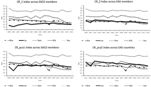
Results of the evaluation exercise for the composite indices are presented in Figure 1 below. Eswatini has the highest composite index value followed by Namibia. Lesotho and South Africa have the lowest. These results are robust to the respective aggregation and weighting procedures used.

Figure 1. Differences between risk indices constructed using different aggregation and weighting procedures.

4.2. Gravity model

The Hausman test was used to validate the use of the fixed effects model specifications. The test was marginally conclusive, with a test statistic of 18.98 (0.0042).

Table 5 below presents the results from the gravity model estimation. It shows the impact of the risk composite indices for the importer and exporter on bilateral trade volumes. The significant coefficients are presented in bold-face print with an asterisk indicating the level of significance; robust standard errors are shown in parenthesis.

Table 5. Gravity equation results using different estimators.

Model Estimators: Dependent variable:	RE (PPML) Xij	Pooled (OLS) Ln(Xij)	FE Ln(Xij)	RE (GLS) Ln(Xij)	FGLS Ln(Xij)	RE (MLE) Ln(Xij)
lnGDPj	0.627* (0.000223)	−0.124*** (0.378)	−1.94*** (1.08)	−2.01** (1.07)	−2.04*** (1.30)	−2.01* (0.825)
lnGDPi	−1.78* (0.000290)	−0.267 (0.356)	3.20** (1.52)	3.25** (1.50)	3.84* (1.39)	3.24* (0.887)
lnDistanceij	−1.54*** (0.886)	−1.91* (0.712)		−2.16** (0.100)	−2.05* (0.772)	−2.16** (0.986)
lnPopj	7.46* (0.000954)	0.512 (1.18)	−3.35 (4.05)	−3.35 (4.04)	2.72 (4.93)	3.35 (3.10)
lnPopi	4.60* (0.00102)	1.83 (1.21)	−8.49 (6.02)	−8.16 (5.97)	−7.93*** (4.84)	−8.16* (3.07)
lnRj	0.0567* (0.0000769)	0.173 (0.355)	0.701** (0.319)	−0.712** (0.319)	0.527 (0.413)	0.712* (0.258)
lnRi	−0.994* (0.0000852)	−0.440 (0.463)	−0.575 (0.411)	−0.559 (0.405)	−0.515 (0.427)	−0.559** (0.271)
Borderij	−3.33*** (1.80)	−0.729 (1.26)		−1.28 (1.85)	−0.652 (1.50)	−1.28 (1.92)
Languageij	0.212 (1.52)	2.68 (3.06)		21.8 (16.5)	18.4 (15.2)	21.8** (9.65)
Colonyij	1.96*** (1.11)	2.05* (0.95)		4.75 (3.73)	4.08 (3.16)	4.75** (2.31)
Currency	5.45* (1.53)	−1.99** (0.918)		−2.41 (2.88)	−0.927 (2.91)	2.41 (2.17)
Landlockedij	−1.91*** (3.09)	−3.07 (2.60)		−8.41 (7.40)	−6.96 (6.86)	−8.41 (5.49)
R^2		46	31	63
Prob > F	0.0000	0.0000	0.0000	0.0000	0.0000	0.0000
N	6300	2299	2299	2299	2299	2299
Log likelihood	−2.414e+09				−5658.47	−4864.4
Wald chi^2	9.35e+08		925.3	925.3	2052.1	271.5

*, **, and *** are confidence levels at the 1%, 5% and 10% respectively.

An increase in risk, generally acts as an impediment to trade as it raises the transactional costs of doing business and thus lowers the volume of international trade flows (Nitsch & Schumacher, 2004).

International trade has been identified as a possible vehicle for economic transformation in the developing world, however risk as also been flagged as an impediment to sustainable trade relations. Relying on risk-trade studies done in the developed country context will not provide the necessary answers for developing countries. There is a need for a more comprehensive approach in the developing world which will draws attention to diverse risks. This approach should also propose instruments of dealing with these diverse risks (Holzmann et al. 2003).

However in spite of its growing importance in world trade, risk has still not been fully integrated in decision making (Baas, 2010). This is partly due to the lack of a framework that quantifies and measures aggregate risk in an economy. This section presents the results from the gravity model augmented with a composite risk index. The index measures aggregate risk and Table 5.20 presents the impact of such risk on bilateral agricultural-commodity trade volume between the SACU member states.

The variables of interest are the log of risk for the importer and exporter. They are both significant indicating a substantial effect of risk on bilateral trade albeit with different signs indicating opposite effects. The coefficient of the log of risk on the importing country is 0.0567, though not overly substantial, it still means a 0.6% increase in imports for a 10% increase in risk in the domestic economy. This result was expected because an increase in risk in the domestic economy could potentially disrupt the production of goods and services by domestic producers. As such, domestic producers would be unable to meet domestic demand and therefore goods would have to be sourced from foreign producers.

The exporter risk variable on the other hand is negative and highly significant. A one percent increase in the incidence of risky events in the exporting economy would decrease bilateral trade by 1% (coefficient is −0.99). Again, this result is expected as an increase in risk in the exporting country would mean that fewer goods are produced and available for export. According to the results, aggregate risk on the importing economy leads to an increase in bilateral trade, whereas it decreases bilateral trade on the exporting end.

As expected, the distance variable is significant and negative. This means the greater the distance, the lesser will be commodity trade between the trading partners. This result implies that distance discourages bilateral trade within SACU member states. A percent increase in distance reduces commodity trade by 1.54%. This value is higher than the unity reported in the empirical literature (Anderson & van Wincoop, 2003; Martinez-Zarzoso & Nowak-Lehmann, 2003; Baier & Bergstrand, 2009).

The results show that the importer and exporter GDPs are both important factors in bilateral trade, they both have significant coefficients albeit with different signs. The sign of the importer GDP variable is positive. This means that an increase in GDP (growth in the domestic economy) increases imports as domestic consumers increase their consumption of food commodities. This is however contrary to Engel’s law, which stipulates that when dealing with agricultural commodities, the GDP of the importing country should be negative. This is because as GDP increases, the proportion spent on food commodities decreases (Foellmi & Zweimuller, 2008). However, this result is probable in the case of developing countries where the growth in GDP might not translate into an equitable distribution of real income.

The log of GDP variables which are proxies for economic size are also important determinants of bilateral trade. The coefficients for both the importer and exporter are significant with values of 0.627 and −1.78 respectively. This means a 10% increase in economic size for the importer leads to a 6.3% increase in bilateral trade. This result was expected as an increase in economic size could increase disposable income and therefore the demand for normal goods.

This increase in goods could be through the extensive margin of trade (which is the entry of new goods) or intensive margin (increased trade of existing goods in the market). This could also lead to an increase in imports to meet domestic demand. The elasticity of the importer GDP is lower than unity and has been described as evidence of home market effects (Feenstra, 2002).

However, the log of GDP variable for the exporter is negative. This means a 1% increase in economic size would lead to a 1.8% decrease in bilateral trade. An increase in disposable income in the domestic economy might increase the demand for locally produced goods and thereby decrease the amount of goods available for export.

The population variables for both the importer and exporter were also found to be important determinants of bilateral trade flows. They are both significant and they have the expected signs. A 1% increase in population leads to a 7.46% and 4.60% increase in bilateral trade for the importer and exporter, respectively. This result was expected as according to economic theory, population is one of the key determinants of demand. For the importer, an increase in population means more mouths to feed for domestic producers. The inability of domestic producers to meet this increased demand could lead to an increase in imports as foreign suppliers enter the market. On the export side, an increase in population could lead to an increase in domestic investments as producers gear up for the increased demand. This could lead to an increase in the volume of goods produced in the domestic economy and consequently the volume available for export.

All the dummy variables were also found to have an impact on bilateral trade flows in SACU except language. Currency had the largest impact on bilateral trade in absolute terms, with a coefficient of −5.45. This means that membership in the Common Monetary Agreement (CMA) where the Rand is used as a common currency leads to a 1% decrease in bilateral trade on average. This result was unexpected because according to Rose (2000), currency unions are expected to increase trade. However, it is possible that they could potentially decrease bilateral trade in the long term (De Sousa, 2012).

An interesting finding is that even after controlling for distance and membership in the trade agreement, contiguity still has an important impact on bilateral trade between SACU countries. The border dummy is significant and positive with a coefficient of 3.33. This means sharing a border increases bilateral trade by 27% on average. This is an important result as it outlines the impact of geographical distance as a source of trade costs even with trade agreements. Countries that share common colonial ties, e.g. South Africa and Namibia; The BEL countries, are expected to trade 6.1% more than countries without such ties. This is deduced from a positive and significant colony dummy variable with a coefficient of 1.96. As expected from the literature, landlocked countries are expected to trade less than countries which have excess to the sea. The coefficient for the landlocked variable is −1.91 and it is significant. Botswana, Lesotho and Eswatini as the landlocked members in the SACU bloc are expected to trade 0.85% less than South Africa and Namibia.

5. Conclusion

This paper investigated the impact of aggregate risk on bilateral trade within SACU. In the empirical analysis, the gravity model of trade was augmented with a risk index which quantified risk in the economies of the SACU member states.

Summarising the key results, the importer and exporter risk variables were found to be significant albeit with different signs. The risk variables of the importer and exporter were found to be positively and negatively correlated with bilateral trade, respectively. This means that risk increases imports and decreases exports. The exporter risk had a higher impact on bilateral trade flows than the importer risk in absolute terms. These results were robust under a number of model specifications and estimators.

Since the results reveal that risk increases imports and decreases exports between bilateral partners, it can be deduced that risk increases the dependency of the BELN countries on South Africa. There is a need for the BELN countries to increase their exports into the South African market. This will not only improve their terms of trade, but also their share from the SACU common revenue pool. This also has the potential of increasing trade volumes within the trade bloc and this would help the bloc remain relevant and sustainable.

As expected, the results show that the dominant economy in the SACU bloc, South Africa has the lowest risk in almost all the reviewed risk categories. This is not surprising as South Africa has a relatively less risky economy due to it being stable, and diversified compared to the BELN countries. This means the South African economy is more resilient, i.e. better suited to respond and recover from external shocks.

Due to their inherently low resilience, developing countries need effective strategies to deal with diverse risks. However, for this to be realist exercise in a developing country context, there is a need to be pragmatic in assessing the risks and instruments used to deal with them.

Risk needs to be addressed by improving the resilience of the domestic economy to potential crises through contingency planning. However, the starting point of the implementation of an effective and proper risk management policy is a thorough understanding of the type and dynamics of the risks involved and vulnerabilities thereof. If the BELN countries are to realise their comparative advantage in trade, SACU needs to help member countries in building their resilience through collective risk mitigation policies and strategies. This can be done by increasing the developmental component of SACU receipts and making sure it is used for its intended purpose.

Acknowledgements

The authors are indebted to Prof. C.B. Blignaut for his invaluable contribution in the early stages of the research. The authors would also like to acknowledge the African Economic Research Consortium for funding this research. The authors also appreciate the comments of the anonymous reviewers.

Disclosure statement

No potential conflict of interest was reported by the authors.

ORCID

S. S. B. Mlipha http://orcid.org/0000-0002-8300-4634

Additional information

Funding

This work was supported by African Economic Research Consortium [grant number AP13P03].

References

- Abadie, A & Gardeazabal, J, 2008. Terrorism and the world economy. European Economic Review 52, 1–27. doi: 10.1016/j.euroecorev.2007.08.005
- Aguna, CG & Kovacevic, M, 2011. Uncertainty and sensitivity analysis of the human development index. http://hdr.undp.org/sites/default/files/hdrp_2010_47.pdf. Accessed 4 October 2016.
- Anderson, JE, 2011. The gravity model. Annual Review of Economics 3, 133–60. doi: 10.1146/annurev-economics-111809-125114
- Anderson, JE & Marcouiller, D, 2002. Insecurity and the pattern of trade: An empirical investigation. Review of Economics and Statistics 84(2), 342–52. doi: 10.1162/003465302317411587
- Anderson, JE & van Wincoop, E, 2003. Gravity with gravitas: A solution to the border puzzle. American Economic Review 93(1), 170–92. doi: 10.1257/000282803321455214
- Anderson, JE & Yotov, YV, 2012. Gold standard gravity. NBER working paper. http://fmwww.bc.edu/EC-P/wp795.pdf. Accessed 6 August 2014.
- Baas, D, 2010. Approaches and challenges to political risk assessment: The view from export development Canada. Risk Management 12(2), 135–62. doi: 10.1057/rm.2009.19
- Baier, SL & Bergstrand, JH, 2009. Bonus vetus OLS: A simple method for approximating international trade-cost effects using the gravity equation. Journal of International Economics 77, 77–85. doi: 10.1016/j.jinteco.2008.10.004
- Barro, RJ, 2013. Inflation and economic growth. Annals of Economics and Finance 14(1), 85–109.
- Bayer, R & Rupert, MC, 2004. Effects of civil wars on international trade, 1950-92. Journal of Peace Research 41(6), 699–713. doi: 10.1177/0022343304047433
- Bergstrand, JH, Larch, M & Yotov, YV, 2015. Economic integration agreements, border effects, and distance elasticities in the gravity equation. European Economic Review 78, 307–27. doi: 10.1016/j.euroecorev.2015.06.003
- Bhagwati, J & Srinivasan, TN, 2002. Trade and poverty in the poor countries. American Economic Review 92(2), 180–3. doi: 10.1257/000282802320189212
- Borodin, K & Strokov, A, 2014. Inflation and the pattern of trade: General conclusions and evidence for Russia. http://ageconsearch.umn.edu/bitstream/195708/2/Borodin_Strokov_Inflation_and_the_pattern_of_trade_2014_IAMO.pdf. Accessed 29 October 2015.
- Bougheas, S, Demetriades, PO & Morgenroth, ELW, 1999. Infrastructure, transport costs and trade. Journal of International Economics 47, 169–89. doi: 10.1016/S0022-1996(98)00008-7
- De Sousa, J, 2012. The currency union effect on trade is decreasing over time. Economics Letters 117(3), 917–20. doi: 10.1016/j.econlet.2012.07.009
- Draper, P, Halleson, D & Alves, P, 2007. SACU. Regional integration and the overlap issue in Southern Africa: From spaghetti to cannelloni? The South African Institute of International Affairs. Trade Policy Report No. 15. https://www.saiia.org.za/wp-content/uploads/2008/11/SAIIA-2007-Trade-Report-No-15.pdf. Accessed 22 April 2015.
- FAO (Food and Agriculture Organization of the United Nations), 2012. Why has Africa become a net food importer? Explaining African agricultural and food trade deficits. Rome. http://www.fao.org/docrep/015/i2497e/i2497e00.pdf. Accessed 12 November 2017.
- Feenstra, RC, 2002. Border effects and the gravity equation: Consistent methods for estimation. Scottish Journal of Political Economy 49(5), 491–506. doi: 10.1111/1467-9485.00244
- Fischer, S, 1993. The role of macroeconomic factors in growth. Journal of Monetary Economics 32(3), 485–512. doi: 10.1016/0304-3932(93)90027-D
- Foellmi, R, & Zweimuller, J, 2008. Structural change, Engel's consumption cycles and Kaldor's facts of economic growth. Journal of Monetary Economics 55(7), 1317–28. doi: 10.1016/j.jmoneco.2008.09.001
- Fosu, AK, 2001. Political instability and economic growth in developing economies: some specification empirics. Economics Letters 70, 289–94. doi: 10.1016/S0165-1765(00)00357-8
- Goldberg, PK & Pavcnik, N, 2004. Trade, inequality, and poverty: What do we know? Evidence from recent trade liberalization episodes in developing countries. NBER working paper no. 10593. http://www.eldis.org/document/A16033. Accessed 4 July 2018.
- Hagerty, MR & Land, KC, 2007. Constructing summary indices of quality of life: A model for the effect of heterogeneous importance weights. Sociological Methods and Research 35(4), 455–96. doi: 10.1177/0049124106292354
- Hair, JF, Black, WC, Babin, BJ & Anderson, RE, 2010. Multivariate data analysis. 7th edn. Pearson Prentice Hall, Upper Saddle River, NJ.
- Head, K & Mayer, T, 2013. Gravity equations: Workhorse, toolkit, and cookbook. Centre for Economic Policy Research. Discussion Paper No: 9322. http://strategy.sauder.ubc.ca/head/papers/headmayer_revised.pdf. Accessed 6 June 2014.
- Holzmann, R, Sherburne-Benz, L & Tesliuc, L, 2003. Social risk management: The World Bank’s approach to social protection in a globalizing world. http://siteresources.worldbank.org/SOCIALPROTECTION/Publications/20847129/SRMWBApproachtoSP.pdf. Accessed 12 September 2015.
- IMF (International Monetary Fund), 2014. Regional economic outlook. Sub-Saharan Africa. https://www.imf.org/external/pubs/ft/reo/2014/afr/eng/sreo1014.pdf. Accessed 6 June 2016.
- Keshk, OMG, Reuveny, R & Pollins, BM, 2010. Trade and conflict: Proximity, country size, and measures. Conflict Management and Peace Science 27(1), 3–27. doi: 10.1177/0265659009352137
- Kirk, R & Stern, M, 2005. The new Southern African Customs Union agreement. The World Economy 28(2), 169–90. doi: 10.1111/j.1467-9701.2005.00619.x
- Limao, N & Venables, A, 2001. Infrastructure, geographical disadvantage, transport costs, and trade. The World Bank Economic Review 15(3), 451–79. doi: 10.1093/wber/15.3.451
- Long, AG, 2008. Bilateral trade in the shadow of armed conflict. International Studies Quarterly 52, 81–101. doi: 10.1111/j.1468-2478.2007.00492.x
- Martin, W & Pham, CS, 2008. Estimating the gravity model when zero trade flows are frequent. Economics series; MPRA paper no. 9453. https://ideas.repec.org/p/dkn/econwp/eco_2008_03.html. Accessed 23 February 2016.
- Martinez-Zarzoso, I, Felicitas, NLD & Horsewood, D, 2009. Are regional trading agreements beneficial? Static and dynamic panel gravity models. The North American Journal of Economics and Finance 20, 46–65. doi: 10.1016/j.najef.2008.10.001
- Martinez-Zarzoso, I & Nowak-Lehmann, F, 2003. Augmented gravity model: An empirical application to MERCOSUR-European Union trade flows. Journal of Applied Economics 6(2), 291–316. doi: 10.1080/15140326.2003.12040596
- Mirza, D & Verdier, T, 2008. International trade, security and transnational terrorism: Theory and a survey of empirics. Journal of Comparative Economics 36, 179–94. doi: 10.1016/j.jce.2007.11.005
- Nardo, M, Saisana, M, Saltelli, A & Tarantola, S, 2005. Tools for composite indicators building. European Commission. http://citeseerx.ist.psu.edu/viewdoc/download?doi=10.1.1.114.4806&rep=rep1&type=pdf. Accessed 19 May 2016.
- Ndulu, B, Kritzinger-van Niekerk, L & Reinikka, R, 2005. Infrastructure, regional integration and growth in Sub-Saharan Africa: in Africa in the world economy. http://www.fondad.org/product_books/pdf_download/5/Fondad-AfricaWorld-BookComplete.pdf. Accessed 23 April 2014.
- Ngalawa, HPE, 2013. Anatomy of the Southern African Customs Union: Structure and revenue volatility. ERSA working paper 374. http://www.econrsa.org/system/files/publications/working_papers/working_paper_374.pdf. Accessed 10 September 2014.
- Nicoletti, G, Scarpetta, S & Boylaud, O, 2000. Summary indicators of product market regulation with an extension to employment protection legislation. OECD. Economics Department working paper no. 226, OECD. http://dx.doi.org/10.1787/215182844604. Accessed 26/04/2016.
- Nitsch, V & Schumacher, D, 2004. Terrorism and international trade: An empirical investigation. European Journal of Political Economy 20, 423–33. doi: 10.1016/j.ejpoleco.2003.12.009
- OECD (Organisation for Economic Co-operation and Development), 2008. Handbook on constructing composite indicators. Methodology and user guide. OECD Publishing. Paris. https://www.oecd.org/std/42495745.pdf. Accessed 22 March 2016.
- Oh, CH & Reuveny, R, 2010. Climatic natural disasters, political risk, and international trade. Global Environmental Change 20, 243–54. doi: 10.1016/j.gloenvcha.2009.11.005
- Prehn, S, Brummer, B & Glauben, T, 2016. Gravity model estimation: Fixed effects vs. random intercept Poisson pseudo-maximum likelihood. Applied Economics Letters 23(11), 761–4. doi: 10.1080/13504851.2015.1105916
- Raddatz, C, 2007. Are external shocks responsible for the instability of output in low-income countries? Journal of Development Economics 84, 155–87. doi: 10.1016/j.jdeveco.2006.11.001
- Rose, AK, 2000. One money, one market: Estimating the effect of common currencies on trade. Economic Policy 30, 9–45.
- SACU (South African Customs Union), 2014. Publications. SACU agreements. http://www.sacu.int/main.php?include=docs/legislation/1910-agreement.html. Accessed 29 April 2014.
- Saisana, M, Saltelli, A & Tarantola, S, 2005. Uncertainty and sensitivity analysis techniques as tools for the quality assessment of composite indicators. Journal of the Royal Statistical Society: Series A (Statistics in Society) 168(2), 307–23. doi: 10.1111/j.1467-985X.2005.00350.x
- Salvatici, L, 2013. The gravity model in international trade. AGRODEP technical note TN-04. http://www.agrodep.org/sites/default/files/Technical_notes/AGRODEP-TN-04-2_1.pdf. Accessed 12 August 2014.
- Santos Silva, JMC & Tenreyro, S, 2006. The log of gravity. Review of Economics and Statistics 88(4), 641–58. doi: 10.1162/rest.88.4.641
- Susanto, D, Rosson, CP & Costa, R, 2010. Financial development and international trade: Regional and sectoral analysis. https://core.ac.uk/download/pdf/6833591.pdf. Accessed 29 October 2015.
- Tansey, MM & Touray, A, 2010. The gravity model of trade applied to Africa. International Business & Economics Research Journal 9(3), 127–30.
- Tate, E, 2012. Social vulnerability indices: A comparative assessment using uncertainty and sensitivity analysis. Natural Hazards 63(2), 325–47. doi: 10.1007/s11069-012-0152-2
- WEF (World Economic Forum), 2013. Global risks 2013. http://www3.weforum.org/docs/WEF_GlobalRisks_Report_2013.pdf. Accessed 24 September 2014.
- Westerlund, J & Wilhelmsson, F, 2011. Estimating the gravity model without gravity using panel data. Applied Economics 43, 641–9. doi: 10.1080/00036840802599784