Optimising balance using covariate balancing propensity score: The case of South African child support grant

ABSTRACT

In this paper, we explore the use of covariate balancing propensity scores (CBPS) in estimating the impact of the South African child support grant (CSG) on the height-for-age score of benefiting children. CBPS is a different approach to estimating propensity score, under CBPS the scores are estimated such that the estimation incorporates covariate balancing condition. This approach is therefore relatively robust to misspecification of the propensity score model which makes it ideal for this case study. We show that utilising the CBPS leads to treatment effect estimate that is larger and more precisely estimated than estimates that have been reported in the literature because the method exploits the dual function of propensity score. The effect of CSG under CBPS is as large as 44% of standard deviation on average. This implies that the effect of the grant cannot be regarded as small as previously reported in the literature.

KEYWORDS:

• Covariate balancing propensity score
• stunting
• height-for-age score
• malnutrition

JEL:

• I38
• H53
• D13

1. Introduction

Nutrition is important for the growth of children. Malnutrition, especially during the early stages of life, cannot only be detrimental to the general well-being of affected children, research also suggests that it may also contribute to intergenerational transmission of poverty (Delany et al., 2008; Walker et al., 2015). Children born to stunted parents are more likely to have a low score on the cognitive scale, have lower development quotient and are likely to be stunted themselves (Walker et al., 2015).

The South African child support grant (CSG) is one of the social assistance programmes that was designed to address the inequality in South African society. This social transfer is intended to mitigate the effect of poverty and inequality on vulnerable children in poor households. It is, therefore, logical to expect that poor families will utilise this grant to improve the wellbeing of benefiting children. Statistics South Africa reports that poor households spend about a third of their income on food.¹ Therefore one should expect that the CSG will have an effect on the variable that captures the cumulative effects of malnutrition in benefiting children relative to eligible non-benefiting children.

This paper examines the effect of the CSG on the height-for-age of benefiting children. We assume that poor households that benefit from the CSG will use it to purchase food items (amongst other things) to improve the well-being of children. Under the assumption that the food items are well utilised by benefiting children, one should expect the CSG to have a positive significant effect on the height-for-age of benefiting children.

Existing literature suggests that the effect of the CSG on height-for-age of benefiting children is generally small especially in the binary treatment case. For example, in the binary treatment case, Coetzee (2011) and Aguero et al. (2006) found that CSG has no significant effect on height-for-age.² Heinrich et al. (2012) found an effect only for girls whose mothers have eight or more grades of schooling (19% of standard deviation). In the continuous treatment case Aguero et al. (2006) and Coetzee (2013) reported maximum effect of 25% and 4% of standard deviation³ respectively. In this paper, we show that a more meaningful estimate of the CSG can be recovered from the NIDS wave 1 data (without compromising on balance). We also show that using the covariate balancing propensity score (CBPS) method to improve on the existing method (by this we mean the logit Propensity score matching), the effect of CSG on the height-for-age score is larger than previously reported in the literature. Our result shows that the effect of CSG on height-for-age is up to 44% of a standard deviation on average (i.e. in the binary treatment case). In terms of method we provide an explanation as to why the proposed CBPS performs better in this case study.

The rest of the paper is organised as follows section 2 provides some clarifications and justification for the study and section 3 present a brief review of the data. In section 4, we discuss the CBPS technique and the changes made to the estimation process. Section 5 presents the results while section 6 explores the reason why the effect estimate under CBPS is different from the one estimated under the conventional logit model. Section 7 concludes.

2. Literature review and justification for the study

2.1. Brief review on the South African CSG

The CSG is an unconditional grant intended to assist poor households in improving the welfare of children in such households. While there are soft conditions related to school attendance attached to the grant, failure to comply is not exclusionary (Oyenubi, 2018). Therefore, the CSG gives the caregivers full autonomy on how the grant is spent. This makes evaluating the impact of the grant more complicated as against conditional grants whose direct response are prescribed by the conditions attached to the grant. The Child Support Grant (CSG) was introduced in 1998 and has since undergone administrative and several policy changes to redefine eligibility over the years (d’Agostino et al., 2017). In general, eligibility is based on means test (this will be discussed further in section 3).

A number of studies have explored the impact of the CSG on a range of outcome variables. These variables include education, health, and nutrition. Case et al. (2005) using data from the KwaZulu-Natal Income Dynamics Study finds that the CSG improves the probability of school enrolment amongst benefiting children. Aguero et al. (2006), using the same dataset and under the assumption that treatment effect is continuous, finds that high dosage of the CSG early in life has a positive impact on child nutrition. Coetzee (2013) investigates the impact of the CSG on a range of outcome variables that includes height-for-age score, food expenditure, adult expenditure and progress through school. The author makes use of Wave 1 of the National Income Dynamics Study (NIDS). Like Aguero et al. (2006), Coetzee (2013) finds positive, albeit small, effect on three of the selected outcomes⁴ under the assumption that the treatment is continuous.

2.2. Review on the CBPS

Aguero et al. (2006; footnote 15) and Coetzee (2011: 2) (the working paper version of Coetzee (2013)) noted that using Propensity Score Matching (PSM), no significant treatment effect was found for the outcome variables considered in both studies. Furthermore, in the appendix of Coetzee (2011), section 3 noted that the inclusion of a variable that capture caregiver’s eagerness⁵ to apply for the programme resulted in a situation where a propensity score specification that balances the distribution of covariates was not found (using the algorithm of Dehejia & Wahba (1999, 2002)⁶). Coetzee (2011) therefore excluded this variable in the subsequent analysis.

We note that implementation problems associated with the PSM approach are well known and documented in the literature (see Diamond & Sekhon (2013), Imai & Ratkovic (2014) and Hainmueller (2012, 2013)). PSM seeks to balance the propensity score density, however, balance in the propensity score density may not translate into balance in the other covariates. Furthermore, lack of balance in relevant covariates after matching on estimated propensity scores may signal misspecification of the propensity score equation (Caliendo & Kopeinig, 2008). Since the true propensity score is unknown and has to be estimated, an iterative search over propensity score models is conducted to find the appropriate specification. This manual optimisation of balance is often tedious in practice and is not guaranteed to yield satisfactory results.

However, maintaining the assumptions that validate propensity score matching (PSM), i.e. selection on observables and common support assumption alternative ways of estimating propensity score and balancing weights has been introduced in the literature. These methods side-line the specification search by focusing directly on balance in the relevant covariates (e.g. Diamond & Sekhon (2013)) or estimating propensity scores that incorporate the balancing condition (Imai & Ratkovic, 2014). In this study, we use the method introduced by Imai & Ratkovic (2014) to address the problems noted by Aguero et al. (2006) and Coetzee (2011). The CBPS estimate propensity scores that incorporate the balancing condition. Specifically, the regular propensity score involves optimising a likelihood function to estimate the probability of treatment. CBPS optimises the likelihood function under the constraint that the balancing condition is satisfied.

The CBPS approach represent a significant improvement on the PSM method for a number of reasons. First, this method avoids the iterative model specification search and balancing assessment that is often necessary under conventional propensity score methods. Second, CBPS achieves this by exploiting the dual characteristics of the propensity score as a balancing score and the conditional probability of treatment assignment. Lastly, CBPS has been shown to perform better than PSM in terms of bias and Mean Square Error (MSE) in a simulation study (Imai & Ratkovic, 2014).

2.3. Possibility of catch-up growth

The consensus in the literature is that height-for-age can serve as an ex-post indicator of nutritional imputes, stunting or low height-for-age (<−2) is an indicator of long-term malnutrition. The literature also suggests that nutritional deficiencies in the first 3 years of life may not be reversible (Heinrich et al., 2012; Duflo, 2003), i.e. nutritional deficiencies that manifest as low height-for-age score may leave a permanent mark on the height-for-age score of children. However, a strand of the literature suggests that under the right conditions malnourished children can experience catch-up growth. Catch-up growth is defined as rapid linear growth that allows the child to accelerate toward and, in favourable circumstances, resume his/her pre-illness growth curve (Boersma & Wit, 1997). This suggests that even if children are malnourished in the first 3 years of life, CSG receipt can help them recover some of the lost grounds relative to eligible non-benefiting children. Although we note that Desmond & Casale (2017) provide evidence that while the catch-up growth is possible stunted children at age 2 may not fully recover in terms of cognitive ability.

Therefore following Coetzee (2013, 2011), our sample is made up of children that are 14 years old or younger. We note that although it may be optimal to assess that effect of the CSG on height-for-age scores during the first 3 years of life, this does not rule out the possibility of a positive improvement in growth outside the 3-year window (Aguero et al., 2006).

2.4. Continuous versus binary treatment and effect size

It has been argued in the literature (see Aguero et al. (2006) and Coetzee (2013)) that the effect of CSG should ideally be modelled as continuous treatment, this allows the cumulative effect of the income flows to be accounted for. However, this does not preclude the argument that if there is a significant effect in the continuous treatment case, there could be some effect in the binary treatment case (i.e. when treatment is modelled as a binary variable) albeit this will represent the lower bound of the treatment effect. Furthermore, dosage (or duration of benefit) can be controlled for in the binary treatment case (Oyenubi, 2018).

We note that the continuous treatment framework fails in part to answer a question that may be argued to be of importance from the policy perspective. This is because, by definition, continuous treatment under the generalised propensity score (GPS) approach considers only treated units and measures the effect of different levels of treatment (treatment dosage). In other words, the ‘control group’ in this framework consists of children with a lower treatment dosage as against eligible non-benefiting children. While it is useful to know that increased dosage has a positive effect on the height-for-age score (Coetzee, 2013), the comparison between eligible beneficiaries and eligible non-beneficiaries remains an important question of interest in our opinion. This answers the question as to whether it is optimal to opt into the programme in the first place. Although one can infer that if a higher dosage has a positive effect on the height-for-age score of benefiting children, these children should be doing better than (comparable) eligible non-beneficiaries with respect to height-for-age. This will, however, be an assumption and this assumption will not give an indication of the size of the effect of the policy.

Continuous versus binary treatment aside, estimates of the effect of CSG on height-for-age of benefiting children in South Africa is generally low (as noted earlier). Coetzee (2013) notes that the weak effect provides inconclusive evidence that the grant is used in improving the lives of benefiting children. By exploring the CBPS approach we examine if the weak effect is an artefact of the weakness of the PSM method as against the absence of a meaningful effect in the binary treatment case.

3. Data

This study makes use of NIDS wave 1 dataset (similar to Coetzee (2011, 2013)). This allows us to compare our results with the estimate in Coetzee (2011). The wave 1 survey was conducted in 2008. Eligibility for CSG is determined by the age and means tests that were in effect in 2008.⁷ We use the age and means test to identify treated children. A child is assigned to the treatment group if it is indicated that CSG is currently being received for the child or another child that resides in the household.

This is because the definition of households in NIDS require that members of a household share food from a common source. Control group consist of children who live in households that are eligible (i.e. have a child or children that are eligible) for the grant but are not receiving the grant.

We restrict the sample to the population of black children since blacks are the majority in South Africa and genetic factors can influence the height-for-age of children across race groups.⁸ Table 1 shows the summary statistics for the data. Table 1 shows that caregivers of treated children delay for 3.5 years on average while control group caregivers delay for 9.8 years on average. As a consequence, estimated motivation is lower in the control group compared to the treatment group (we discuss the construction of the motivation variable in the next section). Control group caregivers are more likely to be married, more likely to be employed, less educated and older when compared to treated group caregivers. Control group children are older, less likely to live in rural areas and less likely to be living with their father or mother.

Table 1. Summary statistics.

Variable	Mean	SD	Mean	SD	Mean	SD
	All (3451)		Treated(2415)		Control(1036)
w1_zhfa	−0.98	1.49	−0.96	1.51	−1.02	1.44
Delay(yrs)	5.08	4.6	3.46	3.34	8.84	4.92
motivation	0.03	1.01	0.44	0.88	−0.92	0.57
employed	0.25	0.44	0.25	0.43	0.26	0.44
married	0.37	0.48	0.35	0.48	0.42	0.49
PC edu	6.57	4.59	6.97	4.5	5.64	4.67
PC age	41.53	15.59	39.62	14.33	45.97	17.41
Hh head gen	0.36	0.48	0.37	0.48	0.35	0.48
Child gender	0.5	0.5	0.5	0.5	0.51	0.5
electricity	0.63	0.48	0.62	0.49	0.64	0.48
water	0.17	0.37	0.16	0.36	0.19	0.4
telephone	0.03	0.17	0.03	0.17	0.03	0.18
toilet	0.2	0.4	0.19	0.39	0.23	0.42
Ae food expenditure	187.92	125.64	184.33	115.03	196.29	147.15
Informal dwelling	0.07	0.25	0.07	0.26	0.06	0.24
Child age	7.89	4.27	7.4	3.87	9.04	4.88
rural	0.75	0.43	0.76	0.43	0.72	0.45
PC relationship	0.64	0.48	0.71	0.45	0.47	0.5
low birthweight	0.03	0.16	0.03	0.18	0.01	0.12

*PC edu Primary Caregiver education (years); PC Age Primary Caregiver’s age (yrs); HH head gen Gender of head of household; Ae food expenditure Adult equivalent food expenditure; PC relationship Child’s relationship with primary caregiver

4. Method

Apart from the use of CBPS, this paper makes a number of changes to the sample used by Coetzee (2011, 2013). Coetzee’s sample included only children that are born 2 years or more prior to the NIDS survey. The author argues that average delay in taking up of CSG stabilises after 2 years from birth (also see Aguero et al. (2006)) so that average delay (before receiving the grant) for children under 2 years will be underestimated. However, excluding this cohort of children is problematic since this period falls within the critical period where deficiencies in height-for-age are critical to the development of the child going forward. Furthermore, excluding this cohort of children may not be ideal for the binary treatment case, therefore we include children in this age cohort in our analysis.

4.1. Calculating the motivation variable

Existing literature suggests that unobserved variation in caregivers eagerness to apply for the grant may bias the treatment effect (Aguero et al. (2006); Coetzee (2011, 2013)). To proxy for this variable, a variable that captures unobserved differences in caregiver’s eagerness or motivation to apply for the grant is derived from the data. This is important because caregivers with higher motivation will apply for the CSG earlier than those with lower motivation and this will affect the treatment effect through the dosage of treatment. Therefore children with a motivated caregiver will receive higher dosage and therefore will benefit more relative to children with a less motivated caregiver.

To derive this variable, the delay before applying for the grant is assumed to be a function of the effectiveness of the roll-out of the CSG in the area where the child lives and the age of the child. Caregiver motivation is then calculated by standardising the difference between actual delay and expected delay.

Calculation of actual delay depends on the child’s treatment assignment. For example in Coetzee (2011), actual delay for treated children is the difference between the child’s birthday and the day CSG was first received for the child. For control group children, actual delay is calculated as the difference between the child’s birthday and the date the child was interviewed Coetzee (2011: 9). Expected delay is then calculated as the Ordinary least squares (OLS) prediction of delay given the child’s age and location (rural or urban).

By construction, the approach just discussed guarantees that there will be an imbalance in the data since the motivation variable has to be different across the treatment and control groups. Especially because interview date is used for children in the control group. This does not necessarily imply that respondents in the two groups are very different. This is more likely the consequence of not accounting for the fact that a delay in the control group may not be equal to the child’s age. That is, some caregivers in the control sample may have applied for CSG and not received it (Oyenubi, 2018).

Actual delay for the treated children in this paper follows the approach used in Coetzee (2013), however, to calculate expected delay for the control group, we follow the approach in (Oyenubi, 2018). To calculate delay for the control group we use the information on whether the caregiver has ever applied for CSG on behalf of the child. The reason is that the caregivers that have made an effort to apply for the grant but did not succeed for whatever reason cannot be categorised as being unmotivated (in this context). However, this reduces the sample size in the control group considerably since the variable that captures the date of application for control group children has just a handful of responses. To accommodate other eligible children for whom an application has not been made we use censored regression. Control observations with no application date data are regarded as being right-censored with a variable censoring point that is equal to the age of the child (this is because an application has not been made for these children but may be made sometime in the future). The logic here is that although we did not observe delay for some control group members, we can estimate expected delay for this group by exploiting the covariates that predict delay in the data.

Lastly, our specification of the motivation equation includes a variable that was not included in Coetzee (2013). In addition to the child’s age and location (rural/urban), we control for the relationship between the child and the primary caregiver. The relationship is modelled as a binary variable that is equal to one if the primary caregiver is the father or mother of the child and zero otherwise. We include this variable because this step of the estimation process is about predicting delay. Any variable that explains significant variation in delay (in the presence of other variables) and has a reasonable justification for its inclusion should be included in the model. In our case, the argument is that there may be differences in delay that is explained by the relationship between the primary caregiver and the child. Table 2 shows that when a child’s primary caregiver is the father or mother, the delay is reduced significantly. This suggests that parents may have a higher motivation to go through the bureaucratic process of applying for CSG on behalf of their children than any other relative. The fact that this variable explains significant variation in delay in the presence of other variables justifies its inclusion as a good predictor of delay. Expected delay is then obtained as a prediction from the censored regression model.

Table 2. Censored regression to predict caregiver motivation.

Variables	(1)
	Delay in years
Child age	0.877***
	(0.019)
rural	−0.820***
	(0.164)
Caregiver relationship	−1.662***
	(0.170)
Constant	0.740***
	(0.242)
Observations	3,451

Standard errors in parentheses ***p < 0.01.

Aguero et al. (2006) and Coetzee (2011, 2013) argue that failure to control for the unobserved motivation will bias the treatment effect estimate because in the continuous treatment case dosage matters. Coetzee (2011) noted that excluding the motivation variable will violate the conditional independence assumption in the binary treatment case.⁹ If we make the reasonable assumption that the effect of CSG is heterogeneous, neglecting variation due to motivation will also bias the estimate in the binary treatment case. This is because estimated delay varies in both groups. Motivation is a function of the child’s age, relationship to caregiver and roll-out of the programme in the location where the child lives. Variation due to these factors is not peculiar to the treatment group. Therefore, the prediction from the censored regression gives us the expected delay given these covariates. Ignoring this variation (in the control group) will mean that the treatment effect may actually be the effect of how these factors interact with delay and not purely the effect of the CSG.

Our estimation still relies on the usual conditional independence and common support assumption. Following Aguero et al. (2006) and Coetzee (2011, 2013), we assume that controlling for the covariates in Table 1 addresses selection between treated and untreated children. In other words, after controlling for the measured covariates and the estimated motivation variable assignment into the two treated arms is as good as random. The main difference between our analysis and the analysis in existing studies is the way we have calculated the motivation variable and how propensity score is estimated.

4.2. Covariate balancing propensity scores

CBPS estimates the conditional probability of treatment while incorporation the balancing condition required to validate the conditional independence assumption. The problem with the existing methodology is that it focuses on estimating the conditional probability of treatment under the assumption that ‘correctly’ estimated propensity score will balance the distribution of covariates when it is used in matching or weighting estimators. However, the literature has shown that when the propensity score is slightly miss-specified it may not result in adequate balance in the distribution of covariates and as a consequence lead to substantial bias in the estimated treatment effect (Smith & Todd, 2005).

In practice, estimating propensity score involves a specification search, the estimated propensity score is appropriate only if it balances the distribution of covariates. Therefore the search involves iteratively estimating different propensity score specifications and checking for balance in the resulting matched or weighted sample until the balancing condition is satisfied.

Conventional propensity score estimation predicts the treatment assignment probability by optimising the logit (or probit) likelihood function but it ignores the other function of propensity scores, i.e. balancing the distribution of covariates. CBPS, on the other hand, trades off some treatment assignment prediction accuracy to ensure that the distribution of covariates is balanced. This means that CBPS automatically balances the distribution of the covariates. In a nutshell, one can think of the conventional logit estimation of propensity score as an unconstrained optimisation while CBPS is a constrained optimisation where the constraint is the balancing condition.

We refrain from repeating the technical details of the implementation of CBPS and refer interested readers to Imai & Ratkovic (2014) for details of the implementation of this method.

5. Results

Similar to Coetzee (2011) and Aguero et al. (2006) we assume that since benefiting household are poor households this cash injection will boost there ability to purchase more food. This is a reasonable assumption since poor households spend about a third of their income on food. Based on this we expect that the cash injection will result in improved nutrition for the benefiting children which will in turn reflect in their height-for-age scores.

To estimate the treatment effect of CSG on height-for-age of benefiting children we use both propensity score and CBPS. Our main result is based on the CBPS approach but we present result using conventional logit estimation of the propensity score to shed some light on the difference between the two approaches.

Imai & Ratkovic (2014) show that CBPS dramatically improves the poor empirical performance of propensity score matching and weighting methods. Given the observation in Coetzee (2011) about the difficulty of finding a specification that balances the distribution of covariates when the propensity score model includes the motivation variable, we note that the CBPS approach is a viable option under such condition. Similar to Coetzee (2011) we did not find a specification that balances the distribution of covariates according to the DW (Dehejia & Wahba, 1999) algorithm. Therefore, we specify the propensity score equation as a linear function of the covariates (i.e. without higher-order or interaction terms) under the conventional logit estimation and the CBPS model. We use the same specification under the two models to allow for comparison between the two methods for estimating propensity scores. For our main result, we rely on the fact that CBPS is relatively robust to misspecification of the propensity score equation. The variables we use to estimate the CBPS and the conventional logit propensity scores include motivation (which is a function of child’s age, location and relationship to the primary caregiver), caregivers employment status, marital status, age and years of education. We also control for household characteristics which include the gender of the head of household, access to electricity, water, telephone and toilet, adult-equivalent food expenditure and a dummy for informal dwelling. Lastly, we control for child characteristics, i.e. gender of the child and a dummy that indicates whether the child was born with low birth weight (Oyenubi, 2019).

5.1. Balance diagnostics CBPS versus logit propensity scores

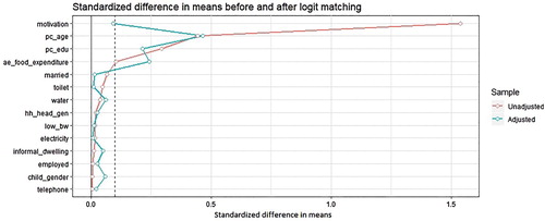
Since the DW algorithm does not work as a yardstick for balance assessment in this context, we rely on the standardised difference in means. We set a threshold of 0.1 as recommended in the literature (Austin, 2009). In other words, the imbalance is too high if the absolute difference in the means of a covariate across treatment arms is more than 1% in units of pooled standard deviation. Unlike t-tests, this measure is not influenced by sample size.

Figure 1 shows the standardised difference in means for the raw or unadjusted sample (red line) and weighted or adjusted sample (blue line) when the weights are calculated using CBPS.¹⁰ Note that the variables are arranged in the order of magnitude of the standardised difference in means in the unadjusted sample. Furthermore, note that the imbalance in the motivation variable confirms the finding of Coetzee (2011), i.e. this variable displays the highest imbalance because it is a strong predictor of treatment by construction.

Figure 1. Standardised difference in means before and after weighing under CBPS.

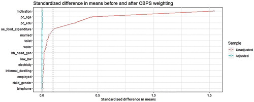
However, it is clear that using the CBPS weights removes the imbalance in the unadjusted sample as shown by the reduction in the standardised difference in means. For all covariates, the standardised difference in means for the weighted sample is below the threshold of 0.1 (dash line in Figure 1). Figure 2 presents a similar result for the conventional logit propensity score and it is also clear that for some of the covariates weighting with the odds ratio does reduce the imbalance. However, for the variables with the four largest imbalance in the unadjusted sample the reduction in imbalance did not produce a standardised difference that is below the threshold. For other variables imbalance actually increased in some cases. This is not surprising since we already know that the logit specification used may be miss-specified.

Figure 2. Standardised difference in means before and after weighing under conventional propensity score.

The implication of these results is that we cannot rely on the effect estimate that is based on the conventional logit model in this case study. We note that perhaps if one searches through all the possible combination of higher-order and interaction terms of the covariates one may be able to find a model that balances the covariates. However, the point here is that one can achieve a reasonable balance in a robust way by using CBPS.

5.2. Treatment effect estimate

To estimate the treatment effect we use weighted least squares (WLS) while controlling for other covariates for efficiency (Imai & Ratkovic (2014) also use this estimator in their simulations). We also check the robustness of the result by using robust standard errors. Table 3 presents the results for the CBPS weighting and conventional logit propensity score weighting.

Table 3. Treatment effect estimate with matching and balancing weights.

	WLS with balancing weights		WLS with Matching weights
	CBPS	PS	CBPS	PS
treatment	0.397	0.186	0.444	0.295
standard error	(0.049)***	(0.057)***	(0.083)***	(0.089)***
robust standard error	(0.165)**	(0.1472)	(0.2050)***	(0.1663)*
other covariates	yes	yes	yes	yes

Standard errors in parentheses ***p < 0.01, **p < 0.05, *p < 0.1.

The first two columns present the result from WLS regression where the weights are 1 for treated observations and the odds ratio for control observations. In the last two columns, we match using the CBPS and logit propensity scores (PS) and then use the matching weights in another WLS estimation.

The size of the treatment effects that are based on the conventional propensity scores is generally lower than the results that are based on the CBPS. One of the differences between this (matching) result and the one presented in Coetzee (2011) is that this result controls for the motivation variable (another difference is that WLS is used in this analysis). The treatment effect reported by Coetzee (2011) is 7% and it is not statistically significant, this result suggests that the size of the effect could have been larger (up to 29%, i.e. under the matching weights).¹¹

However, we note that Figures 1 and 2 suggests that we should place more weight on the CBPS results since the CBPS balances the distribution of covariates and the conventional propensity score does not. Note that this pattern is replicated when after matching balance is examined. Figures A1 and A2 (in the appendix) present balance statistics similar to Figures 1 and 2 for the unadjusted and matched data. This means the estimates based on conventional propensity scores might be biased.

The result under CBPS suggests that the treatment effect is larger and significant, i.e. 39% and 44% of standard deviation for the balancing and matching weights respectively. The size of the effect suggests that the CSG has a meaningful impact on the height-for-age score of benefiting children. The third row in Table 3 shows that the effect is significant even under robust standard error.

6. Exploring the difference between CBPS and logit propensity scores

We have noted earlier that one can view CBPS as a method that optimises the likelihood function (for prediction of the probability of treatment) with constraints that stipulate balance in the covariates. On the other hand, the conventional propensity score optimises the likelihood function alone and ignores balance in the covariates under the assumption that ‘correctly’ estimated propensity score should balance the covariates. This fails in most instances because the propensity score is not known and has to be estimated.

Since the constrained and unconstrained optimisation should produce different results we should expect the beta estimates in both models to be different. Table 4 presents the models.

Table 4. CBPS model and conventional logit model.

	CBPS		PS
	Estimate	Std. Error	Estimate	Std. Error
(Intercept)	4.88	0.478***	3.913	0.287***
motivation	2.02	0.134***	3.254	0.125***
employed	0.586	0.147***	−0.025	0.129
married	−0.234	0.126*	−0.025	0.135
pc_edu	−0.0148	0.12	−0.007	0.016
pc_age	−0.0657	0.112	−0.037	0.004***
hh_head_gen	0.0592	0.107	0.248	0.133*
child_gender	−0.602	0.122***	−0.118	0.11
electricity	−0.567	0.153***	−0.166	0.122
water	−0.229	0.131*	−0.171	0.174
telephone	1.34	0.0941***	−0.054	0.319
toilet	−0.667	0.0978***	−0.554	0.166***
ae_food_expenditure	0.000527	0.132	−0.0004	0.0004
informal_dwelling	1.07	0.138***	0.324	0.214
low_bw	1.01	0.142***	0.044	0.355

***p < 0.01, *p < 0.1.

It is clear that the relative size of covariate betas and their significance varies across the models. If we take the absolute value of the betas in each model as the influence of the variable in predicting the propensity score and we normalise the betas so that under each model the absolute values sum up to 1. This exercise gives us the relative influence (i.e. $\left|{\text{β}}_i\right|/\sum \left|{\text{β}}_i\right|$) of each variable on the scores in the two models. Table 5 presents the relative strength of each variable in each model. Note that variation in the motivation variable accounts for about 36% of the variation in the predicted propensity scores under the conventional logit model while is accounts for only 15% of the variation under CBPS (Note that apart from the intercept this variable is the most influential variable in determining variation in both variant of the propensity scores).

Table 5. Covariate influence under CBPS and logit model.

	CBPS	PS
(Intercept)	0.365674	0.437676
motivation	0.151365	0.363966
employed	0.043911	0.002796
married	0.017534	0.002796
pc_edu	0.001109	0.000783
pc_age	0.004923	0.004139
hh_head_gen	0.004436	0.027739
child_gender	0.04511	0.013199
electricity	0.042487	0.018567
water	0.01716	0.019127
telephone	0.10041	0.00604
toilet	0.04998	0.061966
ae_food_expenditure	3.95E−05	4.47E−05
informal_dwelling	0.080178	0.03624
low_bw	0.075682	0.004921

On the other hand variation in the low birthweight (low_bw) indicator is about 15 times (0.0757/0.0049) more important under the CBPS model relative to the conventional propensity score model. The point here is that since these weights (or betas) represent the influence of each variable under the two models, differences in weights should lead to differences in the shape of the propensity scores across the two models. Furthermore, balance is problematic for the conventional logit model because the motivation variable is a strong predictor of treatment and this results in common support / balance problems (Coetzee, 2011). However, in the case of CBPS, the influence of the motivation variable is reduced considerably because of balance consideration. This facilitates balance under this method relative to the conventional logit model. In other words, by reducing the influence of a variable that is a strong predictor of treatment CBPS achieves a reasonable level of balance. This reduced influence is the effect of the balance constraint.

Note that this is related to the point made by Bhattacharya & Vogt (2007), a variable that is a strong predictor of treatment may qualify as an instrumental variable. Including such variables in propensity score estimation leads to inconsistent results because of the predictive power of the instrument. Even though, in theory, not controlling for this variable may result in bias (Coetzee, 2011), controlling for it is also problematic because of its strong correlation with the treatment. CBPS trades-off treatment predictive power for balance to generate a better estimate.

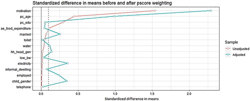
Figures 3 and 4 present the distribution of propensity scores before and after matching on CBPS and the conventional propensity scores respectively.

Figure 3. Propensity score density before and after CBPS matching.

Figure 4. Propensity score density before and after conventional propensity score matching.

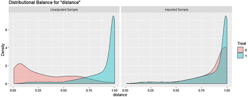
Visual inspection does suggest that density overlap in the CBPS is higher than the density overlap in the conventional propensity scores.¹² This becomes clearer when one considers the entropic distance between the unadjusted propensity scores under the two models. The entropic distance is a metric that measures the ‘distance’ between two distributions. It is given by${\mathrm{S}}_{\rho }=\frac{1}{2}{\int }_{-\mathrm{\infty }}^{\mathrm{\infty }}{\left(f_1^{1/2}-f_0^{1/2}\right)}^2\mathrm{d}\mathrm{x}$where $f_1$ and $f_0$ represent the density of the two distributions being compared (treatment and control propensity scores in our case) and $\mathrm{x}$ denote the support. If the samples were balanced (e.g. if we have calculated propensity scores under a randomised experiment) we will expect ${\mathrm{S}}_{\rho }=0$ since the propensity score distribution across treatment arms under this condition should overlap completely (a randomised experiment should be perfectly balanced under ideal conditions). Therefore, the value of ${\mathrm{S}}_{\rho }$ represents the departure from this ideal situation. Since entropy is a metric (Oyenubi, 2018) we can use it to compare the unadjusted propensity scores under the two models. To examine balance in the propensity scores under the two models we compute ${\mathrm{S}}_{\rho }$ for the unadjusted propensity score densities shown in Figures 3 and 4. ${\mathrm{S}}_{\rho }=0.207$ under CBPS and ${\mathrm{S}}_{\rho }=0.316$ under the conventional propensity scores, this confirms that balance in unadjusted propensity scores is indeed worse under the conventional logit model. This is driven by the influence of the motivation variable. Therefore differences in the weights under the two models does lead to differences in the distribution of propensity scores.

It is therefore not surprising that the balance achieved in Figures 1 and 2 differs because CBPS incorporates the covariate balancing condition.

7. Conclusion

This paper re-estimate the impact of CSG on the height-for-age score of benefiting children using the NIDS wave 1 data set. We make some changes to the sample, the way the motivation variable is estimated and the way the propensity score is computed. Our results show that the impact of CSG on height-for-age is significant and larger than previously reported in the literature. Our estimate of 44% is much larger than other estimates that are based on matching or weighting estimators and the Wave 1 NIDS data. To put this result in context we note that height-for-age figures are age-specific.¹³ For a 2-year-old 44% of a standard deviation translates into 1.05 cm difference in height. For a 10-year-old it translates into a height advantage of 2.15 cm and for a 14-year-old it translates to 3.6 cm height difference. With a similar calculation, an effect of 7% of standard deviation (Coetzee, 2011) represents a 0.56 cm height difference.

These figures have implication from the policy standpoint. Existing impact estimates suggest that the effect of the programme is not significant when beneficiaries are compared with non-beneficiaries (see Coetzee (2011)). Furthermore, the GPS based inference that shows that increased dosage has a positive impact does not answer an important policy question, i.e. is it worthwhile for the programme to continue and is worthwhile for qualifying parents to go through the (often tedious) enrolment process for their children? Our results highlight the fact that qualifying children that are not benefiting from the grant are at a serious disadvantage. This result shows that the government’s drive to increase coverage is the correct thing to do. From the standpoint of intergenerational transfer of poverty, benefiting children are less likely to be a burden on the society in future.

Our second contribution is to compare the existing conventional logit propensity score with CBPS and show that because the latter exploits the two functions of propensity scores (treatment assignment prediction and balancing condition) it leads to more credible results in this case study. The main difference is that the balancing condition constraint under CBPS ensures that the resulting propensity score exhibits better balance than conventional propensity scores.

Disclosure statement

No potential conflict of interest was reported by the author.

Notes

1 See http://www.statssa.gov.za/?p=2564.

2 Coetzee (2011) reports an insignificant effect of 7% of a standard deviation. Footnote 15 in Aguero et al. (2006) reported that no significant effect was found in the binary treatment case.

3 Note that Aguero et al. (2006) use the KwaZulu-Natal Income Dynamics Study while Coetzee (2011, 2013) use the National Income Dynamic Study.

4 Namely children’s height-for-age, progress through the school system and expenditure on food, negative effect was found for probability of repeating a school year.

5 This variable influences the treatment effect because more motivated caregiver apply earlier than other caregivers. This increased dosage for children with motivated caregivers will have effect on the inference even in the binary treatment case. Details on the construction of this variable is provided latter.

6 Popularly known as DW algorithm

7 Means test is such that the primary caregiver must have a monthly income below R800 in urban areas or R1,100 in rural areas.

8 Besides the fact that blacks are most affected by poverty and inequality (in percentage terms), children from other race groups are relatively small and this may create balancing problem for the CBPS algorithm.

9 See Appendix B section 3.1 in Coetzee (2011)

10 Weight equals 1 for treatment group members and $p/1-p$ for control units where $p$ is the propensity score.

11 Perhaps the large difference between our PSM result and the one reported in Coetzee (2011) is due to the changes we made. For example our sample did not drop children below 2 years old and our motivation equation includes the caregiver relationship.

12 Also note that the highest point of the control density is 6 under CBPS while it is 8 under the conventional propensity scores.

13 See https://www.who.int/nutgrowthdb/about/introduction/en/index4.html for some explanation.

Appendix

Figure A1. Standardised difference in means before and after matching under CBPS weighting.

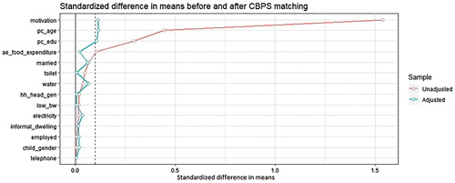
Figure A2. Standardised difference in means before and after matching under conventional

Bibliography

- Aguero, J, Carter, M & Woolard, I, 2006. The impact of unconditional cash transfers on nutrition: The South African Child Support Grant. Southern Africa labour & development research unit Working paper.
- Austin, PC, 2009. Balance diagnostics for comparing the distribution of baseline covariates between treatment groups in propensity-score matched samples. Statistics in Medicine 28(25), 3083–107. doi: 10.1002/sim.3697
- Bhattacharya, J & Vogt, WB, 2007. Do instrumental variables belong in propensity scores? NBER working paper.
- Boersma, B & Wit, JM, 1997. Catch-up growth. Endocrine Reviews 18(5), 646–61. doi: 10.1210/edrv.18.5.0313
- Caliendo, M & Kopeinig, S, 2008. Some practical guidance for the implementation of propensity score matching. Journal of Economic Surveys 22(1), 31–72. doi: 10.1111/j.1467-6419.2007.00527.x
- Case, A, Hosegood, V & Lund, F 2005. The reach and impact of Child Support Grants: Evidence from KwaZulu-Natal. Development Southern Africa 22(4), 467–82. doi: 10.1080/03768350500322925
- Coetzee, M, 2011. Finding the Benefits: evaluating the impact of the South African child support grant. Economic Research Southern Africa. Working paper 230.
- Coetzee, M, 2013. Finding the Benefits: estimating the impact of The South African child support grant. South African Journal of Economics 81(3), 427–50. doi: 10.1111/j.1813-6982.2012.01338.x
- d’Agostino, G, Scarlato, M & Napolitano, S, 2017. Do cash Transfers Promote food Security? The case of the South African child support grant. Journal of African Economies 27(4), 430–456. doi: 10.1093/jae/ejx041
- Dehejia, RH & Wahba, S, 1999. Causal effects in nonexperimental studies: Reevaluating the evaluation of training programs. Journal of the American Statistical Association 94(448), 1053–62. doi: 10.1080/01621459.1999.10473858
- Dehejia, RH & Wahba, S, 2002. Propensity score-matching methods for nonexperimental causal studies. Review of Economics and Statistics 84(1), 151–61. doi: 10.1162/003465302317331982
- Delany, A, Ismail, Z, Graham, L & Ramkissoon, Y, 2008. Review of the child support grant: Uses, implementation and obstacles. CASE, Johannesburg.
- Desmond, C & Casale, D, 2017. Catch-up growth in stunted children: Definitions and predictors. PloS one 12(12), e0189135. doi: 10.1371/journal.pone.0189135
- Diamond, A & Sekhon, JS, 2013. Genetic matching for estimating causal effects: A general multivariate matching method for achieving balance in observational studies. Review of Economics and Statistics 95(3), 932–945. doi: 10.1162/REST_a_00318
- Duflo, E, 2003. Grandmothers and granddaughters: Old-age pensions and intrahousehold allocation in South Africa. The World Bank Economic Review 17(1), 1–25. doi: 10.1093/wber/lhg013
- Hainmueller, J, 2012. Entropy balancing for causal effects: A multivariate reweighting method to produce balanced samples in observational studies. Political Analysis 20(1), 25–46. doi: 10.1093/pan/mpr025
- Hainmueller, J & Xu, Y, 2013. Ebalance: A Stata package for entropy balancing. Journal of Statistical Software, 54(7). doi: 10.18637/jss.v054.i07
- Heinrich, C. et al., 2012. The South African child support grant impact assessment: Evidence from a survey of children, adolescents and their households. Department of Social Development, South African Social Security Agency and UNICEF. Available @ http://agris.fao.org/agris-search/search.do?recordID=QB2015105453
- Imai, K & Ratkovic, M, 2014. Covariate balancing propensity score. Journal of the Royal Statistical Society: Series B (Statistical Methodology) 76(1), 243–63. doi: 10.1111/rssb.12027
- Oyenubi, A, 2018. Quantifying balance for causal inference: An information theoretic perspective (Doctoral dissertation, University of Cape Town).
- Oyenubi, A, 2019. Who benefits from South African child support grant: The role of gender and birthweight. Economic Research Southern Africa. Working paper 781.
- Smith, JA & Todd, PE, 2005. Does matching overcome LaLonde's critique of nonexperimental estimators? Journal of Econometrics 125(1), 305–53. doi: 10.1016/j.jeconom.2004.04.011
- Walker, SP, Chang, SM, Wright, A, Osmond, C & Grantham-McGregor, SM, 2015. Early childhood stunting is associated with lower developmental levels in the subsequent generation of children. The Journal of Nutrition 145(4), 823–8. doi: 10.3945/jn.114.200261