Subjective wellbeing inequality in South Africa 2008–14: An unconditional quantile decomposition analysis

ABSTRACT

This study analyses the sources of reduction in subjective wellbeing (SWB) inequality in South Africa over the period 2008–14. The unconditional quantile regression decomposition of mean gap finds differences in the effect of covariates along the SWB distribution, underlining the relevance of going beyond mean-based decomposition. Fall in SWB inequality is due to the increased level of SWB on the left-hand side of the distribution and a reduced level in the upper end of the distribution. Greater access to public amenities such as electricity and flushing toilets among those on the lower SWB distribution and lower returns to relative income and good health among those on the upper SWB spectrum can be said to be the major reasons for decline in SWB inequality. While the trend in returns to race has contributed to lower SWB inequality, employment stands out starkly as increasing inequality through both endowment and coefficient effect.

KEYWORDS:

• Subjective wellbeing
• unconditional quantile regression
• recentred influence function

1. Introduction

Research on happiness is a growing field in economic development, embedded in the belief that human development needs to be measured not only on criterion of income and physical well-being but also on self-reported happiness, life satisfaction and subjective wellbeing (SWB). Studies on inequality, however, are still dominated by income rather than on the basis of happiness or SWB.¹ Moreover, there is increasing indication from aggregate level cross-country studies that income inequality and happiness inequality need not follow similar trends (Veenhoeven, 2005). Despite this, there are very few country-specific studies on the drivers of happiness inequality (Becchetti et al., 2014). The few exceptions that exist (Stevenson & Wolfers, 2008; Dutta & Foster, 2013; Becchetti et al., 2014; Niimi, 2018) are confined to developed country contexts.

Newman (2016) describes happiness inequality as ‘the psychological parallel to income inequality: how much individuals in a society differ in their self-reported happiness levels—or subjective well-being, as happiness is sometimes called by researchers’. According to Helliwell et al. (2017), well-being inequality may be as or more relevant than the more commonly used measures of inequality in income and wealth. Veenhoven (2005) and Gandelman and Porzecanski (2013) found a decline in happiness inequality in cross-country studies. Country-specific studies such as those of Stevenson and Wolfers (2008), Clark et al. (2012) and Niimi (2018) found that happiness inequality decreased while income inequality increased in the US, Germany and Japan, respectively, while Becchetti et al. found an increase in happiness inequality and income inequality in Germany. The results of Becchetti et al. apart, the finding of decreasing happiness inequality in other country-specific studies contradicted the general notion of increasing income inequality.

While some country-specific studies such as those of Stevenson and Wolfers (2008) and Becchetti et al. decompose the source of the variation in the happiness gap between covariate and coefficient effects; these studies use decomposition methods (following Lemieux (2002) and Fortin et al. (2010), respectively) that do not differentiate decomposition over the different points of the SWB distribution. The limitation of this means-based approach is that uniform behaviour and response is assumed along the SWB distribution. This has been proven unrealistic by SWB studies using the quantile regression approach (Binder & Coad, 2010; Yuan & Golpelwar, 2013; Fang, 2017; Neira et al., 2019; Kollamparambil, 2020a). None of these studies, however, have attempted to decompose the quantile gaps. The decomposition of the SWB inequality gap by endowment effect and coefficient effect will provide a more nuanced understanding of the drivers of change. Therefore, this paper contributes to the literature by not only analysing happiness inequality in a developing country but also by undertaking an unconditional quantile regression decomposition to identify the contribution of coefficients and covariates to changes in SWB level over time at different points of the SWB distribution.

There is abundant South African literature on inequality, but it is based on income as opposed to subjective SWB. South Africa is a most suitable candidate country for the study of SWB inequality because, as well as the fact that its income-based Gini coefficients are reportedly the highest in the world, the 2018 World Happiness Report highlights South Africa as one of the least happy countries in the world, with a ranking of 105 out of 156 countries.

South African literature on SWB thus far is restricted to analysis of the trends and determinants of SWB levels (Moller, 1998, 2007; Hinks & Gruen, 2007; Posel & Casale, 2011; Blaauw & Pretorius, 2013; Kollamparambil, 2020a). Although some of these analyses delve into the differences in SWB levels across races (Moller, 1998, 2007; Hinks & Gruen, 2007; Posel & Casale, 2011), only Kollamparambil (2020a) addresses the overall trends and drivers of happiness inequality in South Africa. Kollamparambil (2020b) undertakes a comparative study of South Africa and Switzerland using the decomposition of concentration indices but fails to include key variables relevant to the South African context such as access to public amenities.

The objective of this paper is therefore to comprehend the recent trend of happiness inequality in South Africa using the first and fourth waves of the National Income Dynamics Survey, conducted in 2008 and 2014, respectively, and to identify the source of this trend along the SWB distribution. For this purpose, the paper goes beyond mean-based Oaxaca–Blinder decomposition and undertakes a decomposition of the mean gap over the SWB distribution as well as changes in inequality measures such as Gini, variance and inter-quantile ratios to identify drivers of happiness inequality.²

2. Literature review

We investigate our primary concern of inequality through the dispersion of happiness by first identifying the differences in the drivers of happiness at different levels of SWB distribution. Therefore, literature on determinants of happiness is the starting point for the analysis.

Much research has explored the relationship between income and happiness, reviewed effectively by Clark et al. (2008). Studies reveal that, while individual happiness is affected by income level (absolute effect), a person’s happiness is also affected by how they rate themself compared to others (relative effect). Van Praag (2011) formulated this in a theoretical model to argue that subjective well-being (SWB) does not depend on characteristics of the individual alone but also on characteristics of the individual’s reference group.

Dolan et al. (2008) provides an exhaustive review of the literature on other determinants of happiness, highlighting that poor health, separation, unemployment and lack of social contact are all strongly negatively associated with happiness. We draw upon the above literature for the inclusion of control variables in our analysis. Moreover, we include access to amenities like flushing toilets, electricity and so on, which are pertinent issues in a developing country like South Africa.

The investigation of happiness dispersion began with a cross-country study by Veenhoven (1990), who found happiness inequality to be different amongst nations, with happiness more equally distributed in democratically and economically developed nations characterised by minor income variances, high social security and equal educational chances. These properties were more noticeable in the rich than the developing countries. This study of happiness inequality was based solely on the analysis of trends without delving into its drivers. Veenhoven (2005), based on cross-country analysis, found that income inequality is not strongly related to life satisfaction inequality. The micro-data-based single-country studies on happiness inequality have utilised quantile regression and recentred influence function (RIF) regression estimation for identifying the drivers of happiness inequality (Stevenson & Wolfers, 2008; Clark et al., 2012; Becchetti et al., 2014; Niimi, 2018).

Niimi (2018) identified the major contributors to happiness inequality in Japan using RIF regression but did not undertake a decomposition of inequality gaps. Likewise, Kollamparambil (2020a) used RIF to identify the drivers of inequality in South Africa but does not take it forward to decompose the inequality measures. Stevenson and Wolfers (2008), in a time-series study of the US using Lemieux’s (2002) decomposition over the period 1972–2006, found that, while aggregate happiness levels have not increased, happiness gaps on lines of race and gender may have disappeared but the gap has widened by education. Becchetti et al. (2014), on the other hand, found an increase in happiness inequality over the period 1992–2007 in Germany and, through a decomposition analysis based on Fortin et al. (2010), that the dynamics of happiness inequality are explained by the composition effect rather than by the coefficient effect of covariates. According to the study, deteriorating labour market conditions and the middle-age cohort have contributed to rising happiness inequality, while education has an inequality reducing impact. Both the decomposition studies relied on mean-based methodology and did not undertake decomposition over the SWB distribution. The distribution-based methodology adopted by this study contributes to a better understanding of happiness inequality.

This study therefore is original in not only being the first to study happiness inequality within a developing country but also by making use of the unconditional quantile regression decomposition technique to comprehend the composition versus coefficient effects along the SWB distribution.

3. Data and methodology

The analysis uses National Income Dynamics Study (NIDS) data. NIDS is South Africa’s first national household panel study to collects information on people’s livelihoods and well-being, household composition and structure; fertility and mortality; migration; labour market participation and economic activity; human capital formation, health and education; and vulnerability and social capital. The survey commenced in 2008 with a countrywide representative sample of over 28 000 people in 7300 households across the country. The survey is conducted every two years; wave 1 commenced in 2008, followed by waves 2, 3 and 4 in 2010, 2012 and 2014, respectively. This study uses the first and fourth waves of the survey. Further sample weights are included to correct the sample representation in the NIDS data to account for attrition bias. The subjective well-being question included in the survey is: What is your current level of life satisfaction rated between one and ten? One is the least level of satisfaction and 10 is the highest.

Subjective SWB inequality measures, like other inequality measures, has many tools. According to Kalmjin and Veenhoven (2005), standard deviation or variance is a better measure of SWB inequality because of the bounded nature of SWB measurement on a scale of 1–10. We nevertheless analyse the trend as well as decomposition of SWB inequality changes over 2008–14 with various inequality measures such as Gini, variance and inter-quantile ratios for purposes of comparison.

The paper will follow Becchetti et al.’s (2014) and Niimi’s (2018) approach and select variables as informed by SWB literature for the quantile estimations on SWB. The study makes use of the following commonly identified determinants of SWB inequality: age, gender, race, health status, income level, relative income perception, education, marital status, employment status, access to bank credit, geographic type of residence (urban/rural), access to amenities like flushing toilets and electricity, religiosity and so on. Detailed variable definitions are provided in the Appendix.

As a first step, we decompose SWB inequality at the means over the two time points using the Blinder–Oaxaca approach. Oaxaca (1973) and Blinder (1973) introduced a decomposition procedure that enabled the attribution of the SWB gap of two time periods to composition effect and coefficient effect (Kollamparambil & Razak 2016):(1) $y_i^{2008}={\alpha }^{2008}+{\text{β}}^{2008}{x}_i^{2008}+{\epsilon }_i^{2008}$(1) (2) $y_i^{2014}={\alpha }^{2014}+{\text{β}}^{2014}{x}_i^{2014}+{\epsilon }_i^{2014}$(2) where y is the dependent variable and x is a vector of regressors.

The decomposition is calculated by subtracting the two equations, which yields:(3) $Y^{2014}-Y^{2008}={\text{β}}^{2014}\left(X^{2014}-X^{2008}\right)+\left({\alpha }^{2014}-{\alpha }^{2008}\right)+\left({\text{β}}^{2014}-{\text{β}}^{2008}\right)X^{2008}$(3) Where Y is the mean dependent variable and X is the mean of regressors. From equation 3, ${\text{β}}^{2014}\left(X^{2014}-X^{2008}\right)$ is the ‘explained’ portion of the gap. It is the SWB gap attributable to the differences in mean observable characteristics between 2008 and 2014. $\left({\alpha }^{2014}-{\alpha }^{2008}\right)+\left({\text{β}}^{2014}-{\text{β}}^{2008}\right)X^{2008}$ is the ‘unexplained’ portion, i.e. the differences in constant and coefficient estimates. This is the SWB disparity that would still remain if the data for people in 2014 displayed the average characteristics of people in 2008. The total gap at means between 2014 and 2008 is the sum of the observable characteristics (or endowment) portion and returns (or coefficient) portion.

According to Appleton et al. (2014), quantile regression analysis is a better approach for studying inequality because we are concerned with the entire distribution as opposed to the midpoint of the distribution. Binder and Coad (2010) argued that a normal ordinary least squares regression (OLS) does not provide a holistic picture of the relationship between SWB and its determinants. The literature has indicated that the effect of and response to covariates vary along the SWB distribution (Binder & Coad, 2010; Yuan & Golpelwar, 2013; Fang, 2017; Neira et al., 2019; Kollamparambil, 2020a).

Using the RIF method developed by Firpo et al. (2009), this study estimates unconditional quantile regressions. Unlike the conditional quantile regression, unconditional quantile regression can be used to estimate the impact of a covariate on the corresponding unconditional quantile. Therefore to determine the differences in the drivers of SWB levels at different segments of the SWB distribution, we first run unconditional quantile regressions (p = 10, 25, 50, 75 and 90, t = 2008/2014) using the robust OLS regression for the two time points separately.$\begin{array}{rl}SW{B}_{qt}& ={\text{β}}_0+{\text{β}}_{1}Incom{e}_{qt}+{\text{β}}_{2}Ag{e}_{qt}+{\text{β}}_{3}Ag{e}_{qt}^2+{\text{β}}_{4}Femal{e}_{qt}\\ & +{\text{β}}_{5}Marrie{d}_{qt}+{\text{β}}_{6}Abovematri{c}_{qt}+{\text{β}}_{7}Health{y}_{qt}+{\text{β}}_{8}Employe{d}_{qt}\\ & +{\text{β}}_{9}Relatively\mathrm{\_}ric{h}_{qt}+{\text{β}}_{10}Bankloa{n}_{qt}+{\text{β}}_{11}Flushingtoile{t}_{qt}\\ & +{\text{β}}_{12}Electricit{y}_{qt}+{\text{β}}_{13}Urba{n}_{qt}+{\text{β}}_{14}Blac{k}_{qt}+{\text{β}}_{15}Religiou{s}_{qt}+{\mu }_{qt}\end{array}$

Unconditional quantile regression aside, the RIF method can be used to replace the dependent variable of a regression with the distributional statistics of interest corresponding to the recentred influence function (Clark et al., 2012; Becchetti et al., 2014; Niimi, 2018; Kollamparambil, 2020a). Accordingly, in order to study inequality, the study uses RIF to estimate the effect of changes in covariates on the variance, and the Gini coefficient. The coefficients of the RIF regressions are interpreted similarly to the ordinary least squares regression, that is, by how much the function of the marginal outcome distribution is affected by an infinitesimal shift to the right in the distribution of the regressors (Kollamparambil, 2020a). Oaxaca–Blinder decompositions can be used in combination with RIFs to analyse decompositions of any distributional statistic for which an RIF can be calculated (Firpo et al., 2018). This study uses the oaxaca_rif wrapper program in Stata to compute the Oaxaca–Blinder (BO) decomposition of the mean gap at various percentiles and for changes in various inequality measures over time.

3.1. Preliminary analysis

Table 1 shows that average SWB increased over the period of analysis. The inflation-adjusted per capita household income also shows an improvement over the period, highlighting the close association between income and SWB. However, the standard deviations indicate growing income inequality and declining SWB inequality.

Table 1. Summary descriptive statistics.

	Period1			Period 2
Variable	Obs	Mean	SD	Obs	Mean	SD
SWB (1–10 scale)	3906	4.899	2.456	4682	5.022	2.274
Income per capita, rand	3906	785.60	1681.53	4682	1793.8	3371.8
Age (years)	3906	38.320	16.966	4682	45.120	16.869
Female (0/1)	3906	0.672	0.470	4682	0.664	0.472
Married (0/1)	3906	0.271	0.444	4682	0.291	0.454
Employed (0/1)	3906	0.358	0.480	4682	0.412	0.492
Relatively rich (0/1)	3906	0.135	0.342	4682	0.184	0.387
Above matriculation (0/1)	3906	0.047	0.212	4682	0.101	0.302
Good health (0/1)	3906	0.904	0.295	4682	0.955	0.207
Bank loan (0/1)	3906	0.022	0.148	4682	0.054	0.227
Urban (0/1)	3906	0.409	0.492	4682	0.489	0.500
Flushing toilet	3906	0.376	0.484	4682	0.462	0.499
Electricity (0/1)	3906	0.707	0.455	4682	0.849	0.358
Black (0/1)	3906	0.870	0.337	4682	0.857	0.350
Religious (0/1)	3906	0.903	0.296	4682	0.920	0.271

Source: NIDS weighted sample calculation.

The proportion of individuals who perceived their relative income to be not below average (relatively rich) also increased between the periods. Alongside this, increased access to amenities such as bank credit, electricity and flushing toilets can be seen in the second period. The positive correlation between SWB and these variables is indicated by the common trend observed.

The average age in both periods is upper thirties, which is slightly above the youth age category in South Africa. This is reflective of South Africa’s young population. South Africa, like most African countries, has a young population; hence, it is not surprising to find such an age distribution. There are more females than males in South Africa and the sample represents this statistic; however, the female population appears nevertheless to be over-represented in the sample in both periods. The sample reflects the low level of education in South Africa, with only 10% reporting a qualification above Grade 12 (above matriculation), although the level had almost doubled by 2014. The sample shows employment rates of between 36–41% in 2008 and 2014, respectively. The majority of the South African population is black, which is represented in the sample. South Africa is a religious country and the sample reflects that: 90 and 92% of people in 2008 and 2014, respectively, identified religion as important. An improvement in health status is evident between the years.

The spatial centralisation of development in many emerging countries has resulted in rural–urban migration and this is reflected in urban dwellers increasing from 40 to 49% in the sample. The low access to bank credit is reflective of the South African context, whereby many people cannot access formal sector credit. Although there has been a substantial increase in accessing bank credit, the proportion still remains very low.

Table 2 shows that total SWB inequality based on all measures of inequality is declining. The decreasing SWB inequality is in line with the findings of Kollamparambil (2020a) in the South African context and other studies in various country contexts such as Stevenson and Wolfers (2008), Clark et al. (2012) and Gandelman and Porzecanski (2013). However, Becchetti et al. found an increase in happiness inequality in Germany.

Table 2. SWB inequality.

	2008	2014
Percentile ratios	6.86	6.16
p90/p10
p75/p25	3.35	3.27
p90/p50	3.76	3.36
p50/p10	3.10	2.8
Variance	6.03	5.17
Gini	0.28	0.25

Source: NIDS weighted sample-based estimation.

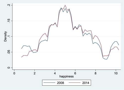
Overall, SWB inequality can decrease in two ways; either: (1) SWB for those who were least happy increased while SWB of others remained unchanged or (2) SWB of the happier individuals deteriorated while it remained unchanged for others. The comparison of percentile measures of SWB inequality indicate that SWB at the lower half of the distribution has improved substantially resulting in lower SWB inequality over the period. Reduced inequality in 2014 is clearly evident from the reductions on both extremes of the density distribution. There is an increased density to the right-hand side of the lower tail and the left-hand side of the upper tail (Figure 1). The median is also higher in 2014 compared to 2008.

Figure 1. Distribution of SWB in 2008 and 2014.

4. RIF regression results

It is clear from our results (Tables 3 and 4) that substantial variation exists in the impact of covariates at different percentiles. While per capita household income is unequivocally associated with more SWB, being black clearly leads to less SWB at all percentiles in both periods. The positive relationship between household income is in line with previous studies of SWB determinants (Kollamparambil, 2020a). The significance of income across all percentiles differs from the results of Binder and Coad (2010), who found that income is effectively significant at all percentiles except the 90th decile of SWB distribution in Britain.

Table 3. Unconditional quantile regression: 2008, dependent variable: SWB level.

Percentile	rif_10	rif_25	rif_50	rif_75	rif_90
Variables
Income (log)	0.185**	0.159***	0.247***	0.197**	0.326***
	(0.0758)	(0.0565)	(0.0523)	(0.0871)	(0.111)
Age	−0.0118	−0.0476***	−0.0512***	−0.0815***	−0.0812***
	(0.0197)	(0.0145)	(0.0142)	(0.0218)	(0.0259)
Age-squared	0.000214	0.000535***	0.000519***	0.000774***	0.000789***
	(0.000223)	(0.000163)	(0.000161)	(0.000245)	(0.000288)
Female	0.111	0.0911	−0.117	−0.189	−0.284
	(0.134)	(0.0982)	(0.0945)	(0.155)	(0.190)
Married	−0.230	0.140	0.270**	0.311*	0.268
	(0.149)	(0.110)	(0.105)	(0.169)	(0.206)
Employed	0.164	0.139	0.0191	0.0957	0.197
	(0.140)	(0.105)	(0.0990)	(0.158)	(0.194)
Relatively rich	0.678***	0.723***	1.574***	3.365***	3.028***
	(0.126)	(0.0952)	(0.116)	(0.249)	(0.329)
Above matriculation	0.494*	−0.302	0.0374	0.406	0.634
	(0.280)	(0.195)	(0.192)	(0.373)	(0.502)
Good health	0.773***	0.858***	0.781***	0.693***	0.711***
	(0.247)	(0.183)	(0.145)	(0.200)	(0.236)
Bank loan	0.226	0.290*	0.536**	0.234	−0.823
	(0.260)	(0.170)	(0.218)	(0.554)	(0.691)
Urban	−0.313*	−0.290**	−0.0879	−0.354*	−0.0911
	(0.179)	(0.140)	(0.134)	(0.211)	(0.251)
Flushing toilet	0.178	0.363**	0.308**	0.274	0.0191
	(0.196)	(0.154)	(0.150)	(0.236)	(0.278)
Electricity	0.623***	0.348***	0.279***	0.521***	0.398**
	(0.151)	(0.112)	(0.101)	(0.147)	(0.174)
Black	−0.731***	−0.772***	−1.548***	−1.863***	−2.184***
	(0.145)	(0.105)	(0.122)	(0.254)	(0.329)
Religious	0.1609	0.367**	0 .516***	0.472**	0.354
	(0.212)	(0.160)	(0.149)	(0.231)	(0.268)
Constant	0.504	2.924***	4.884***	8.027***	9.340***
	(0.666)	(0.481)	(0.471)	(0.782)	(0.965)
Observations	3906	3906	3906	3906	3906
R^2	0.028	0.052	0.143	0.128	0.090

Robust standard errors in parentheses. *** p < 0.01, ** p < 0.05, * p < 0.1.

Table 4. Unconditional quantile regression: 2014, dependent variable: SWB level.

Percentile	rif_10	rif_25	rif_50	rif_75	rif_90
Variables
Income (log)	0.064**	0.0806**	0.226***	0.308***	0.198**
	(0.031)	(0.0409)	(0.0438)	(0.0733)	(0.0775)
Age	−0.0159	−0.0129	−0.0353***	−0.0688***	−0.0686***
	(0.0130)	(0.0119)	(0.0122)	(0.0197)	(0.0204)
Age-squared	0.000166	0.000135	0.000374***	0.000731***	0.000805***
	(0.000133)	(0.000120)	(0.000123)	(0.000199)	(0.000209)
Female	−0.0184	−0.00533	0.139*	0.0858	0.112
	(0.0774)	(0.0722)	(0.0759)	(0.124)	(0.126)
Married	0.0311	0.210***	0.331***	0.280**	0.271**
	(0.0859)	(0.0746)	(0.0801)	(0.133)	(0.138)
Employed	−0.118	−0.0799	0.208***	0.411***	0.527***
	(0.0871)	(0.0768)	(0.0788)	(0.128)	(0.131)
Relatively rich	−0.0982	−0.219**	−0.714***	−0.195	−0.0717
	(0.0985)	(0.0930)	(0.0878)	(0.144)	(0.150)
Above matriculation	0.195*	0.262**	0.488***	0.397*	0.399*
	(0.104)	(0.103)	(0.118)	(0.213)	(0.222)
Good health	0.623***	0.363**	0.122	−0.457	−0.476
	(0.233)	(0.180)	(0.166)	(0.280)	(0.300)
Bank loan	0.126	0.0511	0.208	0.209	0.352
	(0.151)	(0.137)	(0.151)	(0.279)	(0.305)
Urban	−0.0529	−0.0125	−0.181*	−0.0863	−0.00772
	(0.112)	(0.0986)	(0.101)	(0.160)	(0.159)
Flushing toilet	0.129***	0.208**	0.461***	0.708***	0.543***
	(0.018)	(0.103)	(0.108)	(0.172)	(0.172)
Electricity	0.526***	0.224**	0.125	0.142	0.0656
	(0.129)	(0.106)	(0.101)	(0.151)	(0.149)
Black	−0.504***	−0.532***	−0.538***	−1.226***	−1.443***
	(0.0826)	(0.0735)	(0.104)	(0.194)	(0.215)
Religious	0 .149	0 .199	0 .071	0 .641***	0 .609***
	(0.152)	(0.139)	(0.136)	(0.204)	(0.203)
Constant	1.790***	3.123***	4.374***	6.818***	9.267***
	(0.501)	(0.442)	(0.473)	(0.789)	(0.819)
Observations	4682	4682	4682	4682	4682
R^2	0.016	0.024	0.056	0.056	0.053

Robust standard errors in parentheses. *** p < 0.01, ** p < 0.05, * p < 0.1.

The shifting relevance of a range of variables over time is also apparent. Variables such as urban, flushing toilets and electricity showed considerable changes over the period 2008–14. Electricity impacted all percentiles positively in 2008 but in 2014 impacted only lower percentiles significantly. Flushing toilets, on the other hand, were more relevant in 2014 than in 2008. The importance of being religious has also shifted along the distribution curve; it positively impacted SWB at the mid-percentiles in 2008 and at the 75th and90th percentiles in 2014.

The U-shape relationship between age and SWB is evident except at the lower percentiles in both 2008 and 2014. The impact of being married has increased over time; it had a positive and significant impact on more percentiles in 2014 compared to only the median and 75th percentile in 2008. The relevance of a bank loan, on the other hand, has declined, with none of the percentiles showing a significant impact in 2014. The increasing relevance of higher education across the percentile spectrum in 2014 is very noticeable. Being employed has also become highly relevant in 2014 at the higher percentiles. The relevance of good health has declined over time and is significant only among the lower percentiles in 2014. It is, however, surprising that being female does not affect SWB level significantly in either time period, except for the 50th percentile in the second period.

For a more direct understanding of the covariates of SWB inequality, we present the RIF using the Gini and variance measures of inequality (Table 5). The Gini coefficient is a bounded measure of inequality ranging from zero to one, while variance is not bounded; as such, a comparison between the two is difficult. According to Kalmjin and Veenhoven (2005), variance is preferred over other measures of inequality such as Gini given the bounded nature of our measurement of SWB. Nevertheless, we present estimations based on both measures of inequality for the purpose of comparison. A substantial difference appears to exist in the contribution of covariates based on Gini and variance. While household income has a negative and significant association with Gini, its association with the variance measure of inequality is not significant. On the other hand, black has a positive correlation with Gini but a negative association with variance. While relatively rich has a negative and significant association with Gini in 2008, it has changed to positive and significant in 2014 in line with variance. However, it is worth noting that electricity and good health have negative and significant associations across both inequality measures.

Table 5. Recentred influence function regression: Gini, variance.

	(2008)	(2014)	(2008)	(2014)
Variables	Gini	Gini	Variance	Variance
Income (log)	−0.0102***	−0.00702**	0.0370	0.0621
	(0.00390)	(0.00338)	(0.149)	(0.121)
Age	0.000994	0.000878	−0.0736*	−0.0377
	(0.000998)	(0.000915)	(0.0381)	(0.0327)
Age-squared	−1.46e-05	−7.58e-06	0.000557	0.000486
	(1.13e-05)	(9.20e-06)	(0.000430)	(0.000329)
Female	−0.00406	0.000498	−0.447*	0.138
	(0.00687)	(0.00571)	(0.262)	(0.204)
Married	−0.00371	−0.0132**	0.0903	0.0830
	(0.00777)	(0.00611)	(0.296)	(0.219)
Employed	−0.00319	0.0101*	0.0583	0.754***
	(0.00719)	(0.00594)	(0.274)	(0.212)
Relatively rich	−0.0203**	0.0334***	2.524***	0.415*
	(0.00958)	(0.00697)	(0.366)	(0.249)
Above matriculation	0.0249	−0.0272***	1.078*	−0.311
	(0.0154)	(0.00928)	(0.586)	(0.332)
Good health	−0.0606***	−0.0519***	−0.879**	−1.984***
	(0.0108)	(0.0126)	(0.413)	(0.451)
Bank loan	−0.0316	−0.00343	−0.817	0.403
	(0.0216)	(0.0119)	(0.825)	(0.424)
Urban	0.0121	0.00766	0.190	0.0720
	(0.00975)	(0.00762)	(0.372)	(0.272)
Flushing toilet	−0.0192*	−0.0127	−0.336	0.386
	(0.0107)	(0.00809)	(0.409)	(0.289)
Electricity	−0.0231***	−0.0262***	−0.239**	−0.731***
	(0.00718)	(0.00743)	(0.074)	(0.266)
Black	0.0401***	0.0150*	−1.160***	−1.085***
	(0.0101)	(0.00808)	(0.386)	(0.289)
Religious	−0.0254**	−0.00305	−0.182	0.424
	(0.0106)	(0.00963)	(0.406)	(0.344)
Constant	0.401***	0.342***	9.715***	7.661***
	(0.0343)	(0.0356)	(1.310)	(1.274)
Observations	3910	4675	3910	4675
R^2	0.035	0.019	0.023	0.018

Standard errors in parentheses. *** p < 0.01, ** p < 0.05, * p < 0.1.

5. Decomposition of the SWB mean gap

As discussed in the methodology section, change in SWB inequality can be counterfactually decomposed into that attributable to changes in the composition of covariates of the regressions and that which is attributable to changes in the coefficient or returns to covariates. Before undertaking the decomposition of changes along various segments of the SWB distribution, as well as the inequality statistics, we first undertake Oaxaca–Blinder decomposition of the mean gap over the period 2008–14.

The SWB gap of 0.123 indicates an increase in SWB over the period 2008–14 (Table 6). The increase in average SWB is explained by the endowment effect of the following variables: household income, above matriculation, good health, relatively rich, black, married and employed. Improved access to public amenities such as electricity, flushing toilets and bank loans have also contributed to the increase in SWB. Among the coefficient effects, black, female and flushing toilet variables have contributed significantly to increasing the level of SWB in 2014. The findings of the study with regard to black therefore differ from those of Stevenson and Wolfers (2008), who found, in the US context, that the decline in SWB gap in gender and race can be attributed to the covariates rather than the changed structure of SWB. The returns to other covariates such as relatively rich and good health are seen to contribute to mitigating the increase in SWB levels in 2014. Overall, however, the positive endowment effect outweighs the negative coefficient effect in our decomposition analysis at the means. Next, we undertake the Oaxaca–Blinder decomposition along the SWB distribution and inequality statistics using RIF regressions.

Table 6. Oaxaca–Blinder decomposition of SWB mean gap across 2014–08.

	(1)	(2)	(3)	(4)	(5)
Variables	OLS 2008	OLS 2014	overall	Explained	unexplained
Income (log)	0.198***	0.192***		0.105***	−0.0444
	(0.0471)	(0.0415)		(0.0173)	(0.425)
Age	−0.0514***	−0.0404***		−0.379***	0.526
	(0.0119)	(0.0115)		(0.0585)	(0.688)
Age-squared	0.000514***	0.000439***		0.327***	−0.211
	(0.000132)	(0.000117)		(0.0520)	(0.354)
Female	−0.146*	0.0700		0.000218	0.144**
	(0.0832)	(0.0714)		(0.000507)	(0.0731)
Married	0.129	0.299***		0.00457*	0.0475
	(0.0889)	(0.0766)		(0.00251)	(0.0327)
Employed	0.0850	0.221***		0.00929***	0.0514
	(0.0864)	(0.0751)		(0.00358)	(0.0437)
Relatively rich	1.668***	−0.449***		0.0183***	−0.327***
	(0.112)	(0.0846)		(0.00461)	(0.0232)
Above matriculation	0.0878	0.411***		0.0147***	0.0229
	(0.185)	(0.114)		(0.00553)	(0.0139)
Good health	0.697***	−0.0207		0.0246***	−0.674***
	(0.124)	(0.181)		(0.00604)	(0.206)
Bank loan	0.221	0.250		0.00815*	0.000502
	(0.219)	(0.156)		(0.00427)	(0.00843)
Urban	−0.156	−0.120		−0.00959	0.0149
	(0.112)	(0.0932)		(0.00594)	(0.0645)
Flushing toilet	0.192	0.476***		0.0301***	0.117*
	(0.125)	(0.0990)		(0.00771)	(0.0655)
Electricity	0.320***	0.160*		0.0402***	−0.131
	(0.0846)	(0.0958)		(0.00944)	(0.101)
Black	−1.304***	−0.869***		0.0135*	0.376***
	(0.117)	(0.105)		(0.00805)	(0.136)
Religious	0.394***	0.303**		0.00576**	−0.0831
	(0.129)	(0.120)		(0.00259)	(0.160)
Group_1			5.022***
			(0.0333)
Group_2			4.899***
			(0.0393)
Difference			0.123**
			(0.0515)
explained			0.213***
			(0.0253)
unexplained			−0.0906*
			(0.0525)
Constant	4.383***	4.462***			0.0783
	(0.431)	(0.451)			(0.623)
Observations	3910	4675	8585	8585	8585
R^2	0.160	0.076

Robust standard errors in parentheses. *** p < 0.01, ** p < 0.05, * p < 0.1

6. Oaxaca–Blinder decomposition of SWB inequality gaps

The average SWB level is higher in 2014 than in 2008 across percentiles, except at the highest percentile (Table 7). The lower percentiles have lower average levels of SWB but show the highest increase over 2008–14. This points to decreasing overall SWB inequality across percentiles over the period 2008–14. The Oaxaca–Blinder decomposition shows that, while at the lowest percentile (10th) both endowment and coefficient effects have contributed to the increase in SWB level, at the middle percentiles the increase in average SWB over time emanates primarily from the endowment effect. On the other hand, at the higher percentiles (75th and 90th) the coefficient effect contributes to reducing the SWB level. At the highest percentile the positive endowment effect of increasing SWB is overcompensated by the negative coefficient effect, resulting in reduced levels of SWB in 2014.

Table 7. Decomposition of SWB gaps: unconditional quantile regressions, across Group1–2014 and Group 2–2008.

Percentile	10		25		50		75		90
Variables	explained	unexplainededed	Explained	unexplained	explained	unexplained	explained	unexplained	explained	unexplained
Income (log)	0.154**	−0.851	0.133***	−0.528	0.209***	−0.0391	0.163**	0.901	0.280***	−0.872
	(0.0644)	(0.614)	(0.0484)	(0.504)	(0.0453)	(0.499)	(0.0752)	(0.826)	(0.0959)	(0.983)
Age	−0.0835	−0.265	−0.328***	1.524*	−0.359***	0.626	−0.569***	0.388	−0.564***	0.283
	(0.134)	(1.087)	(0.101)	(0.883)	(0.100)	(0.891)	(0.154)	(1.386)	(0.182)	(1.562)
Age-squared	0.124	−0.0694	0.306***	−0.907*	0.302***	−0.283	0.448***	−0.000955	0.455***	0.205
	(0.126)	(0.613)	(0.0948)	(0.488)	(0.0946)	(0.494)	(0.143)	(0.762)	(0.168)	(0.864)
Female	−0.000541	−0.0668	−0.000325	−0.0388	0.00146	0.222***	0.00217	0.239*	0.00261	0.293*
	(0.00124)	(0.105)	(0.000861)	(0.0842)	(0.00212)	(0.0842)	(0.00320)	(0.137)	(0.00386)	(0.158)
Married	−0.00494	0.0848*	0.00255	0.0313	0.00520	0.0299	0.00596	0.00342	0.00515	0.0133
	(0.00384)	(0.0509)	(0.00256)	(0.0401)	(0.00332)	(0.0404)	(0.00452)	(0.0652)	(0.00492)	(0.0754)
Employed	0.00904	−0.121*	0.00749	−0.0910	0.000922	0.0880	0.00562	0.139	0.0112	0.154
	(0.00781)	(0.0696)	(0.00594)	(0.0559)	(0.00548)	(0.0550)	(0.00879)	(0.0876)	(0.0109)	(0.101)
Relatively rich	0.0331***	−0.145***	0.0353***	−0.178***	0.0778***	−0.441***	0.166***	−0.673***	0.150***	−0.588***
	(0.00813)	(0.0304)	(0.00739)	(0.0262)	(0.0139)	(0.0311)	(0.0296)	(0.0584)	(0.0293)	(0.0710)
Above matriculation	−0.0270*	0.0718**	−0.0167	0.0603***	0.00194	0.0512**	0.0233	−0.000365	0.0374	−0.0250
	(0.0154)	(0.0306)	(0.0109)	(0.0232)	(0.0106)	(0.0239)	(0.0208)	(0.0450)	(0.0281)	(0.0575)
Good health	0.0396***	−0.0982	0.0448***	−0.450*	0.0409***	−0.617***	0.0362***	−1.166***	0.0373***	−1.212***
	(0.0135)	(0.336)	(0.0107)	(0.258)	(0.00885)	(0.225)	(0.0113)	(0.349)	(0.0131)	(0.391)
Bank loan	0.00707	−0.00482	0.00916	−0.0128	0.0171**	−0.0165	0.00693	−0.000610	−0.0278	0.0672
	(0.00843)	(0.0167)	(0.00568)	(0.0125)	(0.00752)	(0.0152)	(0.0182)	(0.0348)	(0.0229)	(0.0426)
Urban	−0.0252*	0.126	−0.0234**	0.135	−0.00720	−0.0506	−0.0296*	0.132	−0.00801	0.0407
	(0.0148)	(0.106)	(0.0118)	(0.0872)	(0.0110)	(0.0859)	(0.0177)	(0.135)	(0.0205)	(0.151)
Flushing toilet	0.0155	−0.141	0.0316**	−0.0602	0.0270**	0.0874	0.0237	0.225	0.00117	0.271*
	(0.0170)	(0.108)	(0.0139)	(0.0888)	(0.0135)	(0.0890)	(0.0208)	(0.140)	(0.0243)	(0.158)
Electricity	0.0864***	−0.0537	0.0484***	−0.0859	0.0369**	−0.112	0.0706***	−0.303	0.0552**	−0.281
	(0.0220)	(0.173)	(0.0163)	(0.137)	(0.0148)	(0.128)	(0.0218)	(0.188)	(0.0256)	(0.205)
Black	0.00905	0.162	0.00968	0.169	0.0196*	0.836***	0.0234	0.475*	0.0277	0.548
	(0.00567)	(0.145)	(0.00591)	(0.114)	(0.0117)	(0.144)	(0.0143)	(0.285)	(0.0170)	(0.352)
Religious	0.00269	−0.00225	0.00622*	−0.144	0.00881**	−0.414**	0.00804*	0.193	0.00604	0.280
	(0.00388)	(0.256)	(0.00368)	(0.210)	(0.00411)	(0.193)	(0.00476)	(0.278)	(0.00503)	(0.306)
Constant		1.524*		0.503		−0.154		−0.840		0.183
		(0.838)		(0.682)		(0.707)		(1.160)		(1.327)
Group_1 2014	2.538***		3.832***		5.340***		7.104***		8.704***
	(0.0384)		(0.0360)		(0.0382)		(0.0612)		(0.0634)
Group_2 2008	2.048***		3.639***		5.144***		7.007***		8.878***
	(0.0597)		(0.0459)		(0.0465)		(0.0734)		(0.0874)
Difference	0.490***		0.193***		0.196***		0.0975		−0.174**
	(0.0710)		(0.0583)		(0.0602)		(0.0955)		(0.08)
explained	0.339***		0.266***		0.382***		0.385***		0.468***
	(0.0624)		(0.0461)		(0.0494)		(0.0835)		(0.103)
unexplained	0.150*		−0.0732		−0.187***		−0.287**		−0.642***
	(0.0834)		(0.0674)		(0.0717)		(0.122)		(0.149)
2008 obs	3906		3906		3906		3906		3906
2014 obs	4682		4682		4682		4682		4682

Standard errors in parentheses. *** p < 0.01, ** p < 0.05, * p < 0.1.

At the lowest (10th) percentile, income, electricity, good health and relatively rich contribute to the positive endowment effect, while above matriculation and married contribute to an increase in SWB via the coefficient effect. The returns to employed and relatively rich, on the other hand, mitigate the increase marginally. At the 25th percentile, the endowment effect dominates the coefficient effect, although both contribute to an increase in SWB level in 2014. The main covariates explaining the increased SWB level via the endowment effect are income, relatively rich, electricity, flushing toilets, good health and religious. The urban variable has, however, reduced the total endowment effect. Among the coefficient effects, returns to age and above matriculation have led to an increase in SWB level in 2014, while relatively rich and good health have the opposite effect. The covariate drivers behind the endowment effect at the median percentile are similar to those at the 25th percentile, highlighting the important role of higher income as well as improved access to electricity, flushing toilets, higher education and more individuals being married. An important difference is the substantial coefficient effect of black in increased SWB levels. This is also noticeable at the 75th percentile.

The coefficient effect is larger than the endowment effect at the highest (90th) percentile and, as such, even though the endowment effect contributes to increased SWB level in 2014, the net effect is a decline in SWB level at the 90th percentile. The variables that contribute towards the endowment effect at lower percentiles are also seen to be significant at the higher percentiles. It is noticeable that the positive coefficient effect of female to increased SWB is significant only in the mid and upper percentiles.

While the quantile decomposition provides insights into the distributional differences, clearer insights into the contributors to declining SWB inequality can be obtained through the Oaxaca–Blinder decomposition of inequality gaps using various measures of inequality such as Gini, variance and inter-quantile ratios (Table 8). A decline in SWB inequality over the period 2008–14 is clearly evident across all inequality measures. While both endowment and coefficient effects are significant in the Gini decomposition, variance and extreme inter-quantile range (10/90) decomposition indicate the coefficient effect to be more relevant than the covariate effect in explaining the reduction in inequality. This is a departure from the results of Becchetti et al. (2014), who found that the change in SWB inequality in the US is due mainly to covariate composition and not coefficient effects. The result for Gini is more in line with what was described for the different percentiles (Table 7). The results for the variance, with the clear predominance of the coefficient effects, are in line with the ratio between the extreme percentiles (10/90), probably reflecting that the variance is much more sensitive to what happens at the extreme of the distribution. The Gini, on the other hand, uses the information from the entire distribution and is more aligned with the outcomes noted in the decomposition of the changes over time at various percentiles (Table 7).

Table 8. Oaxaca–Blinder decomposition of inequality gap: Group1–2014 and Group 2–2008.

	Gini		Variance		IQR 25/75		IQR10/90
Variables	explained	unexplained	explained	unexplained	explained	unexplained	explained	unexplained
Income (log)	−0.00543***	0.0227	0.0196	0.177	0.0198	1.438	0.0858	−0.116
	(0.00210)	(0.0358)	(0.0829)	(1.381)	(0.0516)	(0.902)	(0.0699)	(1.137)
Age	0.00676	−0.00525	−0.501**	1.623	−0.250	−1.075	−0.501**	0.682
	(0.00686)	(0.0617)	(0.255)	(2.246)	(0.168)	(1.505)	(0.217)	(1.823)
Age-squared	−0.00825	0.0164	0.314	−0.165	0.149	0.881	0.348*	0.204
	(0.00642)	(0.0341)	(0.234)	(1.231)	(0.157)	(0.831)	(0.201)	(1.015)
Female	3.02e-05	0.00302	0.00333	0.388*	0.00257	0.285*	0.00323	0.367**
	(6.60e-05)	(0.00594)	(0.00499)	(0.225)	(0.00375)	(0.147)	(0.00474)	(0.182)
Married	−7.47e-05	−0.00275	0.00182	−0.00212	0.00352	−0.0296	0.0102	−0.0731
	(0.000160)	(0.00287)	(0.00589)	(0.107)	(0.00422)	(0.0708)	(0.00705)	(0.0880)
Employed	−0.000172	0.00547	0.00315	0.287**	−0.00187	0.230**	0.00266	0.270**
	(0.000392)	(0.00389)	(0.0151)	(0.145)	(0.00965)	(0.0950)	(0.0127)	(0.118)
Relatively rich	−0.000984**	0.00986***	0.122***	−0.388***	0.135***	−0.510***	0.122***	−0.464***
	(0.000427)	(0.00198)	(0.0283)	(0.0888)	(0.0252)	(0.0585)	(0.0263)	(0.0750)
Above matriculation	0.00135	−0.00529***	0.0586	−0.141*	0.0411*	−0.0628	0.0653**	−0.0985
	(0.000824)	(0.00175)	(0.0360)	(0.0743)	(0.0218)	(0.0465)	(0.0313)	(0.0629)
Good health	−0.00312***	0.00831	−0.0453**	−1.055*	−0.00850	−0.717*	−0.000494	−1.146**
	(0.000696)	(0.0177)	(0.0210)	(0.626)	(0.0131)	(0.383)	(0.0171)	(0.483)
Bank loan	−0.00101*	0.00153	−0.0262	0.0663	−0.00223	0.0122	−0.0357	0.0735
	(0.000561)	(0.00112)	(0.0288)	(0.0553)	(0.0188)	(0.0359)	(0.0250)	(0.0461)
Urban	0.000966	−0.00216	0.0152	−0.0578	−0.00648	−0.000470	0.0166	−0.0813
	(0.000786)	(0.00604)	(0.0298)	(0.222)	(0.0194)	(0.149)	(0.0246)	(0.180)
Flushing toilet	−0.00164*	0.00299	−0.0288	0.333	−0.00796	0.286*	−0.0141	0.410**
	(0.000935)	(0.00617)	(0.0350)	(0.227)	(0.0229)	(0.153)	(0.0288)	(0.185)
Electricity	−0.00329***	−0.00256	−0.0339	−0.419	0.0232	−0.223	−0.0283	−0.245
	(0.00110)	(0.00954)	(0.0378)	(0.323)	(0.0245)	(0.210)	(0.0317)	(0.255)
Black	−0.000501	−0.0215**	0.0145	0.0644	0.0142	0.339	0.0197	0.458
	(0.000318)	(0.00969)	(0.0102)	(0.474)	(0.00906)	(0.292)	(0.0125)	(0.373)
Religious	−0.000423*	0.0205	−0.00303	0.558	0.00191	0.332	0.00359	0.269
	(0.000243)	(0.0141)	(0.00692)	(0.482)	(0.00434)	(0.314)	(0.00576)	(0.380)
Constant		−0.0621		−2.046		−1.378		−1.301
		(0.0496)		(1.921)		(1.258)		(1.540)
Group_1 (2014)	0.255***		5.170***		3.272***		6.166***
	(0.00258)		(0.0921)		(0.0633)		(0.0706)
Group_2 (2008)	0.282***		6.031***		3.352***		6.860***
	(0.00312)		(0.118)		(0.0780)		(0.101)
Difference	−0.0266***		−0.861***		−0.0801		−0.694***
	(0.00405)		(0.150)		(0.100)		(0.123)
explained	−0.0158***		−0.0851		0.113*		0.0985
	(0.00246)		(0.101)		(0.0660)		(0.0868)
unexplained	−0.0108**		−0.776***		−0.193		−0.793***
	(0.00443)		(0.179)		(0.118)		(0.148)
2008 obs	3906		3906		3906		3906
2014 obs	4682	.	4682	.	4682	.	4682	.

Standard errors in parentheses. *** p < 0.01, ** p < 0.05, * p < 0.1.

Among the endowment effects, increased income level, individuals considering themselves to be relatively rich and in good health, with access to bank loans, flushing toilets and electricity, have contributed to reduced Gini over the period. Among the coefficient effects, the significant contributors to reduced Gini are the black and above matriculation variables. From Table 5, it is clear that black is positively associated with Gini; however, the magnitude of this association has fallen over the period 2008–14. This has therefore contributed to a reduction in Gini over the period. The reduced marginalisation of the majority black race under the democratic dispensation has reduced the negative returns to the black variable. The returns to education as a negative correlate of Gini have become stronger and more significant over the period 2008–14 (Table 5), contributing significantly to the reduction in Gini over the period.

While the coefficient effect of relatively rich has contributed to increased Gini, it has also contributed to a reduction in variance and other percentile-based measures. Relatively rich has increased the variance gap through the endowment effect but decreased the gap via a bigger coefficient effect. The association of relatively rich with variance is positive but has reduced considerably in magnitude over the period 2008–14 (Table 5), contributing to a reduction in variance gap during that time (Table 8).

It is of concern that the change in returns to female and employed have contributed to increased SWB inequality for variance and the percentile-based measures of inequality. While female had a negative association with variance in 2008 it changed to positive in 2014 (Table 5). This change is led by its positive contribution to SWB at the top and its negative contribution at the bottom of the distribution in 2014 (Table 4). The contribution of employment to increased inequality is explained by the fact that its association to SWB increased at the middle and top of the distribution between 2008–14, whereas at the bottom of the distribution it contributed less to happiness over the period. This points to the need to address not just the unemployment problem, but also the wage gap issue in order to further reduce SWB inequality.

7. Conclusion

The literature has acknowledged increasing SWB levels in South Africa in recent decades (Kollamparambil, 2020a, 2020b). Together with this data, using various measures of inequality, our analysis indicates that SWB inequality has declined over the period 2008–14 in South Africa. This is intriguing because income inequality shows an increasing trend in South Africa in recent times. The suggestion behind the two contradictory trends is that non-income factors are driving SWB inequality in South Africa. We explore this first by looking at the drivers behind increased SWB levels and SWB inequality over the period 2008–14 using the Oaxaca–Blinder decomposition technique. The Oaxaca–Blinder decomposition at means identifies that the primary drivers behind increasing SWB levels are largely explainable through the improved levels of household per capita income, employment, higher education and access to amenities such as electricity, flushing toilets and bank credit.

There are, however, considerable differences along the SWB distribution emerging from the unconditional quantile regressions. Highest increases in SWB levels are observed at the lowest percentile. At the highest (90th) percentile, on the other hand, a marginal decline in SWB levels over the period is observed, while at the 75th percentile the change in SWB level is not statistically significant. This gives an indication that fall in SWB inequality is due to the increased level of SWB on the left-hand side of the distribution and a reduced level in the upper end of the distribution.

The decomposition of the mean gap over time reveals that both covariate and coefficient effects contribute to increased SWB levels at the lowest percentile. In contrast, the covariate effect has contributed to an increase in SWB for the highest percentile but the unexplained coefficient effect exerts a stronger opposite effect resulting in a net decline in SWB over the period 2008–14. The covariates driving the increased SWB level at the lowest percentile confirm our premise that it is income as well as non-income factors behind the phenomenon. Among non-income factors, access to electricity, good health and relative income perception contribute most to the endowment effect, while the returns to education and being married also contribute to an increase in SWB level in 2014 within the lowest percentile. The decline in SWB level at the highest percentile is the result of the reduced returns to the relatively rich and good health variables overpowering the endowment effects.

The study further employs the Oaxaca–Blinder decomposition of declining inequality measures over the period 2008–14 to identify its drivers. The decomposition of the Gini gap indicates that both explained endowment and unexplained coefficient effects have contributed to declining inequality. Increased income and relative income perception, as well as improved access to amenities like electricity, flushing toilets and bank loans, and good health are behind the endowment effect contributing to reduced SWB inequality. Among the unexplained factors behind the reduction in Gini, the most prominent is the returns to black variable. This indicates that the negative returns to the black race have significantly reduced over the period 2008–14, resulting in a decline in inequality over the period. The reduced marginalisation of the majority black race under the democratic dispensation has reduced negative returns to the black variable. Similarly, the returns to education variable has also contributed to the decline in the Gini measure of inequality.

Considerable differences emerge from the decomposition of the Gini gap and the variance gap. The similar results found for the variance and the ratio between the extreme percentiles (10/90) reflects that these measures are much more sensitive to what happens at the extremes of the distribution. Therefore, given the high income inequality in South Africa, it is not surprising that income is not a significant contributor emerging from the decomposition of gaps based on variance and inter-quantile ratios. The unexplained coefficient effect dominates inequality gaps such as variance and the 10/90 percentile ratio. Falling returns to relatively rich and good health are seen to be behind this. It is, however, concerning that the returns to female variable have worsened over time, contributing to increasing variance and inter-quantile measures of inequality. Similarly, employment contributes to increased inequality through the coefficient effects. This indicates that merely increasing employment does not contribute to reduced SWB inequality, probably because wage gaps contribute increasingly to the SWB gap.

This study has highlighted that the reduction in SWB inequality is led by a multitude of factors and that these factors differ across the SWB distribution spectrum. Greater access to public amenities such as electricity and flushing toilets among those on the lower SWB distribution and lower returns to relative income and good health among those on the upper SWB spectrum can be said to be the major reasons for a decline in SWB inequality. In addition, the improvement in returns to black race is also seen to contribute to lower inequality.

In conclusion, the findings indicate that improved provision of public goods in South Africa (Nnadozie, 2013; Blimpo & Cosgrove-Davies, 2019) and reduction in the marginalisation of the majority black population under the democratically elected government has indeed contributed to reducing SWB inequality even in the context of increased income inequality. Employment, however, stands out starkly as increasing SWB inequality. This highlights the need to address not only the unemployment problem, but also the wage gap issue in order to further reduce inequality. The findings of this paper are important in identifying avenues for targeted policy intervention to reduce SWB inequality further in South Africa.

Disclosure statement

No potential conflict of interest was reported by the authors.

Notes

1 For the rest of the paper the terms happiness, subjective SWB and life satisfaction are used interchangeably.

2 Supplemental data for this article can be accessed at https://doi.org/10.1080/0376835X.2020.1799757.

Appendix

Table

Age: covers 0–85^+. Age^2 is created by squaring age to reflect the non-linearity of age and happiness.

Female: a dummy variable that equals 1 for females, and 0 otherwise.

Married: a dummy variable taking the value 1 for individuals in a relationship, and 0 otherwise. In a relationship includes married or living with a partner and single includes widow/widower, divorced/separated and never married.

Above matriculation: a dummy variable taking the value 1 for individuals with more than 13 years of education, and 0 otherwise.

Health: a dummy variable taking the value 1 for healthy individuals, and 0 otherwise. Health status is categorised into five categories. Value label one: excellent perceived health status; two: very good perceived health status; three: good perceived health status; four: fair perceived health status; and five: poor perceived health status. A healthy individual is defined as someone with a perceived health status less than or equal to 3.

Household income: broad household income is defined as the sum of wage, investment and capital income, and government, other and remittance income. This is adjusted for inflation using the 2016 GDP deflator 0.65 for 2008 and 0.89 for 2014.

Bank loan: a dummy variable taking the value 1 if a person has a bank loan, and 0 otherwise.

Employed: a dummy variable taking the value 1 for an employed person (and economically inactive), and 0 otherwise (broadly unemployed).

Urban: a dummy variable of 1 for any person residing in an urban area, and 0 otherwise.

Flushing toilets: a dummy variable taking the value 1 if the household has a flushing toilet, and 0 otherwise.

Electricity: a dummy variable taking the value 1 if the household has electricity, and 0 otherwise.

Relatively rich: a dummy variable taking the value 1 if the individual perceives their household income as relatively rich, and 0 otherwise. The paper follows Becchetti’s et al.’s (2014) approach and categorises those individuals who perceive their household income classification as much above average and average income to be relatively rich.

Black: a dummy variable taking the value 1 for individuals of black African race, and 0 otherwise.

Religious: a dummy variable taking the value 1 for individuals who value religion as important, and 0 otherwise.

References

- Appleton, S, Song, L & Xia, Q, 2014. Understanding urban wage inequality in China 1988–2008: Evidence from quantile analysis. World Development 62, 1–13. doi: 10.1016/j.worlddev.2014.04.005
- Becchetti, L, Massariy, R & Naticchioniz, P, 2014. The drivers of happiness inequality: Suggestions for promoting social cohesion. Oxford Economic Papers 66(2), 419–42. doi: 10.1093/oep/gpt016
- Blaauw, D & Pretorius, A, 2013. The determinants of subjective well-being in South Africa: An exploratory enquiry. Journal of Economic and Financial Sciences 6(1), 179–94. doi: 10.4102/jef.v6i1.283
- Blimpo, MP & Cosgrove-Davies, M, 2019. Electricity access in Sub-Saharan Africa: Uptake, reliability, and complementary factors for economic impact. Africa Development Forum series. World Bank, Washington, DC. doi: 10.1596/978-1-4648-1361-0
- Binder, M & Coad, A, 2010. Going beyond average Joe’s happiness: using quantile regressions to analyse the full subjective well-being distribution. Papers on Economics and Evolution, Jena.
- Blinder, AS, 1973. Wage discrimination: Reduced form and structural estimates. Journal of Human Resources 8, 436–55. doi: 10.2307/144855
- Clark, AE, Fleche, S & Senik, C, 2012. The great happiness moderation. Paris-Jourdan Sciences Economiques, Paris.
- Clark, AE, Frijters, P & Shields, MA, 2008. Relative income, happiness, and utility: An explanation for the Easterlin paradox and other puzzles. Journal of Economic Literature 46(1), 95–144. doi: 10.1257/jel.46.1.95
- Dolan, P, Peasgood, T & White, M, 2008. Do we really know what makes us happy? A review of the economic literature on the factors associated with subjective well-being. Journal of Economic Psychology 29(1), 94–122. doi: 10.1016/j.joep.2007.09.001
- Dutta, I & Foster, J, 2013. Inequality of happiness in the U.S.: 1972–2010. Review of Income and Wealth 59(3), 393–415. doi: 10.1111/j.1475-4991.2012.00527.x
- Fang, Z, 2017. Panel quantile regressions and the subjective well-being in urban China: Evidence from RUMiC data. Social Indicators Research 132, 11–24. doi: 10.1007/s11205-015-1126-z
- Firpo, S, Fortin, N & Lemieux, T, 2009. Unconditional quantile regressions. Econometrica 77(3), 953–73. doi: 10.3982/ECTA6822
- Firpo, S, Fortin, NM & Lemieux, T, 2018. Decomposing wage distributions using recentered influence function regressions. Econometrics 6(2), 1–40. doi: 10.3390/econometrics6020028
- Fortin, N, Lemieux, T & Firpo, S, 2010. “Decomposition Methods in Economics”, National Bureau of Economic Research, Working Paper 16045. Massachusetts Avenue Cambridge.
- Gandelman, N & Porzecanski, R, 2013. Happiness inequality: How much is reasonable? Social Indicators Research 110(1), 257–69. doi: 10.1007/s11205-011-9929-z
- Helliwell, JF, Huang, H & Wang, S, 2017. The social foundations of world happiness. In Helliwell, RJ, Layard, R & Sachs, J (Eds.), World happiness report 2017. Sustainable Development Solutions Network, New York, 8–47.
- Hinks, T & Gruen, C, 2007. What is the structure of South African happiness equations? Evidence from quality of life surveys. Social Indicators Research 82(2), 311–36. doi: 10.1007/s11205-006-9036-8
- Kalmijn, W & Veenhoven, R, 2005. Measuring inequality of happiness in nations: In search for proper statistics. Journal of Happiness Studies 6, 357–96. doi: 10.1007/s10902-005-8855-7
- Kollamparambil, U, 2020a. Happiness, happiness inequality and income dynamics in South Africa. Journal of Happiness Studies 21(1), 201–22. doi: 10.1007/s10902-019-00075-0
- Kollamparambil, U, 2020b. Socio-economic inequality of wellbeing: A comparison of Switzerland and South Africa. Journal of Happiness Studies. doi: 10.1007/s10902-020-00240-w
- Kollamparambil, U & Razak, A, 2016. Trends in gender wage gap and discrimination in South Africa: A comparative analysis across races. Indian Journal of Human Development. 10(1), 49–63. doi: 10.1177/0973703016636446
- Lemieux, T, 2002. Decomposing changes in wage distributions: A unified approach. Canadian Journal of Economics/Revue canadienne d'économique 35(4), 646–88. doi: 10.1111/1540-5982.00149
- Moller, V, 1998. Quality of life in South Africa: Post-apartheid trends. Social Indicators Research 43(1/2), 27–68. doi: 10.1023/A:1006828608870
- Moller, V. 2007. Quality of life in South Africa–the first ten years of democracy. Social Indicators Research 43(2), 181–201. doi: 10.1007/s11205-006-9003-4
- Neira, I, Lacalle-Calderon, M, Portela, M & Perez-Trujillo, M, 2019. Social capital dimensions and subjective well-being: A quantile approach. Journal of Happiness Studies 20(8), 2551–79. doi: 10.1007/s10902-018-0028-6
- Newman, KM, 2016. Happiness inequality is a better measure of well-being than income inequality. Yes! Magazine. 24 April. http://www.yesmagazine.org/happiness/happiness-inequality-is-a-better-measure-of-well-being-than-income-inequality-20160424 [Accessed 26 July 2017.
- Niimi, Y, 2018. What affects happiness inequality? Evidence from Japan. Journal of Happiness Studies 19(2), 521–43. doi: 10.1007/s10902-016-9835-9
- Nnadozie, RC, 2013. Access to basic services in post-apartheid South Africa: What has changed? Measuring on a relative basis. The African Statistical Journal 16, 81–103.
- Oaxaca, RL, 1973. Male-female wage differentials in urban labor markets. International Economic Review 14, 693–709. doi: 10.2307/2525981
- Posel, DR & Casale, DM, 2011. Relative standing and subjective well-being in South Africa: The role of perceptions, expectations and income mobility. Social Indicators Research 104(2), 195–223. doi: 10.1007/s11205-010-9740-2
- Stevenson, B & Wolfers, J, 2008. Happiness inequality in the United States. The Journal of Legal Studies 37(2), 33–79. doi: 10.1086/592004
- Van Praag, B, 2011. Well-being inequality and reference groups: An agenda for new research. Journal of Economic Inequality 9(1), 111–27. doi: 10.1007/s10888-010-9127-2
- Veenhoven, R, 1990. Inequality in happiness: Inequality in countries compared across countries. Munich Personal RePEc Archive, Munich.
- Veenhoven, R, 2005. Return of inequality in modern society? Test by dispersion of life-satisfaction across time and nations. Journal of Happiness Studies 6(4), 457–87. doi: 10.1007/s10902-005-8858-4
- Yuan, H & Golpelwar, M, 2013. Testing subjective well-being from the perspective of social quality: Quantile regression evidence from Shanghai, China. Social Indicators Research 113(1), 257–76. doi: 10.1007/s11205-012-0091-z