Does South Africa’s tax effort fall short of its tax capacity?

ABSTRACT

The main objective of this study is to assess South Africa’s tax revenue performance. This is achieved by estimating tax capacity and tax effort for the period 1960–2017 through econometric methods. The 2Stage-Least Square results indicate that GDP per capita and inflation have a strong positive and statistically significant impact on revenue mobilisation while population growth, trade openness and agriculture share in GDP have a strong negative and statistically significant impact on revenue mobilisation. Furthermore, we find that South Africa’s tax effort index varies between 0.92 which is below capacity and 1.10 which is above capacity. On average, the tax effort index is 1.00, implying that South Africa performs well above its potential tax capacity. This study therefore cautiously advice against increases in tax rates in the near term as they will discourage economic activity in the form of labour, output and investment. Experiences elsewhere attest that higher tax rates often induce tax avoidance and evasion, creating about their own problems than solutions.

KEYWORDS:

• Tax capacity
• tax effort
• tax morality
• revenue performance
• 2Stage-Least Square
• South Africa

JEL Classification:

• C26
• E62
• H21

1. Introduction

Resource mobilisation is an old and relevant issue to both scholars and practitioners. The studies by Lotz & Morss (1967), Reddy (1975), and Cohen (1983) gave an account on tax effort by specific categorisation such as income per capita, level of trade openness and geographical location. In recent times, the manner by which governments raise and spend revenue substantially affects the financial and social advancement of nations. Following the introduction of Sustainable Development Goals (SDGs) in 2015, governments in developing countries were challenged to revisit their tax frameworks to generate additional revenues to finance their share of SDGs (SDG Guide, 2015). Increased tax revenues and quality government spending are necessary to maintain a favourable fiscal balance and lessen pressure on government borrowing. Notably, increased tax yields play a crucial role in eliminating aid-dependency among low-income countries (Le et al., 2012). In 2015, tax revenues for developing countries ranged between 10% and 15% of Gross Domestic Product (GDP) on average, which is relatively low compared to 35% in developed countries (Ploumen, 2015). The United Nations (UN) has advised developing countries to raise their tax revenues to 20% of GDP in order to realise SDGs (SDG Guide, 2015).

The South African tax to GDP ratio, in particular, has averaged 25% in the last decade. For the 2017/18 financial year, the South African tax to GDP ratio stood at 27% in the midst of slower global growth and poor domestic economic performance. The nation’s tax system has long been faced with issues of tax under collections, high administration costs, tax evasion and avoidance as well as lack of voluntary compliance, amongst others (Leuvennink, 2017). Moreover, tax rates have been hiked numerous times in attempt to raise tax revenues and close revenue gaps. It should be noted, however, that higher tax rates discourage economic activity in the form of labour, output and investment.

Given the rising global population and consequently increased demand for public goods and services, researchers have placed more focus on the revenue-generating potential of countries. This includes investigating the determinants of tax capacity and cross-country comparisons of tax effort. Most of the existing body of literature however (i.e. Gupta, 2007; Attiya & Umaima, 2012; Le et al., 2012; Khwaja & Iyer, 2014) have conducted panel studies and assessed revenue performance over short horizons. In this study, we analyse revenue performance over a long horizon. An overview analysis of revenue performance overtime can give a better idea of revenue performance trends and can generate credible and sustainable policy insights. In addition, country-specific case studies are a recent phenomenon. A country-specific study is more informative to ascertain the level of tax effort and reasons behind the observed trends. The study is unique in that, it tracks tax capacity and tax effort at an aggregate level and relates tax revenue and revenue potentials to the institutional quality and fiscal and monetary policy strengths in South Africa.

The current study contributes to the literature in several fronts: Firstly, it tracks tax capacity and tax effort at an aggregate level and relates tax revenue and revenue potentials to the institutional quality and fiscal and monetary policy strengths in South Africa. Secondly, a recent study by Ade et al. (2018) only highlighted the role of corruption in domestic revenue mobilisation. In this study, we go further to acknowledge the role of corruption and good governance in the process of domestic revenue mobilisation since such factors influence the ability of taxpayers and authorities to pay and collect taxes. Thirdly, the study introduces several control variables of particular interest, namely: employment–population ratio and labour force participation, thereby investigating their potential effect on tax capacity. Lastly, the study controls for endogeneity and multicollinearity found in tax literature by making use of novel time series econometric methods such as 2Stage Least Squares and ARDL.

The study begins in Section 1 where the topic is introduced, and the objectives and significance of the study are stressed-out. Section2 confers on the theoretical framework and empirical literature on the determinants of revenue-generating potential. Section3 details different econometric techniques utilised to achieve the set goals and objectives of the study. Section 4 provides findings and economic intuition of findings. The last part of the study provides a conclusion, recommendations and sources utilised.

2. Literature review

2.1. Theoretical literature

The theoretical framework of this study is based on the Laffer hypothesis. Although theories do not always hold in the real world, it is worth noting that such theories provide a basis for economic thought.

2.1.1. Laffer curve hypothesis

The idea of the Laffer hypothesis has been widely debated in the tax literature. In simple terms, the Laffer curve shows the relationship between tax revenue and tax rates (Soldatos, 2016). Figure 1 is a graphical illustration of the Laffer curve hypothesis. The vertical axis measures tax revenue collected by government whereas the horizontal axis measures tax rates facing taxpayers. The U-shape of the Laffer curve is indicative of a unique relationship between tax rates and revenue collected. An increase in tax rates, can lead to either an increase or decrease in revenue collected, depending at which point of the Laffer curve the economy is at. Mitchell (2012) states that higher tax rates, particularly on labour, induce labourers to work less and accumulate less human capital. He further states that the Laffer curve differs depending on the country, period and type of tax.

Figure 1. The Laffer curve. Adopted from Agarwal (2018).

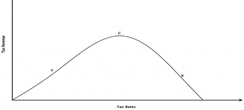
As can be seen in Figure 1, as tax rates increase, tax revenues rise to point (y), reach a peak labelled point (c) and begin to fall to point (x), up to the extent where zero-revenues are realised. Laffer (1921) reasoned that higher tax rates discourage work, output and investment and in extreme cases, induce tax avoidance and evasion. In other words, unreasonably high tax rates could be the cause of low growth rates in certain countries. Interestingly, changes in tax rates appear to have two effects: the arithmetic effect and the economy effect. The arithmetic effect entails situations in which tax rate cuts result in declines in tax revenues (per dollar of the tax base) by an amount equal to the tax cut. The economy effect on the one hand, refers to situations in which lower tax rates encourage participation in taxed economic activities such as work, employment and output. Given these explanations, one can tell that the arithmetic effect and economy effect work in opposite directions. Having said that, the conclusion as to whether tax cuts result in increased tax revenues depends on the extent that the economy effect outweighs the arithmetic effect.

Although different taxes are levied on different sources of revenue, what matters ultimately is not necessarily the impact of each tax in isolation, but the overall impact of the tax-mix on the welfare of individuals (Creedy, 2009). Notably, there is no clear and direct connection between taxes paid by an individual and the provision of public goods and services to the individual taxpayer. This is because; individuals are obliged to pay taxes by law even if there are no direct benefits in return. Economists regard the best tax systems as those characterised by broad tax bases and low tax rates (Matthews, 2011). The reasoning behind this is that the tax burden is much greater when a small pool of individuals is taxed at higher rates than when a large pool of individuals is taxed at lower rates.

2.2. Empirical literature

This subsection covers empirical studies that have investigated the determinants of tax capacity and tax effort thereof. It is sufficient to note on the onset, that the majority of studies conducted on tax capacity and effort are panel studies. As mentioned earlier, country-specific studies are a recent phenomenon. Thus, the majority of studies covered in this subsection are panel studies.

Brafu-Insaidoo & Obeng (2019) investigated the determinants of tax capacity and tax effort in Ghana by linking Ghana’s revenue-generating potential with desired expenditure needs. The study employed the stochastic frontier model on time series data spanning from 1985 to 2014. The key finding was that institutional quality and tax base expansions contributed significantly to Ghana’s revenue-generating potential during the period under study. In addition, the authors found that reductions in political instability and corruption level benefited administrative efficiency in the tax system.

Murunga et al. (2016) examined the drivers of domestic revenue mobilisation in Kenya for the period 1980–2015. The study utilised the Ordinary Least Squares econometric technique to analyse macroeconomic data ranging from 1980 to 2015. Based on findings, per capita GDP, share of agriculture in GDP and share of service sector in GDP have a positive and statistically significant impact on domestic revenue mobilisation. In addition, the findings revealed that Kenya’s tax effort was below unity during the period under consideration. This implies that Kenya’s tax effort falls short of its tax capacity.

Khwaja & Iyer (2014) estimated the determinants of revenue-generating potential in 61 countries. They adopted a dual approach to revenue potential: one based on the economic structure and strength of a country and the other based on the legislation. Their study revealed that the revenue potential in legal terms is much higher than the revenue potential in economic terms for most Eastern Europe and Central Asia countries. In addition, they found that the tax gap is higher when the underground economy is considered, implying that countries with a greater share of the underground economy collect way less in tax revenue than they could, given their economic strength.

Attiya & Umaima (2012) investigated the factors contributing to the revenue-generating potential in a sample of developing Asian countries over the period 1984–2010. The results showed that both GDP per capita, foreign debt and share of agriculture in GDP are statistically significant in explaining variations in revenue performance. In addition, institutional factors, good governance, control for corruption and trade openness are also found to have a positive and statistically significant impact on revenue potential. Notwithstanding, their tax effort results indicated that countries which are heavily dependent on the agricultural sector tend to have poorer revenue performance.

Davoodi & Grigorian (2007) seek to identify a proximate set of factors that contribute to Armenia’s stubbornly low tax-to-GDP ratio using panel data spanning from 1990 to 2004 in 141 countries. They utilised several econometrics techniques including fixed effects, random effects and OLS. Their findings indicate that Armenia’s tax effort falls short of its potential by as much as 6½ percent of GDP and this is largely due to weak institutions and a larger shadow economy.

Le et al. (2012) undertook a unique study by providing four classifications of tax: high collection, low collection, high effort and low effort. They utilise Panel OLS on cross-country data spanning from 1994 to 2009 in 110 developing and developed countries. Like many other studies, they find that nations with better institutional quality have the potential to collect higher tax revenues. Even more, they find that developing nations have more limitations to expand the scope for taxation, efficiently and equitably.

Gupta (2007) undertook a study aimed at estimating the principal determinants of tax revenue potential using a sample of 105 developing countries. The study runs from 1980 to 2004 utilising two commonly used econometric techniques of fixed effects and random effects. Based on findings, several structural factors including GDP per capita, Trade openness and foreign aid are found to be statistically significant and positively correlated with higher tax revenues. On the contrary, agricultural share in GDP is found to be statistically significantly but negatively associated with revenue performance. Furthermore, the study reveals that countries that rely heavily on taxes on goods and services collect lower tax revenues.

Mertens (2006) estimated tax capacity and tax effort for ten Central and Eastern Europe countries using panel data spanning from 1992–2000. Unlike other studies, agriculture’s share of GDP was used as a proxy for the level of economic development while industry and import sector share of GDP were used as proxies for tax handles. Nonetheless, the results of the study indicate that both the level of development and sectoral shares of GDP are significant determinants of tax capacity. In addition, the tax effort index ranges between 0.809 and 1.257.

3. Empirical strategy

This section unpacks the methodology of the study, including the type and sources of data used. Furthermore, the section details variables included in the model as well as various econometrics techniques utilised.

3.1. Model specification

The model of this study is built on the demographic, economic, policy and institutional factors of the country. This is in line with existing empirical studies (i.e. Attiya & Umaima, 2012; Karagöz, 2013; Khwaja & Iyer, 2014; Ananou & Houngbonon, 2015; Jalles, 2017). Trotman-Dickenson (1996) defines taxable capacity as the ability of businesses and individuals to pay taxes.

3.1.1. A measure of tax capacity

The model is expressed as follows: (1) $\left(\frac{T}{Y_t}\right)=\mu +\text{β}.X_t+\mathrm{\partial }+{ϵ}_t$(1) where $\left({{\displaystyle \frac{T}{Y}}}_t\right)$ is the tax-GDP ratio, $\mu$ is a constant, $\text{β}$ is the slope coefficients of the parameters, $\mathrm{\partial }$ is a dummy for the 2008 crisis, ${ϵ}_t$ is the idiosyncratic error term with usual properties $\sim N\left(0,{\sigma }^2\right)$ and $X_t$ is the vector consisting of control variables that affect tax revenue: (2) $\begin{array}{rl}{X}_t=& (GDP{C}_t+TO{P}_t+AG{R}_t+MA{N}_t+SER{V}_t+GO{V}_t+PO{P}_t+IN{F}_t\\ & +EMP{L}_t+LFP{R}_t+CO{R}_t)\end{array}$(2) in which case $GDPC$ is GDP Per Capita (constant 2010 prices) measuring the level of household incomes, $TOP$ is trade openness measured by trade-GDP ratio, $AGR$ is the share of agriculture in GDP, $MAN$ is the share of manufacturing in GDP, $GOV$ is the Polity IV index used as a proxy for good governance, $INF$ is the inflation rate measured by the Consumer Price Index (CPI), $SER{V}_t$ is services share in GDP, $EMPL$ is the employment to population ratio, $LFPR$ is the labour force participation rate,$POP$ is population growth and $COR$ is corruption measured by the corruption score index. Most empirical studies (Davoodi & Grigorian, 2007; Attiya & Umaima, 2012; Khwaja & Iyer, 2014) have utilised Fixed Effects (FE), Random Effects (RE), Generalised Method of Moments (GMM) and Panel OLS techniques. In our case, we employ the Instrumental Variable (IV) technique, 2Stage Least Squares (2SLS) to be specific, given the threat of endogeneity in our model.

3.1.2. A measure of tax effort

Tax effort is the extent to which taxable capacity is being used. This can be obtained from the ratio between actual tax capacity and potential tax capacity. Following (Davoodi & Grigorian, 2007; Attiya & Umaima, 2012; Khwaja & Iyer, 2014), our simple calculation of tax effort index is expressed as: (3) $TE=\frac{\left(T/Y\right)}{\left(\hat{T}/Y\right)}$(3) where $\left({\displaystyle \frac{T}{Y}}\right)$ is the actual tax capacity and $\left({\displaystyle \frac{\hat{T}}{Y}}\right)$ is the potential tax capacity. The potential tax capacity was estimated using Equation (1). The values of tax effort should be between zero and one. A tax effort index that lies below the regression line implies that the country falls short of its potential tax capacity whereas a tax effort index above the regression line indicates that a country performs well above its potential tax capacity.

3.2. Data description

The study made use of annual secondary time series data spanning from 1960–2017. The data was collected from numerous secondary servers including World Development Indicators (WDI), South African Reserve Bank (SARB), South African Revenue Services (SARS), PolityIV, Federal Reserve Economic Data (FRED), Transparency International and National Treasury of South Africa.

3.3. Justification of variables

GDP per capita measures a household income levels and is expected to be positively associated with the government’s ability to collect taxes. As income levels rise, tax revenues would follow suit due to automatic stabilisers. The relationship between trade openness and revenue mobilisation is twofold. On the one hand, economies that are extremely open to trade are likely to collect fewer tax revenues on imports as trade taxes are relatively low (Gupta, 2007). On the other hand, open economies are known to grow faster, hence higher levels of GDP, consequently higher revenue collections. The inclusion of the agriculture sector is very crucial as it represents difficulties incurred by official in collecting taxes.

Governments usually offer tax exemptions and subsidies to farmers and this reduces the size of the tax base. Thus, the sign for agriculture is expected to be negative. The growing body of literature has highlighted the importance of good governance and quality institutions in tax collections. These factors affect tax collections through their contributions to tax evasion, weak administration and improper tax exemptions (Davoodi & Grigorian, 2007). The sign for good governance is expected to be positive. Le et al. (2012) notes that population growth distorts tax collection capacity and lower the fraction of productive population. This is true if dependency population is greater than working age population or the labour force. Hence, population growth is expected to have a negative sign.

Like trade openness, the impact of inflation on revenue collection remains ambiguous. While Musharraf et al. (2013) state that inflation may increase revenues in progressive tax systems, Attiya & Umaima (2012) argue that inflation has a negative impact on revenue mobilisation through the consumption and investment channels. Since South Africa is faced by a progressive tax system, inflation is expected to have a positive sign. The corruption perception index ranks countries based on how corrupt the country’s public sector is perceived to be by experts and business executives (Transparency International, 2012). The lower the score, the more corrupt the country is perceived to be and vice versa. This variable is expected to have a positive impact on revenue mobilisation as low levels of corruption improve tax administration efficiency. Both the labour force participation rate and employment–population ratio are expected to have positive signs. The reasoning is that, higher employment levels result in increased economic activity and thus income generation, which is then taxed and collected by tax authorities.

3.3. Estimation techniques

3.3.1. Unit root tests

One of the basic principles of econometric modelling is testing for stationarity of variables, more especially when dealing with time series data (Arltova & Fedorova, 2016). The reasoning is that non-stationary variables may lead to spurious results or even break the model. Thus, to avoid this, we began by testing the variables for unit root using Augmented Dickey Fuller (ADF) (Dickey & Fuller, 1979) and Phillips–Perron (PP) (Phillips & Perron, 1988) non-stationarity tests. The choice of techniques was based on their simplicity, since there is no uniformly better test for unit root.

3.3.2. 2Stage Least Squares

As stated earlier in the study, we employed the IV technique given the threat of endogeneity in our model. Consider a simple regression equation: (7) $y=\mu +\delta x+ϵ$(7) where $y$ is the dependent variable, $\mu$ is the constant, $\delta$ is a slope parameter to be estimated, $x$ is the independent variable and $ϵ$ is the error term. If $x$ and $ϵ$ are correlated, then this violates an assumption of the regression framework (Oczkowski & Farrell, 1998). Notably, if we apply the standard OLS technique, the coefficients will be biased and inconsistent. To remedy this, one can apply the instrumental variable technique. The instruments (say $v$) however, should satisfy two conditions: (i) $v$ should be uncorrelated with $ϵ$, and (ii) $v$ must be correlated with $x$. An advantage of the technique is that it easily caters for non-linear and interactions effects (Bollen & Paxton, 1998). Even more, it produces consistent results even when $x$ and $ϵ$ are correlated. The procedure involves two stages of OLS:

• - An OLS regression$x$ on $v$ and get predictions for $x$, say $\hat{x}$.

• - OLS regression $y$ on $\hat{x}$.

3.3.3. Residual diagnostics

Time series analysis is not without risk and chief among those risks are the risks of heteroscedasticity and serial correlation. Thus, to ensure that our models do not suffer from serial correlation and heteroskedasticity, we ran several diagnostic tests ranging from Breusch–Godfrey Serial Correlation LM test (Breusch 1978; Godfrey, 1978), White-Heteroscedasticity test (White, 1980), Jarque-Bera Normality test and CUSUM stability tests. The CUSUM test was used to determine the stability of the model.

4. Findings and discussions

This section details findings from econometric tests performed. These include stationarity tests, regression output, residual diagnostics and calculations for tax effort.

4.1. Descriptive statistics

We begin by presenting the descriptive statistics of individual variables to assess their mean and standard deviations. Table 1 details the minimum, maximum, standard deviation and mean value for each variable. Tax revenue has a mean of 20.7 and standard deviation of 3.36 while the labour force participation rate has the highest average, amounting to 53.5, followed by services share in GDP (53.4), trade openness (52.1) and corruption index (46.8). Standard deviation measures the spread of the data distribution. The more spread out a data distribution is, the greater its standard deviation and the less spread out a data distribution is, the smaller its standard deviation. It is worth noting that a standard deviation doesn’t tell us much about the quality of the data.

Table 1. Descriptive statistics.

	Mean	S-Deviation	Min	Max	Obs.
Tax Revenue %GDP	20.77	3.37	13.90	25.70	58
Trade Openness	52.13	7.15	37.49	72.86	58
GDP Per capita	4.67	0.05	4.53	4.75	58
Agriculture %GDP	5.14	2.60	2.08	11.01	58
Governance	6.14	2.44	4.00	9.00	58
Population growth	2.08	0.61	1.05	2.79	58
Inflation	8.06	4.93	−1.63	18.52	58
Manufacturing %GDP	18.57	3.34	11.61	22.61	58
Services %GDP	53.41	5.66	43.07	61.49	58
Corruption Index	46.79	3.78	41.00	56.80	22
Employment ratio	40.89	1.53	38.52	44.31	27
Labour force rate	53.50	0.77	52.31	55.78	28

Source: author’s computations.

Trade openness has the highest standard deviation of 7.15, indicating that the values are spread out. On the contrary, GDP per capita, labour force participation rate and population growth have low standard deviations of 0.05, 0.77 and 0.6, respectively. This shows that most of the data points are very close to the mean. Governance on the one hand, has a mean of 6.14 and standard deviation of 2.44, insinuating that the data points are slightly close to the mean. We do note that the employment ratio and labour force participation rate have fewer observations and might not yield credible results. Thus, they will serve as redefined proxy of population growth.

4.2. Pairwise correlation

Table 2 details correlations amongst the variables in question. Correlation estimates provide a useful tool for analysing and understanding the relationship between the dependent variable and independent variables, identifying and confirming the expected signs of variables as well as detecting issues of multicollinearity. From Table 2, it is evident that most of the independent variables are highly correlated, implying that the model is most likely to suffer from multicollinearity. Nonetheless, trade openness and inflation are found to be weakly and positively correlated with tax revenue. On the contrary, population growth and agriculture share in GDP are found to be strongly and negatively correlated with tax revenue. These findings are in line with Le et al. (2012) and Gupta (2007). Governance and GDP per capita are found to be strongly and positively associated with tax revenue. The presence of good governance enables tax authorities to collect and administer tax revenue more efficiently.

Table 2. Pairwise correlation test results.

	REV	TOP	POPG	GOV	GDPP	AGR	INF	SERV	MAN	EMPL	LFPR	COR
REV	1.00
TOP	0.35 0.00*	1.00 –
POPG	−0.84 0.00*	−0.50 0.00*	1.00 –
GOV	0.74 0.01*	0.36 0.00*	−0.91 0.00*	1.00 –
GDPP	0.77 0.00*	0.56 0.00*	−0.60 0.00*	0.48 0.04**	1.00 –
AGR	−0.95 0.00*	−0.25 0.05*	0.82 0.00*	−0.78 0.00*	−0.76 0.00*	1.00 –
INF	0.23 0.00*	−0.08 0.02**	0.24 0.00*	−0.35 0.00*	0.23 0.00*	−0.14 0.00*	1.00 –
SERV	0.69 0.00*	0.30 0.00*	−0.89 0.00*	0.94 0.00*	0.49 0.00*	−0.75 0.00*	−0.45 0.00*	1.00 –
MAN	−0.68 0.00*	−0.62 0.00*	0.86 0.00*	−0.82 0.00*	−0.64 0.00	0.67 0.00*	0.36 0.01**	−0.86 0.00*	1.00 –
EMPL	0.40 0.31	0.28 0.06***	−0.18 0.00	−0.45 0.01*	0.16 0.13*	0.03 0.02**	0.28 0.01*	−0.15 0.00*	−0.01 0.02**	1.00 –
LFPR	0.81 0.00*	0.65 0.00*	−0.51 0.02**	0.16 0.38	0.65 0.00*	−0.48 0.00*	0.13 0.85	0.42 0.06***	−0.55 0.00	0.54 0.03**	1.00 –
COR	−0.32 0.14	−0.45 0.04**	0.46 0.03**	NA	−0.69 0.00*	0.81 0.00*	0.44 0.04**	−0.85 0.00	0.73 0.00	0.44 0.04**	−0.19 0.41	1.00 –

Notes: TOP – trade openness; POPG – population growth; GOV – Good governance; REV – tax revenue/GDP; GDPP – GDP per capita; LFPR – labour force participation rate; AGR – agriculture/GDP; EMPL – employment/population ratio; MAN – manufacturing/GDP; SERV – services/GDP; COR – corruption score index; INF – Inflation rate. *, **, *** indicate significance at 1%, 5% and 10%, respectively

Agriculture share of GDP, manufacturing share of GDP, services share of GDP and industry share of GDP are perfectly correlated with population growth, amounting to (in absolute terms) 82%, 89%, 86% and 87%, respectively. Even worse, we find a strong correlation between governance, services share in GDP, manufacturing share in GDP and industry share in GDP, measuring 93%, 82% and 91%, respectively.

4.3. Stationarity analysis

As noted earlier on, we used both ADF and PP stationarity tests. It is sufficient to note that the PP test has more power over the ADF test. Thus, in cases where one or more variables is/are inconsistent across tests, the conclusion will be based on the PP test. Table 3 shows the results from the stationarity tests. From the stationarity tests performed, we find that tax revenue, economic development, governance, population growth, manufacturing and services share in GDP, employment–population ratio and trade openness are consistent in all tests and stationary after 1st differencing.

Table 3. Stationarity tests results.

Variable	Augmented Dicker Fuller test			Phillip–Perron test
	Intercept	Trend and intercept	Order of integration	Intercept	Trend and intercept	Order of integration
REV	−1.36	−2.86		−1.32	−2.80
D(REV)	−7.52*	−7.52*	| (1)	−8.73*	−10.08*	| (1)
GDPC	−2.39	−2.56		−2.24	−2.20
D(GDPC)	−4.52*	−4.59*	| (1)	−4.56*	−4.63*	| (1)
TOP	−2.17	−2.57		−2.08	−2.48
D(TOP)	−7.36*	−7.29	| (1)	−8.22*	−8.51*	| (1)
GOV	−0.65	−1.91		−0.64	−1.91
D(GOV)	−7.55*	−7.49*	| (1)	−7.55*	−7.49*	| (1)
INF	−1.98	−2.01		−2.98**	−2.95	| (0)
D(INF)	−12.03*	−7.10*	| (1)	–	–
POPG	−0.19	−2.39		−0.33	−2.32
D(POPG)	−3.30**	−3.49**	| (1)	−2.93**	−2.93	| (1)
AGR	−3.57*	−1.63	| (0)	−3.66*	−2.33	| (0)
MAN	0.57	−2.12		0.514	−2.07
D(MAN)	−6.50*	−6.20*	| (1)	−6.47*	−7.07*	| (1)
SERV	−0.59	−1.91		−0.35	−1.55
D(SERV)	−5.48*	−5.46*	| (1)	−5.32*	−5.28*	| (1)
COR	−3.10**	−3.87**	| (0)	−3.09**	−3.79**	| (0)
LFPR	−2.97**	−3.17	| (0)	−1.95	−2.17
D(LFPR)	-	-		−4.00*	−3.94**	| (1)
EMPL	−2.41	−2.56		−1.96	−2.21
D(EMPL)	−4.19*	−4.11*	| (1)	−4.18*	−4.09*	| (1)
Critical values				Critical values
1%	−3.55	−4.12		−3.55	−4.13
5%	−2.91	−3.49		−2.91	−3.49
10%	−2.59	−3.17		−2.59	−3.17

*, **, *** indicate significance at 1%, 5% and 10%, respectively.

In addition, corruption index and agriculture share in GDP are also found to be consistent across all tests yet stationary at level. Only inflation and the labour force participation rate are found to be inconsistent across both tests. The conclusion is based on the PP test given its power over ADF. Hence, inflation is stationary at level whereas the labour force participation rate is stationary after 1st differencing. Interestingly, no variable is found to contain a trend.

4.4. Regression outputs

The main regression output is provided in Table 4. The total number of observations is 58 and the value of R-squared is significant (95%), implying that the model fits the data well. The Durbin-Watson value of 1.74 is near 2, insinuating that the model is less likely to suffer from serial correlation. As stated earlier in the study, we made use of 2SLS econometric technique to accommodate the risk of endogeneity. Trade openness to begin with, has a negative and statistically significant impact on tax capacity. The economic intuition is that South Africa is an open economy and thus collects less tax revenues from trade since trade taxes and barriers are relatively low. On the contrary, household incomes are found to have a huge positive and statistically significant impact on tax capacity. This is consistent with existing literature (i.e. Piancastelli, 2001; Davoodi & Grigorian, 2007; Gupta, 2007; Garg et al., 2017).

Table 4. Regression output.

Dependent variable: Tax-GDP Ratio
Variable	TOP	POPG	GOV	GDPP	AGR	INF	MAN	SERV	DUM	C
Coefficient	−3.51	−4.31	1.26	9.22	−2.77	0.23	−3.05	−4.58	−0.89	21.91
S.E	(1.91)***	(1.20)*	(1.02)	(5.15)***	(0.96)*	(0.04)*	(2.51)	(4.71)	(0.74)	29.61
T-stat	−1.84	−3.59	1.23	1.79	−2.88	6.02	−1.22	−0.97	−1.20	0.74

Notes: TOP – trade openness; POPG – population growth; GOV – Good governance; GDPP – GDP per capita; INF – Inflation rate; AGR – agriculture/GDP; MAN – manufacturing/GDP; SERV – services/GDP. $R^2$(0.95), DW-stat (1.74), IV tank (9). *, **, *** indicate significance at 1%, 5% and 10%, respectively.

The substantial value for GDP per capita is not surprising since personal and corporate income taxes make-up a larger fraction of tax revenues in South Africa. Good governance is found to have a weak positive and statistically insignificant impact on tax capacity whereas population growth has a strong negative and statistically significant impact on tax capacity. Bird et al. (2004) and Attiya & Umaima (2012) also found an inverse relationship between population growth and revenue mobilisation. A unit increase in population growth decreases tax capacity by as much as 4.3 units. The reasoning is that, as the population increases, the tax base becomes more complex, making it difficult for the government to identify and tax potential candidates. Even worse, a less educated population is most likely to dependent heavily on the government to make ends meet, usually through social grants. Agriculture has a negative sign as expected and is significant in explaining variations in tax capacity.

Inflation on the contrary, has a positive sign, which is expected in a country following a progressive tax system. A unit increase in inflation can increase tax capacity by approximately 0.23 units whereas a unit increase in agriculture decreases revenue collections by approximately 2.8 units (in line with Karagöz, 2013; Garg et al., 2017). The negative impact of agriculture on revenue collections is not surprising, as the government issues subsidies for agricultural production. Also, it seems politically infeasible to tax the agricultural sector as this might discourage production and hamper food security. Moreover, given the low prices and profits in the agricultural sector, the government would collect little revenue, that is to say, the costs of taxing the agricultural sector would outweigh the benefits. Manufacturing and industry share in GDP are found to have a strong negative impact on revenue mobilisation though statistically insignificant in explaining variations in revenue mobilisation.

4.5. Residual diagnostics

To ensure that the model is valid, we ran residuals tests. Performing residual diagnostics has become a requirement in econometric analysis. Figure 2 displays the output from the Jarque-Bera normality test. From Figure 2, we can see that the kurtosis is 2.80, which is approaching the recommended value of 3.7.

Figure 2. Normality test results.

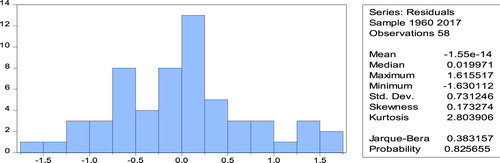
The corresponding Jarque-Bera p-value is 83%, greater than 5% and indicating that the data is normally distributed. We performed further residual diagnostics, presented in Table 5.

Table 5. Residual tests results.

Serial correlation (Breusch–Godfrey)		Heteroscedasticity (Breusch–Pagan–Godfrey)		Heteroscedasticity (Harvey)
Obs.*R	Prob. Chi (1)	Obs.*R	Prob. Chi-	Obs.*R	Prob. Chi
1.13	0.29	16.37	0.06	10.90	0.28

Source: author’s computations.

As can be seen in Table 5, the model does not suffer from serial correlation nor heteroscedasticity. This is because; the corresponding p-values are greater than 5%, which leads to a rejection of the null hypothesis. The corresponding p-values for both serial correlation and heteroscedasticity are 29% and 28%, respectively. Lastly, we performed residual stability tests to ensure that the model is stable. We followed the OLS approach to achieve this goal, presented in Figure 3.

Figure 3. OLS CUSUM stability test results.

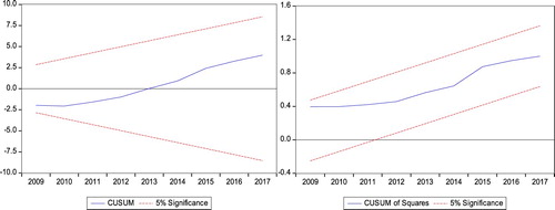
It is unquestionably clear from Figure 3 that the model is stable overtime. Both the CUSUM and CUSUM of squares tests confirm this. Given these residual diagnostics, we can confidently confirm that the model is indeed valid.

4.6. Robustness tests

To ensure that the results in Table 4 are robust, we ran alternative specifications. The results are presented in Table 6. Robustness checks are usually conducted to ensure that the initial model is consistent and robust. To achieve this, we introduced three control variables to our initial model, that is: labour force participation rate, employment–population ratio and corruption index.

Table 6. Robustness tests results.

Dependent variable: Tax-GDP ratio
	Model (1)	Model (2)	Model (3)	Model (4)
C	3.33	−1.21	−13.01	11.50
TOP	−2.40 (1.53)	−1.79 (1.36)	1.93 (2.03)
POPG	−3.91 (1.12)*	−3.93 (1.12)*	–	−2.25 (0.95)**
GOV	0.66 (0.82)	0.76 (0.80)	–	0.29 (1.07)
GDPP	7.89 (4.96)	7.18 (4.88)	–	–
INF	0.24 (0.03)*	0.23 (0.03)*	0.01 (0.06)	0.10 (0.05)**
AGR	−2.90 (0.95)*	−3.22 (0.88)*	−0.57 (2.45)
MAN	−2.00 (2.27)	–	−6.93 (3.59)***	−8.30 (2.24)*
SERV	–	–		–
DUM	−0.79 (0.73)	−0.28 (0.46)	−1.58 (0.73)**	−1.45 (0.75)***
COR	–	–	3.90 (3.49)	–
LFPR	–	–	0.60 (0.17)*	–
EMPL	–	–	–	9.39 (4.68)***
Adj.$R^2$	0.94	0.94	0.84	0.75
F-stat	121.10	138.90	14.85	14.10
DW-stat	1.78	1.67	1.89	1.88
No of Obs.	58	58	22	27
Tank	9	8	8	7

*, **, *** indicate significance at 1%, 5% and 10%, respectively. Technique used is 2SLS (Robust S.E are in parenthesis).

In model (1) and (2), we omit both manufacturing and services share in GDP. The results remain consistent, yet trade openness becomes insignificant. In model (3), we replace GDP per capita, population growth and governance with labour force participation rate and corruption index, respectively. Inflation becomes negative whereas trade openness becomes positive, albeit statistically insignificant. The corruption index is found to have a strong positive impact on revenue mobilisation though statistically insignificant. The effects of the labour force participation rate on revenue mobilisation are found to be weakly positive and statistically significant. This shows that the government could collect higher tax revenues from personal and corporate income taxes through increased labour participation in the economy. In addition, given that South Africa has made huge investments in human capital through the fee-free higher education system, such human capital can benefit the country in the form of increased tax revenues in the long run. However, this can happen only and only if sufficient jobs are created in the labour market to absorb existing inventories in human capital.

In model (4), we replace the labour force participation rate with employment–population ratio. We find that employment–population ratio has a strong positive and statistically significant impact on revenue mobilisation. Furthermore, the impact of employment–population ratio on revenue mobilisation is relatively greater and statistically significant than that of the labour force participation rate. These findings imply that the employment–population ratio is better at explaining variations in revenue mobilisations than the labour force participation rate, at least in this study. We can observe from Table 6 that our initial estimates in Table 4 are consistent and robust. This stems from the fact that the values and signs of coefficients in Table 6 are not altered significantly when adding or deducting control variables.

4.7. Tax effort indices

Table 7 shows the tax effort index calculated from the 2SLS estimates in Table 4. The shaded cells indicate periods in which tax effort indices were equal to and above one. That is to say, they signal periods in which South Africa performed well above its potential tax capacity while the unshaded cells indicate periods in which South Africa fell short of its potential capacity. As can be seen in Table 7, the highest tax effort index was 1.10 in 1963 before hitting a record low of 0.92 in 2002. Interestingly, on average, the tax effort index is 1.00, implying that actual tax capacity equals potential tax capacity. It is also evident that, in most periods, South Africa performed well above its potential tax capacity. This is indicated by the values above and equal to 1. As indicated in Table 4, the driving forces behind South Africa’s tax capacity are GDP per capita, agriculture share in GDP, population growth, inflation and trade openness. This is consistent with Teera & Hudson (2004) as they found that upper middle-income and high-income OECD countries are making better use of their tax bases to increase revenue.

Table 7. Tax effort index results for South Africa.

Date	Actual tax capacity	Potential tax capacity	Tax effort	GDP per capita
1960	14.6	14.26	1.02	316
1961	13.9	14.47	0.96	324
1962	13.9	14.58	0.95	336
1963	15.7	14.40	1.09	363
1964	15.3	15.57	0.98	388
1965	15.6	15.46	1.01	413
1966	15.4	15.85	0.97	438
1967	16.1	15.39	1.05	475
1968	15.9	16.00	0.99	500
1969	15.9	16.61	0.96	548
1970	16.2	17.25	0.94	585
1971	17	17.53	0.97	631
1972	17.5	17.55	1.00	695
1973	18.5	18.26	1.01	841
1974	18.7	18.85	0.99	1011
1975	18.7	18.54	1.01	1113
1976	19.5	18.71	1.04	1229
1977	19.4	19.01	1.02	1333
1978	19.5	19.29	1.01	1495
1979	20	20.36	0.98	1745
1980	20	20.76	0.96	2271
1981	19.6	19.96	0.98	2575
1982	20.3	20.46	0.99	2857
1983	20.2	20.82	0.97	3193
1984	20.3	21.19	0.96	3658
1985	22.3	22.18	1.01	4129
1986	22.3	22.51	0.99	4734
1987	21.5	21.49	1.00	5416
1988	22.3	21.00	1.06	6363
1989	23.5	21.97	1.07	7479
1990	24	22.38	1.07	8430
1991	22.2	22.76	0.98	9451
1992	21.2	21.30	1.00	10 377
1993	21	21.02	1.00	11 623
1994	21.8	21.71	1.00	12 870
1995	21.6	21.56	1.00	14 320
1996	22.4	22.15	1.01	15 782
1997	22.3	21.92	1.02	17 122
1998	23.3	22.91	1.02	18 162
1999	23.4	22.03	1.06	19 493
2000	22	23.19	0.95	21 657
2001	23.4	22.43	1.04	23 481
2002	22.6	24.23	0.93	26 778
2003	21.8	21.77	1.00	28 632
2004	22.3	23.36	0.95	31 370
2005	24.1	24.07	1.00	34 281
2006	25.2	25.03	1.01	37 899
2007	25.5	25.59	1.00	42 863
2008	25.5	24.58	1.04	47 512
2009	23.2	24.67	0.94	49 682
2010	23.3	24.19	0.96	53 823
2011	24	24.73	0.97	58 559
2012	23.9	24.47	0.98	62 297
2013	24.3	24.23	1.00	66 952
2014	24.4	24.09	1.01	71 064
2015	25.6	24.50	1.04	74 663
2016	25.7	25.05	1.03	79 066
2017	25.3	24.68	1.02	83 393
Average	20.77	20.77	1.00	18 776.83

4.7.1. Trends in tax effort and major economic events

Figure 4 shows trends in tax effort for South Africa. It is apparent in Figure 4 that the tax effort index is time variant. This may be attributable to major political and economic events that took place over the estimation period.

Figure 4. Trends in tax effort for South Africa. Source: Author’s computations.

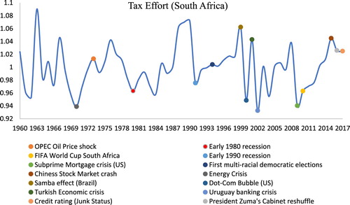
Global economic events such as the energy crisis and Chinese stock market crash often have spill-over effects which have downstream impact on tax performance for South Africa. For example, the 2008 subprime crisis left majority of economies in bad economic shape, following declines in output, high unemployment rates, consequently, declines in income levels. Considering that a major component of tax revenue is income tax, a decline in income levels would reduce tax revenues by a significant amount, thus undermining tax effort. The tax effort index gained momentum in early 2010 amid the FIFA World Cup hosted by South Africa. Following this, the tax effort index took a knock in the late 2016 following a combination of major political decisions and economic events, to name a few, the cabinet reshuffle and downgrade of the country’s investment status by Rating Agencies.

5. Conclusion and evaluation

This study was aimed at investigating the determinants of tax capacity and calculating tax effort for South Africa. The findings revealed that South Africa’s tax effort has been above unity for most of the period under study. In addition, we found that on average, the tax effort index is 1, implying that actual tax capacity matches potential tax capacity. Furthermore, the regressions performed were found to be robust and free from potential risks of serial correlation and heteroscedasticity. Based on 2SLS findings, the determinants of tax capacity for South Africa are GDP per capita, agriculture share in GDP, trade openness, inflation and population growth.

5.1. Policy insights evaluation

Given that household incomes and population growth were found to be major determinants of tax capacity in South Africa, adequate investments in human capital and job creation need to take place for the government to generate value from its rapidly growing population. Also, tax rates have been hiked numerous times in South Africa. Raising the tax rates any further might discourage economic activity in the form of labour, output and investment. Even worse, higher tax rates often induce tax avoidance and evasion, creating about their own problems than solutions. Thus, an optimal solution to raising tax revenues is broadening the tax base, thereby lowering tax rates in the long run. Fortunately, as stated earlier, South Africa is abundant in human capital, and if such human capital is to be absorbed by the labour market, the tax base would expand to an appreciable extent, yielding sufficient revenues for government to meet its desired expenditure needs.

Acknowledgements

The financial assistance of the National Treasury towards this research is hereby acknowledged. Opinions expressed, and conclusions arrived at are those of the authors and should not be attributed to the National Treasury.

Disclosure statement

No potential conflict of interest was reported by the author(s).

References

- Ade, M, Rossouw, J & Gwatidzo, T, 2018. Determinants of tax revenue performance in the Southern African Development Community. ERSA working paper no.762.
- Agarwal, P, 2018. The Laffer curve. https://www.intelligenteconomist.com/laffer-curve/.
- Ananou, F & Houngbonon, GV, 2015. Exploring the dynamic of the tax gap in Africa. Paris School of Economics & Orange, Paris.
- Arltova, M & Fedorova, D, 2016. Selection of unit root test on the basis of length of the time series and value of AR (1) parameter. Journal of Statistika 96(3), 47–64.
- Attiya, J & Umaima, A, 2012. Analysis of revenue potential and revenue effort in developing Asian countries. The Pakistan Development Review 51(4), 365–80.
- Bird, RM, Martinez-Vazquez, J & Torgler, B, 2004. Societal institutions and tax efforts in developing countries. Andrew Young School of Policy Studies, Georgia State University, Georgia (working paper 04-06).
- Bollen, KA & Paxton, P, 1998. Interactions of latent variables in structural equation models. Structural Equation Modelling 5, 267–93.
- Brafu-Insaidoo, WG & Obeng, CK, 2019. Estimating Ghana's tax capacity and effort. African Economic Research Consortium policy brief no.682.
- Breusch, TS, 1978. Testing for autocorrelation in dynamic linear models. Australian economic papers.
- Cohen, MC, 1983. Tax capacity, tax effort, and state funding of schools in Ohio. Journal of Education Finance 4(9), 141–56.
- Creedy, J, 2009. The personal income tax structure: Theory and policy. Department of Economics, working papers series 1063. University of Melbourne.
- Davoodi, HR & Grigorian, DA, 2007. Tax potential vs. tax effort: A cross-country analysis of Armenia’s stubbornly low tax collection. IMF Working Paper, No. 07/106.
- Dickey, DA & Fuller, WA, 1979. Distribution of the estimators for autoregressive time series with a unit root. Journal of the American Statistical Association 74, 427–31.
- Garg, S, Goyal, A & Pal, R, 2017. Why tax effort falls short of tax capacity in Indian states: A stochastic frontier approach. Public Finance Review 45(2), 232–59.
- Godfrey, LG, 1978. Testing against general autoregressive and moving average error models when the regressors include lagged dependent variables. Econometrica 46, 1293–301.
- Gupta, AS, 2007. Determinants of tax revenue efforts in developing countries. IMF working paper no.7/184.
- Jalles, JT, 2017. Tax buoyancy in sub-Saharan Africa: An empirical exploration. African Development Review 29(1), 1–33.
- Karagöz, K, 2013. Determinants of tax revenue: does sectorial composition matter? Journal of Finance, Accounting and Management 4(20), 50–63.
- Khwaja, MS & Iyer, I, 2014. Revenue potential, tax space, and tax gap. A comparative analysis. Policy Research working paper. World Bank.
- Le, TM, Moreno-Dodson, B & Bayraktar, M, 2012. Tax capacity and tax effort extended cross-country analysis from 1994 to 2009. Policy Research working paper 6252, World Bank.
- Leuvennink, J, 2017. Tax revolt may be brewing in South Africa. Fin24 News. https://www.fin24.com/Budget/Budget-and-Economy/tax-revolt-may-be-brewing-in-south-africa-20171025.
- Lotz, JR & Morss, ER, 1967. Measuring “tax effort” in developing countries. Staff Papers (International Monetary Fund) 14(3), 478–99.
- Matthews, S, 2011. What is a competitive tax system? OECD taxation working papers, no. 2, OECD Publishing.
- Mertens, JB, 2006. Measuring tax effort in Central and Eastern Europe. Journal of Public Finance and Management 3(4), 530–63.
- Mitchell, DJ, 2012. The Laffer curve shows that tax increases are a very bad idea. Forbes Online News. https://www.forbes.com/sites/danielmitchell/2012/04/15/the-laffer-curve-shows-that-tax-increases-are-a-very-bad-idea-even-if-they-generate-more-tax-revenue/#47daada87e1c.
- Murunga, J, Muriithi, M & Kiiru, J, 2016. Tax effort and determinants of tax ratios in Kenya. European Journal of Economics, Law and Politics 3(2), 45–52.
- Musharraf, C, Martinez-Vazquez, J & Vulovic, V, 2013. Measuring tax effort: Does the estimation approach matter and should effort be linked to expenditure goals? International Center for Public Policy working paper 13-08.
- Oczkowski, E & Farrell, M, 1998. Discriminating between measurement scales using non-nested tests and two stage estimators: The case of market orientation. International Journal of Research in Marketing 15, 349–66.
- Phillips, PCB & Perron, P, 1988. Testing for a unit root in a time series regression. Biometrika 75(2).
- Piancastelli, M, 2001. Measuring the tax effort of developed and developing countries: Cross country panel data analysis, 1985/95. IPEA Working Paper No. 818.
- Ploumen, L, 2015. Why developing countries need to toughen upon taxes. The Guardian News.
- Reddy, NK, 1975. Inter-state tax effort. Economic and Political Weekly 10(50), 1916–24.
- Soldatos, GT, 2016. The Laffer curve, efficiency, and tax policy. Review of Economics 67(3), 255–62.
- Sustainable Development Goals Guide, 2015. Getting to know the sustainable development goals. https://sdg.guide/chapter-1-getting-to-know-the-sustainable-development-goals-e05b9d17801.
- Teera, JM & Hudson, J, 2004. Tax performance: A comparative study. Journal of International Development 16, 785–802.
- Transparency International, 2012. Corruption perceptions index. www.transparency.org Accessed 18 December 2020.
- Trotman-Dickenson, DI, 1996. Economics of the public sector. 1st ed. Palgrave Publishers, London.
- White, H, 1980. A heteroscedasticity-consistent covariance matrix estimator and a direct test for heteroscedasticity. Econometrica 48(4), 817–38.