Distributional impacts of taxing water pollution in the Olifants river basin of South Africa

ABSTRACT

We study the distributional impacts of a water pollution tax in the Olifants river basin using a regional environmental computable general equilibrium (CGE) model. The distributional impacts were evaluated considering both the household income and spending-side effects. We find that the water pollution tax is progressive on the income side as the poorest and vulnerable derive lower shares of their income from capital, which bears the biggest burden of the tax. However, the tax is regressive on the expenditure side due to the higher share of pollution-intensive goods in poor households’ expenditure. The net effect of the tax is, however, not pro-poor. Revenue recycling through a subsidy to pollution abatement sectors mitigates the adverse distributional impacts of the tax whereas uniform direct lump-sum transfers to households’ income reverse the adverse distributional impacts.

KEYWORDS:

• Water pollution tax
• water quality
• environmental CGE model
• Olifants river
• distributional impacts

1. Introduction

Rapid population growth and urbanisation, and related anthropogenic activities are increasing demand-side pressures on already stressed water resources in South Africa (SA). Of special concern is the continued decline in water quality across the country despite the introduction of comprehensive measures to control and remedy the effects of water pollution. Although considerable progress has been made in the implementation of these measures in some water management areas (WMAs), the in-stream water quality of the majority of rivers across the country is not compliant with the generic set of Resource Water Quality Objectives (RWQO). A national assessment of the state of surface water quality revealed that only 17% of the selected monitoring sites met the RWQOs for all water quality variables. Over 70% of the monitored sites were non-compliant for phosphate, whereas 30% of the sites had unacceptably high levels of salts (DWS, 2011a; Kyei, 2019).

The government of SA thus intends to enhance enforcement of the pollution control policies to improve the current state of surface water quality. Indications are that the recent application of the polluters’ pay principle through a carbon tax on greenhouse gas emissions (National Treasury, 2013) is likely to be extended to other environmentally degrading activities. Water polluting activities are a potential candidate for similar policy interventions. Pollution control policy measures such as taxing the sources, however, are expected to have unintended unfavourable economy-wide implications (Xie & Saltzman, 2000; O’Ryan et al., 2005; Brouwer et al., 2008). It is, therefore, important to evaluate the trade-offs between environmental protection benefits and potential economic and social costs of these policies to inform policymakers’ of the most appropriate measure among alternative policy interventions for the protection of water quality.

Of particular importance for SA are implications of such environmental taxation on an economy already experiencing a huge slowdown in growth, worsening unemployment levels, and its continued struggle to address extreme inequities (National Treasury, 2013). The economic impacts of taxing water pollution in the Olifants Water Management Area (OWMA) was recently investigated by Kyei and Hassan (2019), who established that the tax will achieve its environmental protection goal at minimal negative impacts on regional economic activities. The said study, however, did not assess the potential implications of the water tax for the reduction of poverty and distributional inequities. Given that pollution control policies have been shown to have regressive impacts on distributional equity, i.e. hurts the poor more than the rich (see e.g. Poterba, 1991; Pearson & Smith, 1991; Hamilton & Cameron, 1994; Baranzini et al., 2000; Dinan & Rogers, 2002; Wier et al., 2005; Kerkhof et al., 2008; Ojha, 2009; Devarajan et al., 2011; Rausch et al., 2011; Wang et al., 2016), it is important to investigate whether taxing water pollution will have similar implications for the OWMA. Gaining deeper insights into the distributional impacts of the tax policy is important for an assessment of policy options considering that social acceptance of the policy will be highly dependent on its perceived impact on the poor and vulnerable.

The tendency that pollution control policies (particularly carbon and energy taxes) have regressive impacts is confirmed in the surveys by Baranzini et al. (2000) and Wang et al. (2016). The main reason argued for their regressive impacts is heterogeneity in the structure of household spending patterns, as poor households tend to spend a larger fraction of their income on energy and carbon-intensive products than rich households. For instance, Pearson and Smith (1991) found that the poorest quintile in the United Kingdom spends 2.4% of their income on carbon-intensive products compared to 0.8% among the richest quintile. Similar results have been obtained by Brannlund and Nordstrom (2004) for Sweden. However, the introduction of a carbon or energy tax does not only affect the prices of energy and carbon-intensive products but also factor remunerations. Therefore, the incidence of energy and carbon taxes is also determined by household sources of income. Some studies including Rausch et al. (2010) and Beck et al. (2015) considered the incidence of carbon taxes from both the income and spending sides, showing potential for carbon taxes to be progressive when the income-side effects are taken into account.

An equally prominent issue analysed in the literature is the potential for mitigating the adverse welfare effects of environmental taxes through different forms of revenue recycling (see e.g. Goulder, 1998; Bovenberg & Goulder, 2002; Baranzini et al., 2000; Oladosu & Rose, 2007; Ojha, 2009; Beck et al., 2015; Yusuf & Resosudarmo, 2015). Revenue recycling can take several forms including lump-sum transfers and reduction of labour and commodity taxes. Generally, any revenue recycling scheme weakens the negative welfare impact or enhances progressivity. In SA, Van Heerden et al. (2006) showed that a triple dividend (i.e. decreased carbon dioxide emissions and poverty while increasing domestic income) is possible when the revenues from environmental taxes are recycled through a reduction in food prices. Also, Alton et al. (2014) found progressive welfare outcomes for SA when the revenue from a carbon tax is used to expand social transfers. Furthermore, Van Heerden et al. (2016) found that recycling carbon tax revenue in the form of a production subsidy to all industries mitigates the adverse impact of the tax on economic growth.

As evident from the preceding paragraphs, the incidence of carbon and energy taxes dominates the literature on the distributional impacts of environmental policies. This paper thus assesses the distributional impacts (considering both the income and spending-side effects) of introducing a water pollution tax to protect aquatic ecosystems in the OWMA. Additionally, we analyse the potential mitigation impacts of two revenue recycling schemes. To pursue these objectives, our study employed an economy-wide modelling approach, which integrates environmental management modules for water pollution and abatement with representative households¹ and the Hicksian equivalent variation² as our welfare indicator. Our motivation for using an economy-wide modelling approach is that relative to partial equilibrium models they consider how households earn and spend their incomes as well as indirect effects, thus are widely employed to trace the distributional impacts of environmental policy interventions.

The rest of the paper is organised as follows: Section two presents the materials and methods which include a description of the case study area, the general features of the regional model and its environmental extensions as well as the sources of the data used to implement the model. The results are discussed in section three while section four concludes and suggests policy implications.

2. Materials and methods

2.1. Study area

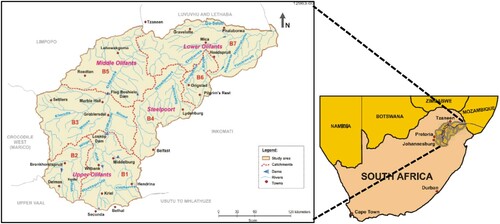
The Olifants Water Management Area (OWMA) is located in the north-eastern part of SA and falls within three provinces – Limpopo, Mpumalanga, and Gauteng provinces. It covers an area of about 54,570 km² with a total mean annual runoff of about 2,400 million m³ per annum. From the water management perspective, the catchment is divided into four sub-areas namely the Upper Olifants, Middle Olifants, Lower Olifants, and Steelpoort areas (see Figure 1). The varying economic activity in these areas has led to enormous water demand and deterioration of water quality making the catchment the third most water-stressed and most polluted in SA (DWS, 2011c; Wambui et al., 2016). For instance, extensive mining and coal-fired power generation supporting 48% of SA’s total power generation capacity are located in the Upper Olifants sub-area (UNEP, 2015). Accordingly, the Upper Olifants River is characterised by extensive pollution and acidification. Human settlements and agricultural activities (both commercial and subsistence, including the second-largest irrigation scheme in the country) are also located in the middle section of the catchment around the Loskop dam. Given the importance of the Olifants River to economic activities in the OWMA, there is a need to manage the water resource in a manner that ensures an equitable balance among the multiple users and uses. In this context, the OWMA was selected as a case study area (out of the nine water management areas in SA) to analyse the distributional implications of protecting the water resources in the catchment.

Figure 1. Location of the Olifants water management area and the four sub-areas. Source: DWS (2011b) and De Lange et al. (2005).

2.2. Specification of the regional CGE model

To analyse the distributional impacts of taxing water pollution in the OWMA, we adapted the International Food Policy Research Institute (IFPRI) standard static CGE model specifications of Löfgren et al. (2002)³ to the requirements of a regional model and integrated an environmental component. This subsection provides the general features of our regional environmental CGE model.⁴

Like all CGE models, our regional model is grounded in neoclassical theory on producer and consumer behaviour and describes the entire Olifants economy. Producers and consumers are assumed to behave rationally and their decisions determine the demand and supply of goods and services as well as factors of production. Producers maximise profits, defined as the difference between revenue and the cost of intermediate inputs, primary factors, pollution, and abatement. That is, the cost of production in our model includes pollution-related costs due to prescribed environmental standards. Profits are maximised subject to production technology, the choice of which follows a sequential process. At the first level of the technology nest, a Leontief function combines aggregate value-added and aggregate intermediate input to determine activity levels. At the second level of the nest, aggregate intermediate input is a Leontief function of the various individual intermediate inputs each of which is a constant elasticity of substitution (CES) function of a domestic commodity and its imported equivalent. Imported commodities include imports from the rest of the world (ROW)⁵ whereas exported domestic outputs are distinguished from those produced and sold in the study region using a constant elasticity of transformation (CET) function. Also, at the second level, a CES function combines different labour skills (unskilled, skilled, and highly skilled) and capital into aggregate value-added.

We assume that higher-skilled labour (highly skilled and skilled) and capital are fully employed with flexible real wages and capital rental prices. On the contrary, and to reflect the reality in the SA labour market, unskilled labour is assumed to be not in full employment at a fixed real wage. Each sector including the incorporated pollution abatement sectors produces one unique commodity and shares the same production structure except for the differences in input proportions and behavioural parameters.

All factor incomes are distributed to domestic institutions (households, government, and enterprise) in fixed factor-shares after transfer payments to the ROW, in foreign currency. In addition to factor incomes, households receive transfers from other institutions and spend their income on paying taxes, buying commodities, saving, and making transfers to other institutions. Household consumption demand is modelled as a linear expenditure system (LES) that differentiates between necessities and luxury commodities with the assumption that domestic and imported commodities are imperfect substitutes (Armington, 1969). The government collects revenue from taxes (including water pollution taxes) and transfers from the ROW. The government uses its income to finance public consumption and transfers to other institutions. Government consumption is assumed to be fixed in real terms, whereas its saving is determined residually. Trade with other regions in SA and foreign countries is allowed through transacting with the ROW sector. We adopt the standard assumption of a small open economy, thus, import and export prices are determined in the world market which is assumed to be big enough to absorb all exports and meet all import demands.

The environment in this study is captured through water pollution and abatement. Our model specification extends standard CGE formulations to include a production function for pollution abatement activities and treats their ‘output’ as special intermediate goods bought by polluters.⁶ The incorporated pollution abatement sectors have the responsibility of providing the best available cleaning or purification services to help polluters meet prescribed environmental standards. The amount paid by polluters for these special intermediate goods constitutes their abatement cost. Our model also assumes that not all pollution generated in the economy can be removed by the abatement sectors, so the government levies a tax on the amount not removed (unabated pollution). Therefore, the cost of pollution control which includes water pollution tax and abatement cost is included in the cost of production (i.e. based on the ‘polluter pays’ principle).

We consider three water pollutants (salinity, nitrogen, and phosphorus), and assume that pollution is generated proportional to output levels of each sector. Polluters also incur two types of pollution-related costs: water pollution tax and pollution abatement cost to comply with set water quality standards. The demand and price of pollution abatement services are endogenously determined in the model based on prevailing market conditions. The two main equations for adding pollution and pollution abatement activities to the model are as follows: (1) $PETA{X}_a=\sum _{g}tp{e}_g.d_{ga}.Q{A}_a.\left(1-c{l}_g\right)$(1) (2) $PACOS{T}_a=\sum _{g}PA{G}_g.d_{ga}.Q{A}_a.c{l}_g$(2) where $PETA{X}_a$ and $PACOS{T}_a$ are, respectively, the total cost of pollution taxes and pollution abatement services to sector a for discharging pollutant g. $d_{g,a}$is the production pollution coefficient of pollutant g in sector a, $Q{A}_a$ is the total output of sector a, $PA{G}_g$price of pollution clean-up services for pollutant g, $tp{e}_g$ is the per-unit tax levied by the government on discharging pollutant g, and $c{l}_g$ is the economy-wide cleanup rate of pollutant g (i.e. the proportion of pollutant g abated by producers’ in the economy as a result of purchasing abatement ‘commodities’). It is important to note that equations (1)(1) $PETA{X}_a=\sum _{g}tp{e}_g.d_{ga}.Q{A}_a.\left(1-c{l}_g\right)$(1) and (2)(2) $PACOS{T}_a=\sum _{g}PA{G}_g.d_{ga}.Q{A}_a.c{l}_g$(2) implicitly determine the quantities of pollution emitted and abated, respectively. The model also includes different pollution-related indicators such as the total amount of pollution abated/cleaned up and the amount of pollution discharged into the environment.

Finally, the model has a set of macro constraints (government balance, savings and investment balance, and the current account of the rest of the world) that must be satisfied by the system as a whole. Each macro constraint is governed by a set of closure rules that ensures that there is a balance between the number of endogenous variables and independent equations in the system (Löfgren, 1995). Given that it is difficult to argue for a single rule, we examine in our policy simulations’ section alternative macro closure scenarios to assess the distributional impacts of taxing water pollution in the OWMA.

2.3. Data and calibration

Our CGE model is calibrated to a regional dataset employing the social accounting matrix (SAM) structure (Round, 2003). A typical SAM, however, does not provide information on the interactions between economic activities and the environment. As pointed out by Bartelmus et al. (1991), a conventional SAM fails to represent the degradation of environmental quality caused mainly by pollution and the decumulation of natural resources that could threaten the sustained production of the economy. Thus, to assess the distributional impacts of taxing water pollution, a new integrated SAM which captures the relationships between economic and water pollution-related information was constructed for the basin using the framework of environmentally extended SAM developed by Xie⁷ (2000). The pollution-related information includes sectoral payments for pollution abatement services, pollution taxes, and pollution abatement subsidies. The integrated SAM serves as a consistent database for calibrating our environmental CGE model.

The SAM used for analysis is a consolidated version of three provincial SAMs for the year 2012. The initial SAMs were developed by the Development Bank of Southern Africa (DBSA) for the year 2006 (DWS, 2011b) and were updated for the year 2012 using information from statsSA. The consolidated SAM has ten producing sectors (aggregated from the 46 sectors’ provincial SAMs) with information on intermediate inputs, value-added, consumption, taxes, and trade. The aggregation of sectors was done based on the type of pollutant discharged into the environment. Sectors of our model include agriculture (disaggregated into field crops, horticulture crops, livestock, and other agriculture), mining, manufacturing (disaggregated into chemical manufacturing, wood and paper, food, beverage, and tobacco, and other manufacturing), and services. In addition to the ten producing sectors, the SAM is extended to include three pollutants (salinity, nitrogen, and phosphorus)⁸, and three corresponding pollution abatement sectors. Specifically, the conventional commodity by pollution abatement activity matrix contains intermediate inputs of pollution abatement sectors. On the other hand, the pollution abatement commodity by production activity matrix reflects sectoral demand for/or spending on pollution abatement services. Thus, pollution abatement services are treated as special intermediate goods and added to the commodity accounts. The entry in the activity by pollution abatement commodity shows the total value of pollution abatement service or pollution clean-up. Furthermore, our regional environmental SAM has three pollution tax accounts that receive payments from production sectors for their water pollution discharges. These taxes are transferred to the consolidated government account.

Because a SAM with water pollution information for the OWMA has not been built before, we adopt an indirect approach to estimate the pollution-related data by pollutant and sector. Using data from the DWS Water Management System (WMS) for the year 2012, we estimated the load for each pollutant at selected monitoring sites along the Olifants River using the volume of flow and median concentration for the month. The estimated load from the monitoring sites was summed to obtain the total load per pollutant for the base year. This was disaggregated by sector using the best available information (which includes information on spatial trends in pollutants and land use activities in the catchment) from previous studies (DWS, 2011b, 2011c; Dabrowski & de Klerk, 2013). The pollution intensities of each pollutant by sector were then calculated using data on sectoral output and pollution load. The cost of operating a standard treatment plant to reduce pollutants to achieve in-stream water quality was obtained from previous DWS studies in the OWMA (DWS, 2003, 2011b). These data were disaggregated using the estimated pollution intensities to obtain the pollution abatement cost of each production sector and for each pollutant.

Given the varying data sources, the initial environmental SAM was unbalanced, that is, it did not fulfil the row-column constraint. As a result, we employed the cross-entropy method (Robinson et al., 2001) to balance it using the General Algebraic Modelling System (GAMS) software (Brooke et al., 1998). The environmental model was then calibrated to the environmental SAM by first defining all prices to be equal to one as commonly done in the calibration approach. This implies that all price indices are indexed to the model’s base year and that sectoral flows in the environmental SAM measure both real and nominal magnitudes (Robinson et al., 1999). Factor returns were estimated based on the procedure described by Robinson et al. (1999) with factor quantities sourced from Hassan and Thurlow (2011). The model has two different types of parameters. The first which consists of share parameters like consumption shares and average tax and savings rates were determined from the data contained in the environmental SAM. The other set of parameter values comprises output and trade elasticities and were adopted from Hassan and Thurlow (2011). A sensitivity analysis employing different elasticity parameters was also conducted to check the robustness of the model.

To investigate distributional impacts, households were disaggregated into four income groups representative of those living in the study region, using monthly poverty lines (lower and upper-bounds) in 2018 prices from Statistics South Africa (StatsSA, 2018). Households with income levels below the lower-bound poverty line (R 785 per month) were grouped into the poorest category. A vulnerable household category has been defined to include those with incomes above the lower-bound poverty line but far below the upper-bound poverty line (i.e. between R 785 – R 825 per month). Note that these two groups (poorest and vulnerable) constitute more than 75% of the population in the OWMA (Table 1). Middle-income households were those with incomes far above the lower-bound poverty line (i.e. above R 825 – R 1183 per month) whereas High-income households were those above the upper-bound poverty line (R 1183 per month).

Table 1. Household income source and their tax shares (base year 2012).

Household	Household income (upper)	Labour income share				Capital income share	Transfer income share	Tax share of income	Population share
		Highly skilled	Skilled	Unskilled	Total labour income share
Poorest	10,600	0.00	0.11	0.55	0.66	0.17	0.18	0.085	0.26
Vulnerable	18,400	0.19	0.13	0.17	0.50	0.44	0.06	0.103	0.51
Middle income	38,000	0.24	0.17	0.08	0.49	0.47	0.05	0.105	0.12
High income	Above 38,000	0.28	0.10	0.00	0.38	0.61	0.01	0.126	0.09

Source: Olifants environmental SAM (Kyei, 2019) and DWS, 2011b; Notes: Household income is in Rands per annum. Also, the sum of the shares may be smaller/greater than 1 due to rounding.

3. Results and discussion

We begin this section with a brief description of the household groups in terms of sources of income and expenditure. We then describe our policy scenarios in section 3.1 and follow that with the respective results and discussion.

As Table 1 shows, sources of income in the study area vary significantly between the above-defined income groups. High-income households derive a significant share of their income from highly skilled labour and capital, whereas the poorest households derive the bulk of their income from unskilled labour and transfers (both government and inter-institutional). On the consumption expenditure side, Table 2 indicates that the share of pollution-intensive goods in the consumption basket of poorest households is greater than that of high-income households. As will become clear in the subsequent policy simulation analysis, these structural features (household sources of income and share of pollution-intensive goods in household consumption basket) are key determinants of the distributional impacts (burden) of taxing water pollution in the river basin.

Table 2. Household consumption shares (base year 2012).

Household	Field crops	Horticultural crops	Livestock	Other agriculture	Chemical manufacturing	Food, beverage, and tobacco	Wood and paper	Other manufacturing	Services	Share of pollution-intensive goods in the household consumption basket^1
Poorest	0.11	0.03	0.02	0.07	0.08	0.32	0.05	0.14	0.18	0.64
Vulnerable	0.04	0.02	0.01	0.04	0.10	0.28	0.08	0.14	0.31	0.61
Middle income	0.03	0.01	0.02	0.03	0.06	0.23	0.06	0.22	0.36	0.59
High income	0.01	0.03	0.05	0.01	0.01	0.20	0.05	0.16	0.49	0.50

Source: Olifants environmental SAM (Kyei, 2019); Notes: Mining as a final consumption good is omitted from households’ consumption basket because in our SAM mining was used to only meet intermediate, export, and investment demands. Also, the sum of the shares may be smaller/greater than 1 due to rounding.

¹Pollution-intensive goods in our model include horticultural crops, livestock, mining, chemical manufacturing, food, beverage, and tobacco, wood and paper, and other manufacturing. Thus, the shares in the final column were obtained by summing the household consumption shares relating to pollution-intensive goods.

3.1. Distributional impacts of the water pollution tax and results of the remedial policy simulations’ scenarios

We used the environmental CGE model developed for the OWMA to assess the distributional impact of a water pollution tax to reduce nutrient load (total nitrogen and total phosphorus) in the study region. We assumed arbitrarily that the government raises the pollution tax rate on nutrient load by 50% with reference to the base value. We ran three policy scenarios. The first scenario assumed that all revenue generated from the pollution tax is absorbed in the government budget balance. This was intended to reveal the absolute incidence⁹ of the tax or the direction of the distributional cost when the tax revenue is used for fiscal adjustments such as reducing the budget deficit. The results of this experiment are reported under the ‘no-revenue recycling’ scenario. Implications of two other policy scenarios for the differential incidence of the pollution tax have been analysed to compare alternative remedial options for recycling the tax revenue. One of the complementary policies tested was to reinject the pollution tax proceeds back into the economic system by recycling all revenue through a direct subsidy to consumers as a lump-sum transfer to households. The second tax revenue recycling regime was to return the tax revenue to pollution abatement sectors in the form of a production subsidy.

3.2. Aggregate impacts of the water pollution tax

Table 3 shows the aggregate impact of the pollution tax on total nitrogen discharged, aggregate welfare¹⁰, as well as factor returns in the three policy scenarios. The result indicates that the pollution tax achieves its purpose of reducing nitrogen emissions by shifting production away from pollution-intensive sectors. Aggregate welfare which is measured by the Hicksian equivalent variation decreased under the no-revenue recycling scenario compared with the revenue recycling scenarios. Of the two revenue recycling scenarios, uniform government transfers to households outperform production subsidy to pollution abatement sectors. The reason is that the uniform government transfer which is a direct subsidy to households’ boosts their income and enhances the demand for consumption goods via higher purchasing power. On the other hand, the subsidy to pollution abatement sectors reduces the cost of their production, thus boosting the capacity of the regional economy to clean up. It should, however, be noted that losses in household welfare only reflect changes in consumption because the benefits of water quality improvements are not considered in their utility function. Our welfare results can, therefore, be considered as a lower bound on the welfare gains from improving water quality in the Olifants river basin.

Table 3. Aggregate impact of a 50% increase in pollution tax on Nitrogen emission under alternative revenue recycling scenarios (in %age change).

	No-revenue recycling	Uniform transfers to households	Production subsidy to pollution abatement sectors
Total nitrogen discharged	−0.330	−0.260	−0.210
Welfare	−0.058	0.044	−0.006
Wage rate highly skilled labour	−0.210	−0.153	−0.070
Wage rate skilled labour	−0.263	−0.188	−0.081
Capital rental price	−0.319	−0.216	−0.098

Source: Olifants environmental CGE model, (Kyei, 2019).

3.3. Distributional impacts and remedial policy options

3.3.1. Without revenue recycling

The distributional impact of the water pollution tax on households differs as a result of differences in spending and income patterns. The pollution tax affects the relative prices of pollution-intensive and non-polluting goods (spending side) as well as the returns to capital and labour (income side). The impact on factor returns depends on the factor intensity of each sector thus; the relative contribution of the different factor endowments on household income drives the distributional results from the income side.

The immediate impact of introducing the pollution tax is an increase in the marginal cost of production in polluting sectors, causing them to re-optimize to lower output levels. This negatively impacts demand for primary factors, particularly capital, since polluting firms are relatively capital intensive. Although, prices of both capital and labour fall, capital bears the bigger burden of the tax increases (see Table 3), because the reduction in capital by polluting firms outweighs the reduction in labour. All households experience a fall in income due to lower remuneration to factors of production. However, wealthy households experience a larger fall in income because of a bigger fall in the relative return to capital and the fact that they derive a greater share of their income from capital endowments (see Table 1). Poor households, on the other hand, receive a greater share of their income from labour, mainly unskilled labour and transfers which is fixed because it is indexed to inflation. Although the impact of the tax on the vulnerable group is also high, the share of total income for both the poorest and vulnerable groups increases after the tax (see column 3 of Table 4). Therefore, the distributional impact of the pollution tax is progressive from the income side (i.e. poor households are less affected by the changes in factor prices).

Table 4. Impact of the water pollution tax on income, consumer spending, and net income (without revenue recycling).

Households	Share in total income before tax	Share in total income after tax	%age change in income after tax	Equivalent variation	Net income
Poorest	0.141	0.151	−0.167	−0.021	−2.662
Vulnerable	0.150	0.154	−0.204	−0.015	−1.665
Middle income	0.159	0.158	−0.227	−0.012	−1.662
High income	0.551	0.537	−0.243	−0.010	−1.138

Source: Olifants environmental CGE model, (Kyei, 2019).

From the consumption point of view, the imposition of the pollution tax raises the price of pollution-intensive goods causing households to reduce the share of pollution-intensive goods in their consumption basket (i.e. demand for pollution-intensive goods fall by a greater percentage compared with non-polluting goods). However, the increase in the prices of pollution-intensive goods adversely affects the poor than the rich, because the former allocate a greater share of their expenditure on pollution-intensive goods (see Table 2). As mentioned earlier, the Hicksian equivalent variation¹¹ was used as a welfare indicator to assess the distributional impact from the spending side. Column 5 of Table 4 shows that poor households would be willing to pay twice as much as rich households to avoid the implementation of the water pollution tax policy. This suggests that from the spending side, the pollution tax is not pro-poor because it hurts the poor more than the rich (i.e. it’s regressive).

Given that the pollution tax is poverty-reducing from the income side and poverty increasing from the expenditure side, we assess its net impact using net income (i.e. the difference between income and expenditure). The last column of Table 4 indicates that the negative impact on the expenditure side more than offset the positive impact on the income side. As a result, the introduction of a water pollution tax in the Olifants river basin without revenue recycling will hurt the poor. Our result is consistent with the literature on the distributional impact of carbon/energy taxes which argues that the distributional impact of these taxes is due to the higher pollution-intensive or energy expenditure share of poor households.

3.3.2. Under revenue recycling

In this subsection, we discuss the results of two revenue recycling options employed to offset the negative impact of the tax policy on the poor. Overall, recycling the pollution tax revenue improves the welfare of all households with the poor gaining more from the redistribution. For instance, under the government transfers to households recycling option, poor households would be willing to pay at most R 78,000 to see the implementation of the pollution tax policy whereas rich households would be willing to pay a maximum amount of R 105,000 to avoid the lower utility level due to the pollution tax policy (see column 5 of Table 5).¹² Also, column 2 of Table 5 indicates that poor households increase their share in total income after the introduction of the pollution tax relative to rich households. Thus, recycling the tax revenue will have a positive impact on equity by redistributing income from the better-off to the poor and vulnerable. The lower impact of the production subsidy recycling option is caused by the restrictive specification of the fixed coefficients Leontief production technology, which does not allow substitution flexibility between inputs. Production activities in our model buy abatement for only a fixed ratio of total pollution generated and the remainder is disposed of in the environment, making the supply of pollutants move in direct proportion to the level of economic activity.

Table 5. Impact of the pollution tax on income, consumer spending, and net income (with revenue recycling).

Uniform transfers to households
Households	Share in total income before tax	Share in total income after tax	%age change in income after tax	Equivalent variation	Net income
Poorest	0.141	0.195	0.423	0.078	0.150
Vulnerable	0.150	0.179	0.219	0.038	0.094
Middle income	0.159	0.184	0.183	0.035	0.094
High income	0.551	0.443	−0.177	−0.105	0.064
Production subsidy to pollution abatement sectors
Poorest	0.141	0.146	−0.026	−0.005	−0.357
Vulnerable	0.150	0.153	−0.043	−0.004	−0.521
Middle income	0.159	0.159	−0.063	−0.007	−0.522
High income	0.551	0.542	−0.077	−0.011	−0.835

Source: Olifants environmental CGE model, (Kyei, 2019).

Our findings, in a nutshell, suggest that taxing water pollution in the Olifants river basin without complementary measures to address the potential negative impact would lead to socially undesirable outcomes. However, recycling the tax revenue would mitigate the adverse social impact of the water pollution tax with a trade-off between improving the current welfare of the basin’s population and boosting the capacity of the regional economy to clean up its pollution.

4. Conclusions and implications for research and policy

Using the Olifants river basin as a case study, this paper developed and used a regional environmental CGE model to assess the distributional impact of a water pollution tax considering both the income and spending-side effects. We also analysed the distributional impact of two revenue recycling schemes to mitigate the potential adverse effect of the policy. Our CGE model was calibrated using an extended SAM database that integrates water pollution abatement activities for the Olifants basin.

Results of our analysis indicate that without revenue recycling, the water pollution tax is progressive (inequity and poverty-reducing) from the household income perspective but regressive (inequity and poverty increasing) from the household spending perspective. The net impact is, however, regressive showing that the spending-side effect dominates the income-side effect. This finding stems from the large expenditure share of pollution-intensive goods in the consumption basket of poor households compared to the rich in the basin. Depending on the revenue recycling scheme, the regressive effect of the pollution tax is either weaken or reversed. Recycling the tax revenue through government transfers to households leads to progressive welfare outcomes, whereas returning the tax revenue to pollution abatement sectors in the form of a production subsidy weakens the regressive effect. The weak impact of the production subsidy recycling option is due to rigidities on the production side of our model. Nonetheless, our finding is consistent with the literature and highlights the need to analyse the distributional impacts of environmental policies from both the income and spending sides. Also, the results suggest a high potential for fiscal policy regimes to mitigate the socioeconomic burden of the water pollution tax on households’ welfare.

However, the findings should be interpreted with caution because by modelling the demand for pollution abatement services with a Leontief production function, we assumed that the unit costs of pollution abatement are fixed. This rigid assumption should be relaxed in future research as better data becomes available. Moreover, our analysis does not consider the economic benefits from water quality improvements or water pollution reduction technologies.

Disclosure statement

No potential conflict of interest was reported by the author(s).

Notes

1 In CGE modelling, two methods exist for analysing the impacts of policy interventions on the distribution of incomes across households. The first is the traditional method where the household sector is disaggregated into a number of representative households normally based on considerations like income and characteristics of the household head. The second is the micro-simulation method where the CGE model is integrated with a household module in which the units correspond to individual household observations in a nationally representative survey (Löfgren et al., 2003). The household module may be fully integrated with the CGE model or sequentially linked to it. Due to lack of data and for our purposes, we employ the representative household method.

2 Equivalent variation measures the change in expenditure at base year prices that would be equivalent to the policy implied change in utility. Put differently, it measures the monetary value of a change in utility for a given household as a result of introducing the water pollution tax.

3 Due to lack of data, we omit certain features of the generic model. For example, our model does not include home consumption of domestically produced goods and the assumption that activities produce multiple products. It is important to note that the omission of these features does not impact on the validity of our model. Also, the regionalisation of the model involved the construction of a regional SAM and adopting new closure rules for the accounts of the government and the rest of the world.

4 See, Kyei (2019) for a detailed description of the Olifants environmental CGE model.

5 ROW in this case includes all other regions in SA (i.e., outside study region), in addition to foreign countries.

6 The environmental component of our model follows closely that of Xie & Saltzman (2000). We, however, exclude certain features such as consumption pollution because of data limitations, and since production activities constitute the major source of pollution in our case study area – the OWMA (DWS, 2011c).

7 Xie (2000) developed a framework for extending a SAM to include pollution-related information such as pollution abatement activities, sectoral payments for pollution abatement services, pollution emission taxes, pollution abatement subsidies and environmental investment.

8 These constitute the major pollutants in our case study region (DWS, 2011c; Dabrowski & de Klerk, 2013).

9 Fullerton and Metcalf (2002) distinguished three tax incidences in terms of distributional effects: absolute, balanced budget and differential.

10 Aggregate welfare is a simple sum of the welfare results for all household groups. That is, we did not apply a weighting scheme. Also, we report here only the simulation results for nitrogen due to space limitations and the fact that results for the other pollutants follow a similar trend.

11 The formula used was adapted from Blonigen et al. (1997).

12 Values in column 5 were multiplied by 1000 to obtain the willingness to pay amounts since our base year units were in millions of Rands (except for employment and pollutants discharged).

References

- Alton, T, Arndt, C, Davies, R, Hartley, F, Makrelov, K, Thurlow, J & Ubogu, D, 2014. Introducing carbon taxes in South Africa. Applied Energy 116, 344–54.
- Armington, PS, 1969. A theory of demand for products distinguished by place of production. IMF Staff Papers 16, 159–78.
- Baranzini, A, Goldemberg, J & Speck, S, 2000. A future for carbon taxes. Ecological Economics 32(3), 395–412.
- Bartelmus, P, Stahmer, C & Tongeren, JV, 1991. Integrated environmental and economic accounting: framework for a SNA satellite system. Review of Income and Wealth 37(2), 111–48.
- Beck, M, Rivers, N, Wigle, R & Yonezawa, H, 2015. Carbon tax and revenue recycling: impacts on households in British Columbia. Resource and Energy Economics 41, 40–69.
- Blonigen, B, Flynn, JE, & Reinert, KA, 1997. Sector-focused general equilibrium modeling. In J, Francois & K, Reinert (Eds.), Applied methods for trade policy analysis: A handbook, Cambridge, Cambridge University Press, 189–230. https://doi.org/https://doi.org/10.1017/CBO9781139174824.009
- Bovenberg, AL & Goulder, LH, 2002. Environmental taxation and regulation. In Handbook of public economics, Vol. 3, Elsevier, 1471–1545.
- Brannlund, R & Nordstrom, J, 2004. Carbon Tax simulations using a household demand model. European Economic Review 48(1), 211–33.
- Brooke, A, Kendrick, D, Meeraus, A, Raman, R & America, U, 1998. The general algebraic modeling system. GAMS Development Corporation, 1050.
- Brouwer, R, Hofkes, M & Linderhof, V, 2008. General equilibrium modelling of the direct and indirect economic impacts of water quality improvements in the Netherlands at national and river basin scale. Ecological Economics 66(1), 127–40.
- Dabrowski, JM & de Klerk, LP, 2013. An assessment of the impact of different land use activities on water quality in the upper Olifants river catchment. Water SA 39(2), 231–44.
- De Lange, M, Merrey, DJ, Levite, H & Svendsen, M, 2005. 9 Water Resources Planning and Management in the Olifants Basin of South. Irrigation and river basin management: Options for governance and institutions, 145.
- Devarajan, S, Go, DS, Robinson, S & Thierfelder, K, 2011. Tax policy to reduce carbon emissions in a distorted economy: illustrations from a South Africa CGE model. The BE Journal of Economic Analysis & Policy 11(1): Article 13. https://doi.org/https://doi.org/10.2202/1935-1682.2376.
- Dinan, TM & Rogers, DL, 2002. Distributional effects of carbon allowance trading: how government decisions determine winners and losers. National Tax Journal, 55(2), 199–221.
- DWS (Department of Water and Sanitation), 2003. Water Quality Management Series. Sub-Series No. MS11. Towards a Strategy for a Waste Discharge Charge System. First Edition. Pretoria.
- DWS (Department of Water and Sanitation), 2011a. Directorate Water Resource Planning Systems: Water Quality Planning. Resource Directed Management of Water Quality. Planning Level Review of Water Quality in South Africa. Sub-series No.WQP 2.0. Pretoria, South Africa.
- DWS (Department of Water and Sanitation), 2011b. Classification of Significant Water Resources in the Olifants Water Management Area (WMA 4): Report 3a: Report on IUAs and Report on Socio-economic evaluation framework and the decision-analysis framework. Report 3b: Analysis scoring system. RDM/WMA04/00/CON/CLA/0311.
- DWS (Department of Water and Sanitation), 2011c. Water Quality Report: Development of a reconciliation strategy for the Olifants river water supply system. Report number: P WMA 04/B50/00/8310/7.
- Fullerton, D & Metcalf, GE, 2002. Tax incidence. Handbook of Public Economics 4, 1787–872.
- Goulder, LH, 1998. Environmental Policy making In A second-best setting. Journal of Applied Economics 1(2), 279–328.
- Hamilton, K & Cameron, G, 1994. Simulating the distributional effects of a Canadian carbon Tax. Canadian Public Policy 20(4), 385–99.
- Hassan, R & Thurlow, J, 2011. Macro-micro feedback links of water management in South Africa: CGE analyses of selected policy regimes. Agricultural Economics 42(2), 235–47.
- Kerkhof, AC, Moll, HC, Drissen, E & Wilting, HC, 2008. Taxation of multiple greenhouse gases and the effects on income distribution: a case study of the Netherlands. Ecological Economics 67(2), 318–26.
- Kyei, C & Hassan, R, 2019. Managing the trade-off between economic growth and protection of environmental quality: the case of taxing water pollution in the Olifants river basin of South Africa. Water Policy 21(2), 277–90.
- Kyei, CK, 2019. Economy-wide implications of water quality management policies: a case of the Olifants river basin, South Africa. Ph.D Thesis, University of Pretoria, Pretoria, South Africa.
- Löfgren, H, 1995. Macro and micro effects of subsidy cuts: A short-run CGE analysis for Egypt. TMD discussion paper no. 5.
- Löfgren, H, Harris, RL, Robinson, S, El-Said, M & Thomas, M, 2002. A standard Computable general equilibrium (CGE) model in GAMS. microcomputers in Policy Research, Vol. 5. IFPRI, Washington, D.C.
- Löfgren, H, Harris, RL, Robinson, S, & El-Said, M, 2003. Poverty and inequality analysis in a general equilibrium framework: the representative household approach. In F, Bourguignon & LA, Pereira da Silva (Eds.), The impact of economic policies on poverty and income distribution: Evaluation techniques and tools, World Bank, Oxford University Press, 325-337.
- National Treasury, 2013. Carbon Tax Policy May 2013. [Online]. http://www.treasury.gov.za/public%20comments/Carbon%20Tax%20Policy%20Paper%202013.pdf (Accessed 5 December 2019).
- O'Ryan, R, de Miguel, CJ, Miller, S & Munasinghe, M, 2005. Computable general equilibrium model analysis of economywide cross effects of social and environmental policies in Chile. Ecological Economics 54(4), 447–72.
- Ojha, VP, 2009. Carbon emissions reduction strategies and poverty alleviation in India. Environment and Development Economics 14(3), 323–348.
- Oladosu, G & Rose, A, 2007. Income distribution impacts of climate change mitigation policy in the susquehanna river basin economy. Energy Economics 29(3), 520–44.
- Pearson, M & Smith, S, 1991. The European carbon Tax: An assessment of the European commission’s proposals. The Institute for Fiscal Studies, London.
- Poterba, JM, 1991. Is the Gasoline Tax Regressive?. NBER Working Papers No 3578.
- Rausch, S, Metcalf, GE & Reilly, JM, 2011. Distributional impacts of carbon pricing: A general equilibrium approach with micro-data for households. Energy Economics 33, S20–S33.
- Rausch, S, Metcalf, GE, Reilly, JM & Paltsev, S, 2010. Distributional implications of alternative US greenhouse gas control measures. The BE Journal of Economic Analysis & Policy 10(2), Article 1. https://doi.org/https://doi.org/10.2202/1935-1682.2537.
- Robinson, S, Cattaneo, A & El-Said, M, 2001. Updating and estimating a social accounting matrix using cross entropy methods. Economic Systems Research 13(1), 47–64.
- Robinson, S, Yùnez-Naude, A, Hinojosa-Ojeda, R, Lewis, JD & Devarajan, S, 1999. From stylized to applied models: building multisector CGE models for policy analysis. The North American Journal of Economics and Finance 10(1), 5–38.
- Round, J, 2003. Social accounting matrices and SAM-based multiplier analysis. The impact of economic policies on poverty and income distribution: Evaluation techniques and tools. World Bank and Oxford University Press, New York, 261–76.
- StatsSA (Statistics South Africa), 2018. National poverty lines. Statistical release P0310.1.
- UNEP (United Nations Environment Programme), 2015. Global Synthesis Report of the Project for Ecosystem Services, Ecosystem Services Economics Unit, Division of Environmental Policy Implementation. https://reliefweb.int/sites/reliefweb.int/files/resources/Global%20synthesis%20report.pdf (Accessed 5 December 2019).
- Van Heerden, J, Blignaut, J, Bohlmann, H, Cartwright, A, Diederichs, N & Mander, M, 2016. The economic and environmental effects of a carbon tax in South Africa: A dynamic CGE modelling approach. South African Journal of Economic and Management Sciences 19(5), 714–32.
- Van Heerden, J, Gerlagh, R, Blignaut, J, Horridge, M, Hess, S, Mabugu, R & Mabugu, M, 2006. Searching for triple dividends in South Africa: fighting CO₂ pollution and poverty while promoting growth. The Energy Journal, 27(2), 113–41.
- Wambui, G, Thiam, DR & Kanyoka, P, 2016. Economic analysis of water policy reforms in South Africa: The case of the Olifants river basin. Center for Development Research (ZEF), University of Bonn, Germany.
- Wang, Q, Hubacek, K, Feng, K, Wei, YM & Liang, QM, 2016. Distributional effects of carbon taxation. Applied Energy 184, 1123–31.
- Wier, M, Birr-Pedersen, K, Jacobsen, HK & Klok, J, 2005. Are CO2 taxes regressive? evidence from the danish experience. Ecological Economics 52(2), 239–51.
- Xie, J, 2000. An environmentally extended social accounting matrix. Environmental and Resource Economics 16(4), 391–406.
- Xie, J, & Saltzman, S, 2000. Environmental policy analysis: An environmental computable general-equilibrium approach for developing countries. Journal of Policy Modelling, 22(4), 453–489.
- Yusuf, AA & Resosudarmo, BP, 2015. On the distributional impact of a carbon tax in developing countries: the case of Indonesia. Environmental Economics and Policy Studies 17(1), 131–56.