IDENTIFYING THE DRIVERS OF TRADE FINANCE IN SOUTH AFRICA

Abstract

Trade finance (or bank intermediated trade finance) plays an integral role in facilitating trade across the globe: most studies assert that trade finance (TF) forms part of more than 80% of total global trade. Although TF has increased in importance for policy makers after the financial crises of 2008, most studies conducted over the last decade (2009 onward) focussed on the supply side of TF and how its reduction has hampered trade. By applying a robust least squares maximum likelihood estimation technique, and using bi-squares and median absolute deviation-centred (MADMED) scaling, this study investigates the international and domestic variables driving demand for TF for several listed South African companies. This study identified 12 instances of individually significant relationships between certain industries and the independent variable (both domestic and international financial and economic variables). It also found significant regression results for the retail industry at first differences and identified that macro-economic and financial variables (such as the US gross domestic product and the rand-British pound exchange rate) influenced the demand for retail TF. The sole significant domestic variable was South African bank asset-to-capital ratios, showing that both financial and economic factors are relevant in identifying TF demand drivers of South African companies.

1 Introduction

In 2017 a study conducted by the World Trade Organisation (WTO) found that its members had participated in commercial merchandise exports to the value of US$17,3tn (WTO, 2018). Currently (2019), very little is understood regarding the components and drivers of trade finance (TF) flows between countries and regions: there is no comprehensive study which connects TF demand to robust explanatory variables (Auboin, 2016:4). This creates the opportunity for a deeper investigation into the drivers of TF and the nature of these variables.

The goal of this study – namely to establish a robust regression model which identifies and assesses the significance of principal explanatory constituents of South African TF demand – becomes even more pressing when we consider that approximately 80% of global trade relies on some version of TF (Liston & McNeil, 2013:2). By applying a more country-specific, firm-oriented approach, this study aims to contribute to the small pool of knowledge that has to date only identified historical banking crises as influencers and drivers of TF volumes (Ronci, 2004:16). Identifying additional components of TF is of paramount importance to both policy makers (hoping to bolster trade in their respective countries), and financial service providers (who will be able to forecast the needs of their clients with greater accuracy). The remainder of this study proceeds as follows: Section 2 presents the literature governing TF and problems currently facing TF. Section 3 is the data section, while Section 4 covers the methodology and describes the model used to regress these data. Section 5 presents and discusses the results and Section 6 concludes.

2 Literature overview

TF is estimated to constitute between 80% and 90% of annual global trade (Liston & McNeil 2013:2), but Kathuria and Malouche (2016:222) point out that most of this trade occurs without bank intermediation. This may lead to the conclusion that there is no compelling need for banks in the international trade system, but this would be incorrect. Many companies do conduct trade on an open account basis, in which exporters ship goods to customers with payment taking place after an agreed-upon period. This is then accompanied by the use of TF instruments such as supply chain finance (SCF), which are facilitated by the banking/financial sector. The International Chamber of Commerce (ICC) has seen a growth in usage of SCF by companies in recent years (ICC, 2016). What is not mentioned is that this use of open account finance is only used in instances where trade relationships already exist as well as in more developed economies (Kathuria & Malouche, 2016:222), as the risks of non-payment are substantially increased with open account trading. Open account finance is very rarely used in connection with trade to lower income countries, where the perceived political and economic risks are considered high.

This highlights the importance of banks, which, through intermediation and various TF instruments, help smooth over the initial stages of exporting (Kutharia & Malouche, 2016:221), particularly in circumstances where companies have no previous established business relationships nor history to draw upon. This assistance therefore allows new exporters and importers to cultivate business relationships to the point where the contractual nature of their business dealings could improve (Defever, Fischer & Suedekum, 2016) and allow for a more versatile and flexible system of finance to develop. This is why it is important that policy makers understand what factors contribute to driving the demand for TF in the domestic market, and what policy initiatives can be taken to help facilitate access to TF for small and medium enterprises (SMEs), especially considering that SMEs have typically been excluded from TF markets through low application approval rates (Auboin, 2015:3ii). Current literature and statistics surrounding the composition, market size and determinants of TF in particular, are scarce in some respects and non-existent in others. This dearth of information inhibits the ability of policy makers to craft effective government initiatives aimed at increasing the access to TF for these SMEs (BIS, 2014).

Little empirical work has been undertaken to explore the possible relationship between TF and trade volumes (Kohler & Savile, 2011:4). Studies do, however, exist which focus on historical TF flows and their reactions to market shocks. More specifically, some research investigates the supply of TF and how that supply is affected during market crashes, such as the credit crisis which triggered the 2008 to 2010 recession. TF volumes have been found to experience a large reduction in supply when faced with financial market distress, where studies found a marked decrease in TF, especially trade-related TF such as bank-intermediated transactions (Ronci, 2004:3). This was confirmed during the 2008-10 financial crisis where emerging markets saw a large decline in the availability of access to TF (IMF, 2009). The decrease in TF stemming from the 2008-10 financial crisis has been estimated to account for 15% to 20% of the decline in trade during that period (BIS, 2014). This reduction in TF was the second largest cause of the collapse in trade volumes, which in their peak saw a fall in exports since that of the great depression (Contessi & Nicole, 2012:5). It is interesting to note, however, that TF (as a percentage of total trade) increased during this period, as TF decreased at a smaller percentage than trade values. Indeed, even facing various supply constraints, such as increased risk aversion by banks, TF volumes remained somewhat stable as businesses were happy to off-load their default-risk to banks, even in the face of increased transaction costs (Asmundson, Dorsey, Khachatryan, Niculcea & Saito, 2011:13). Studies have also found total trade value and TF volumes to be positively correlated (Liston & McNeil 2013:1) with a 1% increase in TF leading to a 0,4% increase in imports (Auboin & Engemann, 2014). It is this correlation between TF access and trade volumes that forms the basis for G20 countries' plans to increase their capacity for TF in member states in the wake of the global recession, in hopes of restarting a recovery of total trade volumes that had drastically declined during that period (Auboin, 2016:6). It should be noted however, that the decline in trade during the 2008-10 recession was not caused by a decline in TF volumes or access, but a substantial demand shock amongst consumers (Asmundson et al., 2011:29).

Because TF plays an integral part in driving trade, it is necessary to highlight some disparities between countries and companies themselves. A study which included 45 African countries and 247 African commercial banks, found that the market for bank-intermediated TF (in 2014) was estimated to be valued at between US$330bn to US$350bn (African Development Bank, 2014). The worrying aspect of the study, however, was the value of unmet demand for TF on the African continent, which in 2011 was US$110bn and had increased to US$120bn in 2012 (African Development Bank 2014). The Asian Development Bank has estimated that the global unmet TF demand for the preceding year could be as high as US$1,9tn (Auboin, 2015:3ii).

Closer examination of TF statistics on a company level shows that large multinational companies (and especially their subsidiaries) have large advantages in the financial markets when compared to their SME competitors. With the large multinationals with a larger approval rate for their TF applications, where only 7% of applications are rejected compared to the 50% of applications that are rejected for SMEs (Auboin 2015:3ii). This is puzzling, in that the average transaction default rate for short-term trade credit is only 0,1% of which more than half is recovered from the sale of the underlying assets (International Chamber of Commerce 2013). This low rate of “loss given default” (LGD) can also be attributed to the fact that TF is “highly collateralised”, meaning that credit and insurance is usually provided against the sale of specific products which value can be easily measured and liquidated (Chauffour & Farole, 2009:7). This could serve as the starting point for possible policy decisions made by lawmakers concerning the access, or lack of access, that SMEs have to, especially when considering that causality has been established between a firms’ ability to export and its access to TF (Amiti & Weinstein 2011:VII), and that there exists a causal link between trade and TF at a macro level (Auboin & Engemaqnn, 2014).

Another problem with TF is the influence of the current Basel regulations (Chauffour & Farole, 2009; Buckley et al¹., 2014; Kathuria & Malouche 2016). The Basel II accord introduced problematical credit risk measures, increasing the sensitivity for capital risk requirements in a risk fraught economic environment of the global crisis (Chauffour & Farole, 2009:8). This, in conjunction with the downgrades of companies during the crisis, further reduced the access to TF for SMEs and banks in “risky” emerging markets. Though the regulations and risk measures set out in Basel II are still in place, there have been many additions and improvements to these measures through Basel III, which have created its own set of problems.

“The international standards of financial regulations [Meaning Basel III] are based on the experiences of the financial crises in the US and Europe, and do not necessarily reflect the conditions of the financial sectors in Asian emerging countries” (Buckley et al., 2014:115).”

This negative sentiment before Basel III's final implementation makes sense in light of the fact that Asian markets are the destination for the majority of all issued global letters of credits (Buckley et al., 2014; ICC, 2016). The more stringent regulations and larger capital requirements set out in Basel III have driven up costs of TF in emerging Asian economies whose financial positions are already precarious (Buckley et al., 2014:115). This assertion is confirmed by a survey conducted by the Asian Development Bank, where 79% of banks stated that the Basel regulatory framework played a significant role in hampering TF. Banks also stated the need to reduce TF supply by 5% if Basel III was implemented (Asian Development Bank, 2014).

This leads to the study's focus, namely, drivers of TF demand for listed South African companies. The drivers of variations in TF demand are still somewhat vague and the lack of research in this field has hampered governments and regulatory bodies (such as the Bank for International Settlements) from establishing risk-reduction policies without negatively affecting firm’s access to TF. The lack of research has also been a factor hampering firms’ ability to trade which also negatively affects economic growth.

3 3.Data

3.1 Independent variables

The lack of literature on TF presents particular challenges to econometric modelling. There is not an established set of explanatory variables. This study draws from previously established variables tested in the working paper of Garralda, Vasishtha & Garima (2015-2018:9), that included both international (to account for the effect of global market conditions) and domestic (to identify regional specific determinants of TF) variables, but also included various novel variables such as:

• Rand to US dollar exchange rate;²

• Rand to British pound exchange rate;³

• the capital-to-asset ratio for South African banks;⁴

• the total exports for South Africa;⁵

• nominal GDP growth for South Africa;⁶

• South Africa’s sovereign credit rating⁷ that has been quantified using a scale created by assigning a numerical value to each letter on the rating scale, with the worst rating receiving the lowest and the highest letter rating receiving the highest numerical value.

• South African financial condition index⁸. A financial condition index (FCI), is a comprehensive index that is constructed through the combining of various economic- and financial variables and can improve on the shortages experienced by other indexes in predicting economic trends (Zheng & Yu, 2014:33). South Africa’s FCI is constructed using five variables: real interest rates; the yield curve; earnings yield on shares; excess money supply growth; and real effective exchange rate change. (Quantec, 2019)

• the capital-to-asset ratio for US banks;⁹

• US financial condition index,¹⁰ which was gathered from the Federal Reserve Bank of St Louis and monitors the condition of US money-, debt- and equity markets (Federal Reserve of St Louis, 2020)

• US GDP growth;¹¹ and

• the VIX index.¹² An index that calculates the constant 30 day expected market volatility of the US stock market, derived from S&P 500 Index call and put prices (Chicago Board Options Exchange, 2020).

*Data sources available in footnotes.

Of the variables included, only the exchange rates were not used by Garralda, Vasishtha & Garima (2015-2018). These variables were included to capture the possible effect that currency fluctuations may have on the demand for TF, with the US Dollar exchange rate being included as it is the most traded currency globally. The British Pound exchange rate was included in this study because of the interconnected nature of the Johannesburg Stock Exchange (JSE) and the London Stock Exchange (LSE), with many major corporations being dual listed on both exchanges.

3.2 Dependent variable

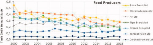
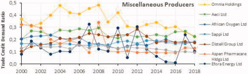
To obtain the dependent variable¹³, this study uses the approach of Dary and Haruna (2019). In particular, the dependent variable is taken as a company’s total trade payables for a given year, divided by its total assets for that same year, to obtain the individual company’s trade credit demand ratio (TCDR). These ratios were then grouped together according to their industry into different datasets, spanning 2000 – 2018, to allow a more accurate representation of individual business sectors. These companies were grouped according to the criteria listed below. They must be

• listed on the Johannesburg Stock Exchange (JSE);

• listed on the JSE involved in the retail sector;

• listed on the JSE involved in the mining sector;

• listed on the JSE falling within the classification of food producers;

• listed on the JSE classified as technology companies;

• producers, but do not fall within the larger groupings of producers.

In total, 41 South African companies, sorted into five distinct groupings, were used. These are visualised, along with their respective TCDRs, in Annexure 5. Annexure 5 also serves to showcase this study’s modelling considerations, in which outlier data points and high volatility of certain companies had to be considered when selecting the most appropriate model for regression.

3.3 A preliminary summary

The summary of the expected relationships between the independent variables and the dependent variable (TF demand) can be found in Annexure 1. Six variables (the rand-US dollar exchange rate (RAND-$), the rand-British pound exchange rate (RAND-£), the South African gross domestic product (RSAGDP), the US gross domestic product (USAGDP), South African sovereign credit rating (RSASR) & total South African exports (RSAEXPORT) were assumed to exhibit a positive relationship with the dependent variables, while five variables were hypothesised to exhibit a negative relationship: South African banks' capital-to-asset ratios (RSACR), US banks' capital-to-asset ratios (USACR), the South African financial condition index (RSAFCI), the US financial condition index (USAFCI) and the global volatility index (VIX).

4 Methodology

The data were compiled into a balanced panel data structure (or cross-sectional time series), with companies grouped within industries over a period from 2000 to 2018 (annual data). This allowed results to be inferred as they relate to specific industries and not individual companies (the reason for this is addressed in Section 6), as well as obtain more robust results from the smaller sample time period (which becomes a problem, as company financial reports are structured on a yearly basis. Which in turn limits the number of observations that can be included into the regression). During the modelling phase, a partial forward stepwise technique was used. This involves regressing all explanatory variables individually on the fixed variable to determine if any significant relationship exists (done to avoid multicollinearity between variables potentially distorting the results derived from the regression). The stepwise technique also avoids overfitting the data to the model. After variables have been judged to be significant, they were combined with other variables in different combinations to determine the best possible final model.

The study followed the Robust Least Squares estimation method (Huber, 1973; Eviews, 2019), after confirming the absence of problems with the overall quality of these data, including non-stationarity and multicollinearity. If any models are deemed to be significant, residual diagnostic tests are performed to detect remaining serial correlation.

The Robust Least Squares model (RLS) is preferred to the standard Ordinary Least Squares model (OLS), as RLS is better at modelling data which contain possible outliers and high volatility (which can be seen in certain groupings in Annexure 5), especially when maximum likelihood (M) type estimators are used (Yang, Gallagher & Mcmahan, 2006). RLS reduces the influence of outliers and high degrees of volatility. The coefficients for the RLS, ${\widehat{\beta }}_{LS}$, are determined using: (1) $${\widehat{\beta }}_{LS}={\mathrm{argmin}}_{\beta }\sum _{i=1}^N{r}_i{\left(\beta \right)}^2$$(1) where argmin_β indicates the argument of the minimum, ${\sum }_{i=1}^N{r}_i{\left(\beta \right)}^2$ is the sum of the squared residual and the residual function r is: (2) $$r_i\beta =r_i=y_i{X}_i^{,}\beta$$(2) where X_i are observed regression values. The residuals r_i enter the objective function after squaring, magnifying the effect of the outliers. With M-estimation, the approach seeks to replace the squaring of residuals with a function that reduces the outlier weights. The Huber M-estimator computes the coefficient values that minimises the summed values of the function ρ of the residuals: (3) $${\widehat{\beta }}_M={\text{argmin }}_{\beta }\sum _{i=1}^N{\rho }_c\left(\frac{r_i\left(\beta \right)}{\sigma w_i}\right)$$(3) where σ is a measure of the scale of the residuals (i.e. the variance), c is an arbitrary positive tuning constant associated with the function, and w_i are the individual weights that are generally set to 1, but may be set to: (4) $$w_i=\sqrt{1-X_1{\left(X^{\mathrm{\text{'}}}X\right)}^{-1}{X}_i^{\mathrm{\text{'}}}}$$(4)

This results in the reduction of the statistical weight of observations with high leverage. ρ is computed using a method that weights each datum according to its deviation from the fitted line (Mathworks 2019): (5) $$\{\begin{array}{c}\frac{c^2}{6} \left(1-{\left(1-{\left(\frac{X}{c}\right)}^2\right)}^3\right)\mathit{\text{ if }}\left|X\right|\le c\\ \frac{c^2}{6} \mathit{otherwise}\end{array}$$(5) with eViews also using the tuning function from Holland and Welsch (1977) of 4,685. If σ is known, then the k-vector coefficient estimator, ${\widehat{\beta }}_M$, is found using standard iterative techniques for solving a k non-linear first-order equation: (6) $$\sum _{i=1}^N{\psi }_c\left(\frac{r_i\left(\beta \right)}{\sigma w_i}\right)\frac{{\chi }_{ij}}{w_i}=0\mathrm{ }j=1,\dots ,k$$(6) for β₁ where ${\psi }_c\left(\cdot \right)={\rho }_c^{\prime }\left(\cdot \right)$, the derivative of the ${\rho }_c\left(\cdot \right)$ function, and χ_ij is the value of the j^th regressor for the observation i. If σ is unknown, eViews uses a sequential procedure that alternates between:

1. updated estimates of the scale ${\widehat{\sigma }}^{j+1}$ given coefficient estimates ${\widehat{\beta }}^j$, and

2. using iterative methods to find the ${\widehat{\beta }}^j$ that solves (6) for a given ${\widehat{\sigma }}^j$. The initial ${\widehat{\beta }}_M^{(\cdot )}$ is obtained from OLS. The initial coefficients are used to compute a scale estimate, ${\widehat{\sigma }}^2$, and so on until convergence is reached.

Given the estimate ${\widehat{\beta }}_M^{\delta -1}$, the updated scale ${\widehat{\sigma }}^{\delta }$ is obtained using median absolute deviation median centred (MADMED) scaling: (7) $${\widehat{\sigma }}^{\left(\delta \right)}=\mathrm{median}\left(\frac{\mathrm{abs}\left(r_i^{\delta -1}-\mathrm{median}\left(r_i^{\delta -1}\right)\right)}{0.6754}\right)$$(7) where $r_i^{\delta -1}$ are the residuals associated with ${\widehat{\beta }}_M^{\delta -1}$ and where the initial scale required for the Huber (1973) method is estimated by: (8) $${\widehat{\sigma }}^{(\cdot )}=\sqrt{{\sum }_{i=0}^N({r_i}^{\left(\cdot \right)}{)}^2}$$(8) eViews computes the R² summary statistic as: (9) $$R^2=\frac{{\sum }_{i=1}^N{\rho }_c\left(\frac{y_i-\overline{\mu }}{\widehat{\sigma }{w}_i}\right)-{\sum }_{i=1}^N{\rho }_c\left(\frac{{\phi }_i}{\widehat{\sigma }{w}_i}\right)}{{\sum }_{i=1}^N{\rho }_c\left(\frac{y_i-\overline{\mu }}{\widehat{\sigma }{w}_i}\right)}$$(9) where $\overline{\mu }$ is the M-estimator from the constant only specification. The adjusted R² is: (10) $${\overline{R}}^2=1-(1-R^2)\frac{N-1}{N-k}$$(10)

5 Results

5.1. Quality testing

The first step of the modelling phase was comprised of various quality tests to identify the presence of any data-related problems. A Fisher-ADF test was conducted on all the variables included, both independent and dependent, with all variables in each grouping subjected to this initial round of tests. At levels (no differencing) only the variables RSAFCI, USAFCI and VIX did not contain traces of a unit root and the variables were found to be stationary. This leads to the next step in the modelling process, adapting the data to avoid spurious regression results. All these data were differenced to remove traces of a unit root within each variable. This is necessary as any analysis undertaken using non-stationary data would be invalid (Asteriou & Hall, 2016:277). After taking 1^st differences, these variables were then again tested for the presence of a unit root using the Fisher-ADF test, the results of which indicated that only independent variable RSASR still contained a unit root. The variable RSASR was subsequently dropped from further modelling considerations. Following this initial system of quality testing, all variables mentioned in Section 3.2 (excluding RSASR) were to be regressed at 1^st differences using a forward stepwise modelling technique.

This study conducted the modelling phase using a forward stepwise regression technique, where individual variables will be regressed against the dependent variable to ascertain whether a significant relationship exists. After significance has been established, variables with a common grouping are combined to form a larger significant regression for the TF demand for South African companies. The variables were first modelled at t (no lags), with the results available in Annexure 2.

5.1.1. Variables modelled at t (probabilities)

For the complete annualised data (data for all companies grouped together) only the variable USACR was found to be significant to a confidence interval of 90% (this is shown through the model probabilities, which indicate the probability of the results being significant). The negative coefficient of -0,002 does corresponds with a priori expectations, that demand TF increase during periods where banks are likely to decrease their balance sheet and increase their capital adequacy. The retail industry grouping at time t yielded five significant relationships, with RANDPOUNDFX, RSACR and USAFCI being significant at a 90% confidence level and the variables USAGDP and VIX being significant at a confidence level of 95%. The resulting coefficients for RANDPOUNDFX, RSACR and USAGDP matched with what was speculated a priori, however the positive coefficients for VIX and USAFCI did not match a priori expectations, which indicates that demand for TF actually increases as volatility decreases. Another surprising result was how small most of the coefficients ended up being, indicating that the effect exerted by the significant independent variables were minimal at best. For the mining sector, no variables were found to be significant in time t, though some variables were found to be significant in time t−1 (discussed in Section 5.1.2).

For miscellaneous producers, two variables were significant: RSAGDP and RSAEXPORT, with the former being significant at a confidence level of 90% and the latter, 95%. Both coefficients were also in line with a priori expectations, though the extremely small coefficients are disappointing as they show the significant independent variables exercising very little influence over the dependent variable. For the food producing grouping, no variables were found to be significant. A result that was later mirrored when the data were modelled at time t−1 (discussed in Section 5.1.2). For the technology grouping, only USAGDP was found to be significant to a confidence level of 90% and the relationship matched with what was expected a priori. What follows will be the same procedure, but with all the models regressed with a lagged independent variable. This is done to capture the effect on demand resulting from previous experiences, as was done in the study by Dary and Haruna (2019). What follows are the probability results for the variables modelled at t−1, with the results available in Annexure 3.

5.1.2. Variables modelled at t−1 (Probabilities)

For annualised data only the variable USAFCI was found to be significant at a confidence level of 90%. The resulting negative relationship also matches what was expected a priori. For the retail sector no variables were found to be significant, which is not surprising considering the dynamism of the retail sector. There may, however, exist a significant statistical relationship if monthly data were to be used, which accurately reflects up-to-date market changes. For the mining sector RSAGDP and RSAEXPORT were found to be statistically significant at a confidence level of 90% for both variables. What is surprising, however, is the negative coefficients that are the opposite of what was expected a priori. This could possibly be explained if mining companies are more likely to use financing for their day-to-day operations and not for trade facilitation, which would lead to their financing demand (and the subsequent demand for their precious metals) to decrease as South Africa’s exports and domestic economy grows. Though small coefficients indicate that the effect these variables have on TF demand for mining sector companies is minimal.

For the miscellaneous producers grouping, three variables were found to be significant at a confidence level of 90%; RANDDOLLARFX, RSACR and USAFCI. For RANDDOLLARFX (which had the only substantial coefficient of 0,237) and USAFCI the relationships expressed through their coefficients match with what was expected a priori; as the rand weakens, companies are likely to seek out TF in an effort to facilitate export to overseas markets. Companies would also be likely to increase their TF demand during periods of increased financial instability to off-load some of their risk. The other variable (RSACR), however, does not match with what was expected a priori. The positive coefficient for RSACR indicates that the TF demand for companies in this grouping increases as banks increase their balance sheet of loans. It is conceivable that these companies are more domestic market oriented and that their demand for financing increases in low-risk periods, where banks are more likely to increase their asset to capital ratio. This hypothesis, however, is contradicted by the statistical significance of the variable USAFCI. Both food producers and technology had no significant variables, which makes sense because annual data would extend the lag further back than periods considered important for these dynamic industries (one which deals with perishable items and another that constantly evolves on a monthly basis would not be affected by events/experiences that transpired that far back in the past).

5.1.3. Final model at 1st differences

During the second stage of the modelling process, where significant variables with grouping and at different ts were combined, two groupings were rejected out of hand. The grouping food producers (that yielded no significant statistical relationship) and technology (that had only one significant statistical relationship) were excluded from this phase of the modelling process, as they did not contain enough statistically significant variables to be considered for further study. After various attempts and numerous different combinations, only one grouping contained a significant regression that contained more than one individual variable. The retail industry grouping yielded a statistically significant regression model with the following variables; RANDPOUNDFX, RSACR and USAGDP (all three variables at t); the output of which is provided in Annexure 4 (which was modelled using the 14 companies grouped within this industry). All variables, including the constant, were found to be statistically significant.

The model's extremely low adjusted R²=0,016, indicates that it only accounts for just under 2% of the variation in the dependent variable, which is not surprising considering the low coefficients of each independent variable. Also, the coefficient for USAGDP has become negative after originally indicating a positive relationship, which stands in contrast to the original a priori of a positive relationship. The dearth of macroeconomic explanations for observed variation in the dependent variable means that macroeconomic variables are less important in this analysis. Other studies reached similar conclusions, in particular, during the trade collapse which occurred in 2009 after the 2008 credit crisis (Paravisini et al., 2011, Levchenko et al. 2011, and Behrens et al. 2011). It should be noted, that though the small coefficients make it almost impossible to extract any meaningful insight into the movement of the dependent variable TCDR, it does establish that demand for TF by South African companies is affected by various financial- and economic factors. In the same vein, though a statistically significant regression model was achieved, more emphasis should be placed on the fact that there exists a significant relationship between our dependent- and various independent variables.

5.1.4. Residual testing

Residuals were tested for remaining serial correlation using the Ljung-Box (1979) Q-statistic. For the lag specification, this study used the default setting of 12 lags, to avoid problems with over-specifying the lags (which results in a dilution of the test’s accuracy) and under specification, which would not capture the total length of the serial correlation problem if it was present. In every instance tested, with models (at 1^st differences) and individual relationships (at 1^st differences), were found to contain serial correlation up to the full 12 lags tested. These results indicate that care should be taken in inferring the magnitude of the effect (which was almost universally inconsequential) that the independent variables have on the dependent variable, and not whether there exists a statistically significant relationship (which has been proven).5.5 Data modelled at 2^nd differences

6 Conclusions and recommendations

Using firm-specific data of listed companies for proxying TF demand caused the following problems:

• different firms have differing management structures, with differing short- and long-term goals. This results in firms using TF (or financing) to reach varying goals that may even differ between companies in the same economic sector or industry,

• because TF is accounted for in the same manner as regular financing, it creates the problem of being unable to differentiate between financing that is used for purposes other than trade facilitation, meaning that a company’s TF usage cannot be isolated using these data, and

• by using these data from listed companies (the only data that are freely available), the effects on small and medium enterprises can only be inferred from this study’s results and not directly measured.

Although this does not invalidate the findings, it leaves room for improvement for research into TF demand. This study is a proof of concept: effort should be taken in the future to obtain data that are better suited to isolating TF itself, which should allow for research, on not only TF demand for companies and industries, but also specific products being exported by a country.

Trade financing forms an integral component of trade, so although the results obtained in this study do not lead to large sweeping policy recommendations, they do indicate that government will be well-served in monitoring the movements of the identified significant independent variables. It should also allow government to react in increasing TF capacity when demand is forecasted to increase and to investigate the cause when its demand is expected to decrease thus, allowing for a more proactive system of responses to expansions or contractions in a resource that is integral to increasing South Africa’s export potential.

Notes

1 (Buckley, Arner & Stanley, 2014)

2 South African Reserve Bank (2019).

3 South African Reserve Bank (2019).

4 Trading Economics (2019).

5 International Trade Centre (2019).

6 CEIC (2019).

7 Country Economy (2020).

8 Quantec (2019).

9 Federal Reserve of St Louis (2019).

10 Federal Reserve of St Louis (2019).

11 CEIC (2019).

12 Chicago Board Options Exchange (2019).

13 All company data relating to the dependent variable were gathered using the IRESS database.

Annexure 1

 

Table 1: A preliminary summary

Variables	Predicted relationship
Rand-Dollar exchange rate	+
Rand-Pound exchange rate	+
Banks asset to capital ratio (RSA)	−
Banks asset to capital ratio (USA)	−
Financial condition index (RSA)	−
Financial condition index (USA)	−
GDP growth for South Africa	+
GDP growth for the United States	+
South Africa’s sovereign credit rating	+
Total exports for South Africa	+
VIX index of implied volatility	−

Annexure 2

 

Table 2: Model probabilities at t

Annexure 3

 

Table 3: Model probabilities at t−1

Annexure 4

 

Table 4: Three variable model (Compiled from Eviews output)

Dependent Variable: DIFTCDR
Method: Robust Least Squares
Included observation: 252 after adjustments
Method:	M-estimation
M setting:	weight = Bisquare
	scale = MAD (median centered)
Variable	Coefficient	Std, Error	z-Statistic	Prob
DIFUSAGDP	−0,0000	0,0000	−2,4153	0,0157
DIFRSACR	−0,0053	0,0026	−2,0090	0,0445
DIFRANDPOUNDFX	0,0021	0,0011	1,9085	0,0563
C	0,0101	0,0049	2,0711	0,0383
	Robust Statistics
R-Squared	0,0278
Adj R-squared	0,0160
Akaike criterion	302,2420
Schwarz criterion	318,3862

Annexure 5

 

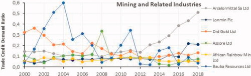
Figures 1 through 7 present companies' trade credit demand ratios (TCDR) defined as the quotient of annual total trade payables and annual total assets for the same year (Dary & Haruna, 2019).

Figure 1: TCDR for the retail industry

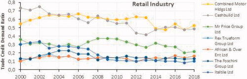
Figure 2: TCDR for the retail industry

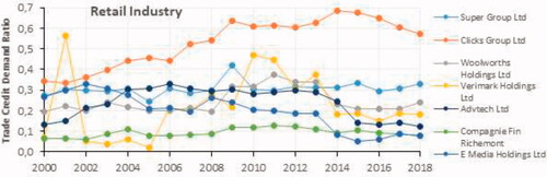
Figure 3: Miscellaneous producers

Figures 4: Mining and related industries

Figures 5: Mining and related industries

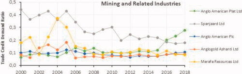
Figure 6: Technological hardware and equipment

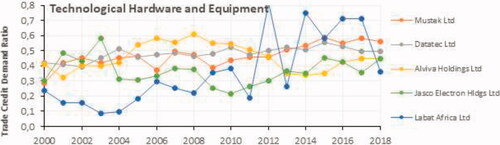
Figure 7: Food producers

References

- African Development Bank. (2014). Trade finance in Africa survey report. African Development Bank [Online] available: https://www.afdb.org/fileadmin/uploads/afdb/Documents/Publications/Trade_Finance_in_Africa_Survey_Report.pdf.
- Amiti, M. & Weinstein, D.E. (2011). ‘Exports and financial shocks’, The Quarterly Journal of Economics, 126(4): 1841–1877.
- Asian Development Bank. (2014). Asian development bank trade finance gap, growth and jobs survey. Asian Development Bank. [Online] available: https://www.adb.org/sites/default/files/publication/150811/adb-trade-finance-gap-growth.pdf.
- Asmundson, I., Dorsey, T.W., Khachatryan, A., Niculcea, I. & Saito, M. (2011). Trade and trade finance in the 2008-09 financial crisis. IMF Working Papers: 1–65.
- Asteriou, D. & Hall, S.G. (2015). Applied econometrics. Macmillan International Higher Education.
- Auboin, M. (2015). ‘Improving the availability of trade finance in low-income countries: An assessment of remaining gaps’, Oxford Review of Economic Policy, 31(3-4): 379–395.
- Auboin, M. (2016). Improving the availability of trade finance in developing countries: An assessment of the remaining gaps. Cesifo Working Paper.
- Auboin, M. & Engemann, M. 2014. ‘Testing the trade credit and trade link: Evidence from data on export credit insurance’, Review of World Economics, 150(4): 715–743.
- Bank of International Settlements. (2014). Trade finance: Developments and issues. Bank of International Settlements. [Online] available: https://www.bis.org/publ/cgfs50.pdf.
- Behrens, K., Corcos, G. & Mion, G. (2011). Trade crisis? What trade crisis? CEPR Discussion Paper no. 7956.
- Buckley, R.P., Arner, D.W. & Stanley, R.L. (2014). ‘Trade finance in East Asia: Potential responses to the shortfall’, Melb. J. Int'l L., 15: 109.
- CEIC. (2019). United States Nominal GDP. CEIC. [Online] available: https://www.ceicdata.com/en/indicator/united-states/nominal-gdp.
- Chauffour, J.P. & Farole, T. (2009). Trade finance in crisis: Market adjustment or market failure? The World Bank.
- Chicago Board Options Exchange. (2019). VIX index historical data. CBOE. [Online] available: http://www.cboe.com/products/vix-index-volatility/vix-options-and-futures/vix-index/vix-historical-data.
- Chicago Board Options Exchange. (2020). VIX index charts and data. Chicago Board Options Exchange. [Online] available: http://www.cboe.com/vix.
- Contessi, S. & De Nicola, F. (2012). The role of financing in international trade during good times and bad, In The regional economist. [Online] available: http://www.stlouisfed.org/publications/re/articles.
- Country Economy. (2020). South African credit rating history since 1980. [Online] available: https://countryeconomy.com/ratings/south-africa.
- Dary, S.K. & Haruna, I. (2019). Demand for and supply of trade credit in Africa. Department of economics & entrepreneurship development. Working Paper: WP/19/001
- Defever, F., Fischer, C. & Suedekum, J. (2016). ‘Relational contracts and supplier turn-over in the global economy’, Journal of International Economics, 103: 147–165.
- EViews. (2019). User’s guide: Advanced single equation analysis. Eviews. [Online] available: http://www.eviews.com/help/helpintro.html#page/content%2Frobustreg-Background.html%23ww133468
- Federal Reserve of St Louis. (2019). Bank capital to total asset ratio for United States. Federal Reserve of St Louis. [Online] available: https://fred.stlouisfed.org/series/DDSI03USA156NWDB.
- Federal Reserve of St Louis. (2020). Chicago Fed national financial condition index. Federal Reserve of St Louis. [Online] available: https://fred.stlouisfed.org/series/NFCI.
- Garralda, S., Maria, J. & Vasishtha, G. (2015). What drives bank-intermediated trade finance? Evidence from cross-country analysis. Bank of Canada Working Paper No. 2015-8.
- Holland, P.W. & Welsch, R.E. (1977). ‘Robust regression using iteratively reweighted least-squares’, Communications in Statistics-theory and Methods, 6(9): 813–827.
- Huber, P.J. (1973). ‘Robust regression: Asymptotics, conjectures and Monte Carlo’, The Annals of Statistics, 1(5): 799–821.
- International Chamber of Commerce. (2016). Rethinking trade and finance. International Chamber of Commerce. [Online] available: https://iccwbo.org/content/uploads/sites/3/2016/10/ICC-Global-Trade-and-Finance-Survey-2016.pdf.
- International Monetary Fund. (2009). A survey among banks assessing the current trade finance environment. International Monetary Fund. [Online] available: https://info.publicintelligence.net/IMFBAFTSurveyResults20090331.pdf.
- International Trade Centre. (2019). TradeMap. International Trade Centre. [Online] available: https://www.trademap.org/Index.aspx
- Kathuria, S. & Malouche, M. (2016). Strengthening competitiveness in Bangladesh – Thematic assessment: A diagnostic trade integration study. Washington DC: World Bank Publications.
- Kohler, A.S. & Saville, A. (2011). ‘Measuring the impact of trade finance on country trade flows: A South African perspective’, SA J of Economic and Management Sciences, 14(4): 436–448.
- Levchenko, A., Lewis, L. & Tesar, L. (2010). The collapse of international trade during the 2008-2009 crisis: In search of the smoking gun. NBER Working Paper no. 16006.
- Liston, D.P. & McNeil, L. 2013. ‘The impact of trade finance on international trade: Does financial development matter?’, Research in Business and Economics Journal, 8(1).
- Ljung, G.M. & Box, G.E. (1979). ‘The likelihood function of stationary autoregressive-moving average models’, Biometrika, 66(2): 265–270.
- Mathworks. (2019). Least squares fitting. Mathworks. [Online] available: https://www.mathworks.com/help/curvefit/least-squares-fitting.html.
- Paravisini, D., Rappoprt, V., Schnabl, P. & Wolfenzon, D. (2011). Dissecting the effect of credit supply on trade: Evidence from matched credit-export data. NBER Working Paper no. 16975
- Quantec. (2019). South Africa financial conditions index. Quantec. [Online] available: https://www.quantec.co.za/news/easydata-south-africa-financial-conditions-index/
- Ronci, M.M.V. (2004). Trade finance and trade flows: Panel data evidence from 10 crises. International Monetary Fund No 4-225.
- South African Reserve Bank. (2019). Historical exchange rates. South African Reserve Bank. [Online] available: https://www.resbank.co.za/Research/Rates/Pages/SelectedHistoricalExchangeAndInterestRates.aspx
- Trading Economics. (2019). South Africa – Capital to asset ratios. Trading Economics. [Online] available: https://tradingeconomics.com/south-africa/bank-capital-to-assets-ratio-percent-wb-data.html
- WTO. (2018). World trade report 2018. WTO. [Online] available: https://www.wto.org/english/res_e/publications_e/world_trade_report18_e.pdf.
- Yang, T., Gallagher, C.M. & McMahan, C.S. (2006). ‘A robust regression methodology via M-estimation’, Computer methods and programs in biomedicine, 82(1): 31.
- Zheng, G. & Yu, W. (2014). ‘Financial conditions index's construction and its application on financial monitoring and economic forecasting’, Procedia Computer Science, 31: 32–39.