Constraining 135 years of mass balance with historic structure-from-motion photogrammetry on Storglaciären, Sweden

ABSTRACT

Geodetic volume estimates of Storglaciären in Sweden suggest a 28% loss in total ice mass between 1910 and 2015. Terrestrial photographs from 1910 of Tarfala valley, where Storglaciären is situated, allow for an accurate reconstruction of the glacier's surface using Structure-from-Motion photogrammetry, which we used for past volume and mass estimations. The glacier's yearly mass balance gradient and net mass balance was also estimated back to 1880 using weather data from Karesuando, 170 km north-east of Storglaciären, through neural network regression. These combined reconstructions provide a continuous mass change series between the end of the Little Ice Age and 1946, when field data become available. The resultant reconstruction suggests a state close to equilibrium between 1880 and the 1910s, followed by drastic melt until the 1970s, constituting 76% of the 1910–2015 ice loss. More favourable conditions subsequently stabilized the mass balance until the late 1990s, after which Storglaciären started losing mass again. The 1910 reconstruction allows for a more accurate mass change series than previous estimates, and the methodology can be used on other glaciers where early photographic material exists.

KEYWORDS:

• structure-from-motion
• mass balance reconstruction
• climate change

1. Introduction

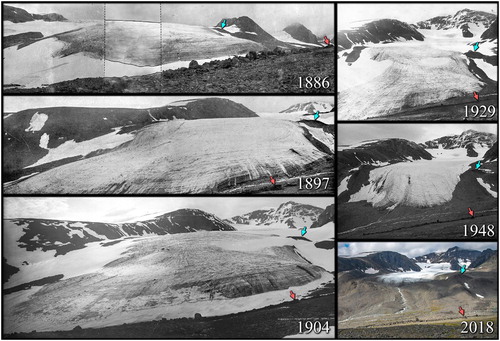
Sweden's glaciers have undergone an almost constant retreat since the early 1900s, after the end of the cold period known as the Little Ice Age (LIA). Glacier measurements in Sweden can be found as far back as the early 1800s, when most glaciers were still growing (Karlén 1973). Tarfala valley, in the northern Swedish mountain range, has been well documented since its first scientific visit in 1886, when Fredrik Svenonius photographed the valley's glaciers (Svenonius 1910). Since 1946, Tarfala Research Station has run an ongoing mass balance programme on Storglaciären, the largest glacier in Tarfala valley, where melt and snow accumulation is measured multiple times per year (Holmlund and Jansson 1999). Rabots glaciär, five kilometres west of Storglaciären, displayed clear signs of advancement in 1883 (Rabot 1898), and this local trend continued in Tarfala until the mid-1910s (Karlén 1973), after which Storglaciären retreated by almost 700 m (Figure 1). Between the beginning of the mass balance programme in 1946 and 2016, 45 out of 70 years have had a negative net balance, and a previous estimate suggests that Storglaciären lost about one-third of its mass since 1910 (Holmlund 1988).

Figure 1. The front of Storglaciären since 1886. The glacier reached its maximum late LIA extent in the 1910s, and has since then retreated. The photograph from 1886 was taken by Fredrik Svenonius, 1897 by Ali Nordgren and Albin Rönnholm, 1904 by Borg Mesch, 1929 by Ernst Herrmann, 1948 by Valter Schytt and 2018 by Erik S. Holmlund. Note the coloured arrows for visual aid, representing the same occurring details. A lateral moraine on the right-hand side (north) was visible in 1897, but was overridden in 1904, suggesting the moraine being present before the late LIA advance.

Comparing topographic maps and their constituent materials make precise volume measurements of glaciers possible, and many photographs have been taken in Tarfala valley for this purpose. In 1910, the geography student Fredrik Enquist visited Tarfala valley to make a photogrammetric map of the area, and took approximately 50 photographs of the valley. From these photographs, he produced a coarse map, which was complemented with photographs in 1922 by Arvid Odencrants, and were used for the first photogrammetrically derived map of the area (STF 1925), replacing an imprecise map made with material from 1877 to 1879 (Woxnerud 1951). The next photogrammetric surveys were conducted in 1946 and 1949 when the Swedish Air Force took nadir images over the valley. After this, Lantmäteriet (the Swedish mapping, cadastral, and land registration authority) has flown approximately once every decade. In addition, Lantmäteriet surveyed the valley and its surroundings in 2015 using Light Detection And Ranging (LIDAR) scanning. From these surveys, maps have been made, which have been used to estimate the change in volume for the glaciers in Tarfala valley (Holmlund 1988, 1996). More recent digital photogrammetry tools and better positioning systems, make higher accuracy elevation data possible, when compared to the usage of analogue maps in Tarfala valley (Koblet et al. 2010; Zemp et al. 2010). Volume changes have been calculated from the 1910–1922 map (Schytt et al. 1963), but its unreliable nature is reflected in these calculations, and its poor quality was one of the main arguments for performing the surveying flights in 1946 and 1949 to produce a better working map for Tarfala Research Station (Woxnerud 1951). Extracting elevation data with newer techniques from these older photographs is beneficial for reliably estimating the change in volume of Storglaciären, and the vast quantity of photographs from 1910 provides unprecedented potential for an accurate historic comparison.

Multiple studies have used proxy data to estimate the historic volume of Storglaciären, prior to the beginning of the mass balance programme in 1946. Schytt (1981) noted a strong correlation between the glacier's net mass balance gradient and summer temperature measured at Tarfala Research Station since 1946, strengthening the rationale for usage of temperature data to estimate its mass balance. Linderholm and Jansson (2007) used temperature derived from tree-ring data, as well as indices for the North Atlantic Oscillation, to estimate the mass balance of Storglaciären back to the 1500s, and suggested a decrease in cumulative net mass balance of about 12 metres water equivalent (m w.e.) for the period 1910–1946. Holmlund (1988) used summer temperature data from Karesuando, 170 km north east of Tarfala valley, in a linear regression analysis with Storglaciären's mass balance, and found a decrease of 22 m w.e. during the same time interval. Raper et al. (1996) used tree-ring derived temperature data and precipitation modelling, and found a decrease of about 20 m w.e., calculated from their volume estimate, using the conversions from this paper. Schytt (1947) used old maps and trim lines, and estimated a volume loss in the same period of 70 × 10⁶m³, or about 18 m w.e. However, the methodology is unclear, and the paper clearly highlights that the results are uncertain. This gives a spread between estimations of 12–22 m w.e., and the maps made by Enquist and Odencrants are not detailed or geometrically accurate enough to be used as a reference. Having a reliable estimate of the volume of Storglaciären in the early 1900s could provide a firm reference for models, strengthening their reliability further back in time, as well as providing a better view of the volume changes occurring over the last century.

The aim of this paper is to provide a continuous view of Storglaciären's mass change since 1880, using weather data to estimate the yearly changes until 1946, when field data become available, and constraining the cumulative estimated mass change to the calculated 1910 value. The weather data modelling is used to stretch further back in time than the first elevation models, to increase the temporal understanding of the glacier's variations. The inclusion of earlier photogrammetry-derived mass estimates gives the potential for a more reliable picture of Storglaciären's response to a changing climate. Few accurate mass reconstructions exist near the end of the LIA, but a large number of glaciers in Europe, and elsewhere, have a rich history of photographs from the last decade, and many of them have long field mass balance records. Using this information is important for understanding how and when the glaciers started retreating and thinning, in response to the post-LIA warming. The timing of glacier retreat is also vital for understanding and quantifying the anthropogenic impacts, as opposed to natural warming. We suggest that the methods of this paper can be applied to more glaciers, with suitable photographic material, to further quantify the effects of the warming after the end of the LIA.

1.1. Study area

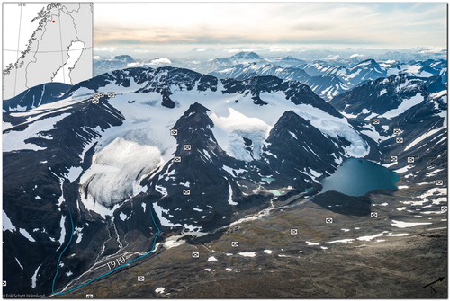
Storglaciären (67.90°N, 18.60°E) is a small valley glacier covering 3 km², with a current elevation range of 1140–1700 m a.s.l., but it has previously reached as low as 1020 m a.s.l. (Figure 2). The glacier is polythermal, with a 38 m thick cold surface layer over its temperate core as of 1989 (Holmlund and Eriksson 1989; Pettersson et al. 2003), but the cold layer is decreasing in thickness over time, probably due to a warming climate (Pettersson et al. 2003; Gusmeroli et al. 2012). The bed topography has been measured using ground penetrating radar, yielding depths of up to 250 m and a total volume of 306 × 10⁶m³ (Björnsson 1981), where the latter is used here as an absolute determination of the glacier's volume changes. Various weather parameters from Tarfala Research Station, a kilometre north east of Storglaciären, exist since 1945, measuring average summer and winter temperatures of +5.5°C and −8.9°C, respectively, as well as average summer and winter precipitation values of 350 mm w.e. and 600 mm w.e., respectively (Holmlund and Jansson 2002).

Figure 2. Estimated positions of the used 1910 terrestrial images, and the 1910 extent of Storglaciären (blue line). Also shown is the location of Tarfaladalen in Sweden. Photograph by Erik S. Holmlund, 17 August 2017.

The glaciers of Tarfala valley deposited their most distal moraines before the end of the LIA, ending around the 1910s (Karlén 1973; Karlén and Denton 1976), with most glaciers in the vicinity havinǵ multiple end moraines. Lichenometric dating of these moraines suggest multiple advances beyond the late LIA terminus positions since the late 1600s (Karlén 1973), and proxy data reconstructions also suggest larger glacier volumes over the few hundred years prior to the 1910s (Raper et al. 1996; Linderholm and Jansson 2007). Furthermore, Storglaciären advanced over an older lateral moraine between 1897 and 1904, a few years before its eventual retreat (Figure 1). Since this final advance, glaciers close to Tarfala valley lost mass considerably. Rabots glaciär, five kilometres west of Storglaciären, is estimated to have lost 30% of its volume during the period 1910–2003 based on area-volume relationships (Björnsson 1981; Brugger et al. 2005). Mikkaglaciären in Sarek, 65 km south west, experienced a 24% volume loss in the period 1960–2008 (Holmlund et al. 2016), and was considerably larger in the 1910s (Holmlund 1986). Kårsaglaciären, 50 km north, had a more extreme loss of 87% of its volume from 1926 to 2010 (Williams et al. 2016), illustrating the variation in volume change in the Swedish mountain range, and further motivating the use of more early 1900s data.

2. Methods

The methodology consists of three distinct steps for reconstructing the historic volume and mass of Storglaciären. Structure-from-Motion (SfM) photogrammetry (Koenderink and van Doorn 1991; Snavely et al. 2008; Westoby et al. 2012) can be used on the 1910 image series since the camera's internal distortion, or camera calibration, is unknown. This method allows for high accuracy reconstructions, with little or no image metadata, by estimating the camera calibration and photograph positions by the minimization of multi-variable cost functions, while using Ground Control Points (GCPs) to minimize internal distortion and to georeference the model. This process needs GCPs, which need to be acquired before the processing step. All SfM photogrammetric processing was performed in Agisoft PhotoScan 1.4.1, using global matching. Next, a relationship between average monthly temperature and total monthly precipitation data, compared to the glacier's mass balance, is constructed. This is constrained using the photogrammetric measurement of volume change from 1910, to provide a continuous series of mass change with lower errors.

2.1. Acquiring ground control points

In SfM photogrammetry, more ground control is needed than in traditional photogrammetry (James et al. 2017). When using SfM, a poor network of GCPs can result in a faulty camera calibration, thus introducing non-linear distortion within the image network, and thereby in the reconstructed terrain (e.g. Rosnell and Honkavaara 2012; Javernick et al. 2014; Girod et al. 2017). These errors are mitigated however, when dealing with an undulating terrain, or when the viewing direction of the image is not entirely vertical, or oblique (James and Robson 2014; Carrivick et al. 2016; Girod et al. 2018). Since the 1910 photographs are all oblique, and have a high overlap of distant features, common SfM-related issues such as doming, a deformation often seen with exclusively vertical images, should not be an issue here as long as the relative image alignment is correct.

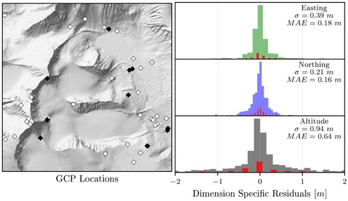
The collection of GCPs was done in PhotoScan, using well georeferenced aerial imagery, with an approximate ground sampling distance of 0.5 m, taken by Lantmäteriet in 2008. By identifying rocks and other features in the 2008 images, the absolute position of the feature can be determined and be used as a GCP. The feature needs to be visible and matched, or projected following the terminology of PhotoScan, in at least two images to get a three-dimensional position, but its accuracy will increase with an increasing amount of projections. A minimum of three projections was used, and each feature was projected in as many of the images as possible, with a maximum of six images. Aerially derived GCPs will be inferior to GCPs collected with a GNSS or Total Station in the field, in terms of horizontal and especially vertical accuracy, but points are easier and faster to collect, resulting in more ground control being available to use. A kind of precision estimate of these aerial GCPs can be acquired through iteratively varying which aerial images define the position of the GCP. By alternating between random pairs of images and noting the varying position of the GCP, its distribution of positions can be used to estimate the error of their placements (Figure 3). Here, 12 out of 95 available aerial GCPs could be identified in the 1910 images, with a horizontal Mean Absolute Error (MAE) of 0.24 m and vertical MAE of 0.64 m calculated from all 95 GCPs.

Figure 3. Errors of GCP placements depending on which aerial image pair was used, giving an estimate of the accuracy of the aerial GCP. Out of all 95 GCPs, extending beyond the confines of the map, 12 were used here and are highlighted in black. The histograms show the dimension-specific errors, as well as their standard deviations (σ) and Mean Absolute Errors (MAE), calculated from all 95 GCPs, with the used 12 shown in red.

2.2. SfM photogrammetry

Using modern photogrammetry in glaciology, parameters such as area, extent, shape and volume change can be accurately determined using images and ground control as input data. Here, terrestrial images from 1910 are used to extract the past volume and mass of Storglaciären. This can later be compared with reference 2 m gridded LIDAR data from 2015 (lantmateriet.se), to measure the changes in volume, by multiplying the mean vertical change with the 1910 area. The reference dataset has a reported vertical and horizontal accuracy of 5 and 25 cm, respectively. A standard ice density of 850 kg m⁻³ (Huss 2013) was used for volume to mass conversion, since there is no better estimation for Storglaciären.

Fredrik Enquist took around 120 positive glass plate photographs around the Kebnekaise massif during 22–26 July 1910. Out of these, 50 photographs portray Tarfala valley (Figure 2). The original glass plates were scanned using an Epson Perfection V700 Photo scanner at a resolution of 1200 dpi. Each of the glass plates have fiducial marks, making an estimation of their internal coordinate system possible (Figure 4). The fiducials come in pairs of two triangular features, and the left vertical and lower horizontal features were consistently used. With the fiducials marked in all of the images, their analogue positions were automatically estimated in PhotoScan using the scanning resolution as a real-world translation (1200 dpi). Masks were created around the fiducial marks, the image numbering and the sky of every image, to exclude these parts from the subsequent processing. By roughly masking out the sky, there is a lower risk of feature mismatching in the subsequent image alignment step, and the steps take less processing time by not having to process the entire image.

Alignment of the 1910 imagery needed manual tie points, as they would initially not automatically align correctly due to poor feature matches between them. In total there were 12 777 valid matches, but with only 1 147 occurring between more than two images. The reason for this shortcoming was probably due to noise and poor feature overlap between the images, and the feature matching algorithms did not provide enough matches for every image's relative orientation to be estimated. Manual tie points therefore needed to be added, to complement the automatic process (Figures 4 and 5). A total of 180 manual tie points were added of features throughout the valley, which were integral in aligning every image. Relying on manual tie points is questionable for estimating a good camera model, due to their inherently low quantity, leading to potential mismatches having a considerable effect on the outcome. Since every image shared a single model however, image pairs with many automatic matches were assumed to make up for the poorer images. The parameter errors compared to their magnitudes of the focal length (estimated to 181.72 ± 1.46 mm) and principal point estimation were 0.9%, while the radial distortion parameters had a 19% error. Parameter estimations preferably have errors at least a magnitude lower than themselves (Carrivick et al. 2016), or less than 10%, but consequences of these higher errors were not visible, and they were therefore not taken into further consideration.

Figure 4. Example of the photograph labelled E-271 from 1910 by Fredrik Enquist, looking towards Storglaciären (A). The image fiducials, exemplified in B, are used to align the images’ internal coordinate system. Manual tie points, using easily identified patterns, such as snow patches, had to be added for correct image alignment (C), where the automatic process failed.

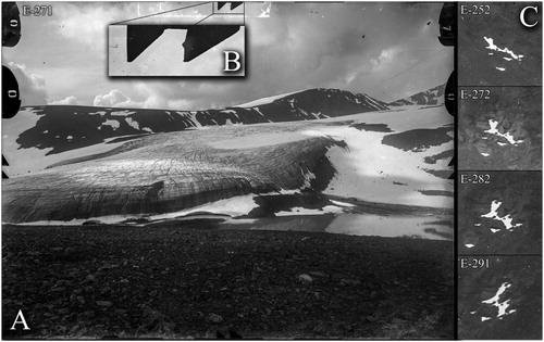
Figure 5. The reconstructed point cloud and manual tie points from 1910. Data gaps (no point within 50 m) in the lower half of the glacier are due to the lack of photographs picturing it, while the upper half is missing data due to lack of contrast in the snow. The two interpolation types are divided on the tongue, based on a topographic breaking point affecting the viewshed of the images.

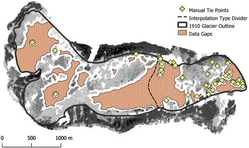
The dense point cloud reconstruction of the 1910 model was performed in PhotoScan using a quality of ‘Low’, and a depth filtering of ‘Moderate’, as these settings seemed to provide the most complete spatial coverage. The result was still extremely noisy, with approximately 80 000 out of 890 000 points remaining after cleaning the point cloud from noise. The points considered to be noise were clustered instead of being entirely random, and were therefore possible to manually remove from the point cloud. The result was a point cloud free of clustered erroneous points, and no further point filtering was considered necessary.

The coverage of the 1910 imagery was not sufficient for a complete reconstruction of the glacier's surface, with 34% of the surface having less than one point within a radius of 50 m (Figure 5). To fill the gaps in the model's surface, they were interpolated by adapting the shape of the 2015 surface to fit the 1910 data. The parts that were present in the 1910 model were initially compared with the 2015 points by measuring the distances between the surfaces. This was done using the M3C2 tool by Lague et al. (2013) in CloudCompare 2.9.1 with a projection and normal scale of 100 m. This means that it returns average distances within a radius of 50 m, normal to the slope at the point. The analysis provides a three-dimensional map of the surface-to-surface distance between the compared years, with 34% of the area still lacking data. These gaps were then spatially interpolated using linear interpolation, producing a complete surface change map over the whole glacier. The coordinates of the 2015 points were later lifted by its respective surface change distance, in the direction of the slope, raising them to fit the 1910 surface, while consequently linearly transforming its shape in the previous gaps to fill them seamlessly (Figure 6). Note that since linear interpolation was used for the surface change map, every part of the surface that already had data did not change, and the only changed parts are where gaps were present. This can be proven by comparing the interpolated surface with measured values where these exist. The comparison returned a mean offset of −0.02 m, and a standard deviation of 1.42 m, with the variance probably being due to the comparison of a noisy to a smoothed surface.

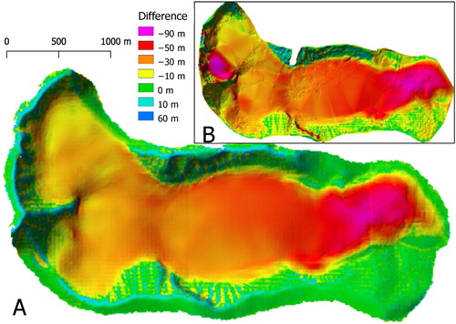
Figure 6. Height differences between 1910 and 2015 using the methodology of the study (A), and using simple linear interpolation (B).

Finally, since the aforementioned surface interpolation could only be performed as far as the glacier extended in 2015, an unscreened Poisson surface reconstruction, suitable for complex and noisy three-dimensional surface reconstructions, was performed on the 1910 front and in the surrounding terrain, while also disregarding noise as it smooths the original data (Kazhdan et al. 2006; Kazhdan and Hoppe 2013). This was problematic in areas close to the 1910 terminus, where points only existed on the glacier surface and not on the ground, due to unfavourable image perspectives, resulting in an overestimation of its extent. The overestimation was corrected for in the surface reconstruction, by using elevation data from 2015 outside of the glacier's 1910 terminus, to constrain the shape of its terminus.

This novel methodology of gap interpolation was initially preferred because it gave a credible visual appearance. Linear interpolation of gaps is a more established method (e.g. Kääb 2008; Pieczonka et al. 2013), and is argued to be one of the most suitable gap interpolation methods for measuring glacier change (McNabb et al. 2018). Both methods were therefore performed here in CloudCompare, and then compared. Figure 6 shows that the usage of linear interpolation in this case gives unreasonably high elevation differences in parts of the accumulation area, leading to larger resultant volume changes and much higher inherent errors (Table 1), calculated by the mean offset of all available periglacial surfaces (Figure 6). The gap interpolation method introduced in this study also contains possible errors, such as using the assumption of a similar glacier geometry between 1910 and 2015, which could be wrong, but with lower errors and a smoother shape, it appears favourable to the alternative.

Table 1. Results of the comparison between 1910 and 2015 surfaces, also seen in Figure 6.

Type	Glacier change (m)	Ground error (m)	Ground Stdev (m)	Volume change (m^3)
Raised surface	–30.35	1.02	7.39	–114.12 ± 5.83 × 10^6
Linear interpolation	–35.77	–9.66	13.96	–134.50 ± 36.32 × 10^6

Note: The glacier change values are the mean values within the 1910 extent. Ground error are the change values, or offsets, of the surfaces outside of the 1910 outline, and are used for the volume error estimates, shown together with their standard deviations.

Error in the 1910 reconstruction arises from multiple sources: the placement error of GCPs, error of the GCPs themselves, possible model distortions, the sparse nature of the point cloud, and the interpolation method applied in the study. The Root Mean Square Error (RMSE), the error measure automatically given by PhotoScan, of every GCP in the model was 3.28 m horizontally and 2.07 m vertically, averaged for the entire valley. This measure only encompasses the accuracy of the GCP placement, however, and reaches farther than the study area, so other measures are likely more representative for volume error over Storglaciären. For error in the volume reconstruction, the vertical offset of the surrounding ground was used instead, which was assumed to be relatively stable, together with a compensation for the presence of gaps in the surface. The error of these gaps are harder to assess, and the final error was therefore multiplied by a factor of $(1/1-0.34)\approx 1.52$ since 34% of the glacier surface was missing, leading to a resultant vertical error of 1.55 m. This was finally used to calculate the error of the raised surface volume estimate, seen in Table 1.

2.3. Mass balance regression

To estimate the mass balance of Storglaciären before the beginning of the mass balance programme, local weather data were correlated with a dataset of the measured mass balance gradients (Bolin 2018). A continuous series of monthly temperature and precipitation data (1880–2012) from Karesuando, 170 km north-east of Tarfala, was used for the analysis. Weather records also exist from Kiruna, Kvikkjokk and Riksgränsen, all relatively close to Tarfala, but were not used as they were either considered too short or were discontinuous. Since a glacier's response to weather depends on factors such as current size and geometry of the glacier (Cuffey and Paterson 2010), the net balance was not correlated directly to weather data. Instead, estimations of the mass balance gradient for each year were performed, which simply describes the accumulation or ablation as a function of altitude, and should therefore correlate better with weather. These mass balance gradients can then be applied to a varying glacier surface geometry, to reconstruct the glacier's net mass balance.

Storglaciären's net mass balance and June–August temperatures from Tarfala Research Station in 1965–2015 are moderately well linearly correlated (r = –0.72). Holmlund (1987) noted a higher June–August temperature correlation in Karesuando with the glacier's net balance (r = –0.80) measured from 1945 to 1986, but this correlation decreases when including data up to 2015 (r = –0.66). Because of this low correlation, the net mass balance of Storglaciären and temperature farther inland cannot be assumed to relate linearly, or a more difficult relationship is obstructing the comparison. More complex regression methods, or possibly more data, are therefore needed to accurately model Storglaciären's net mass balance.

To solve Storglaciären's apparent non-linear response between net mass balance and temperature, its mass balance gradient was instead modelled using supervised learning of a neural network. This type of programming structure can model intricate relations between variables, and has previously been used to estimate glacier mass change (Steiner et al. 2008; Moya Quiroga et al. 2013). A regular feed forward neural network takes one or multiple inputs and outputs, and passes it through a specified amount of hidden layers, wherein each layer contains a specified amount of neurons. These neurons carry out simple arithmetic operations, which affect the outcomes of its neighbouring connected neurons. The structure of a neural network is spider-web like, inspired by the connections of biological neurons, and allows an algorithm to learn its task, by fine tuning weights of its respective neurons to better fit the data. The model is trained using training data, iteratively modifying its weights to better predict it, and then tested using testing data. The testing data are put aside beforehand, usually constituting a random selection of around 20% of the total data, although this percentage can vary, to validate how the model performs on values it has never seen before. With the intricate structure of a neural network, complex interactions can be modelled, but understanding its structure becomes difficult, so the testing data exist to validate its accuracy.

Precipitation can have strong local variations, and is difficult to accurately measure. Therefore, the analysis was done both with and without using precipitation data, to evaluate its effect on the result. The mass balance gradient model was trained using measured data from 1946 to 2011, consisting of binned data in 20 m intervals from the lowest to the highest point on the glacier. For each separate interval and year, a comparison was made between weather data from the same mass balance year, the respective altitude, and the net balance of the interval in m w.e. The supplied weather data are thus from last year's October to the same year's September. The model is supplied with 25 predicting properties when including precipitation data, and 13 with only temperature data, consisting of twelve months of respective weather data values, and altitude. This produced 2 047 unique data points, whereby 20%, or 410 random points, were used strictly as testing data. The neural network was created and run using the open library Keras (Chollet 2015), on top of the TensorFlow library (Abadi et al. 2015), in Python. The parameters for the neural network were: three hidden layers with 30 neurons each, run over 2000 epochs, using Adadelta (Zeiler 2012) as the optimizer on default settings. After training the neural network, the comparison of predicted test data points to their respective targets in the test period of 1946–2011, provided a Mean Absolute Error (MAE) of 0.157 m using temperature and precipitation data, and 0.162 m when strictly using temperature data.

After having predicted the mass balance gradients, they were converted to changes in mass by multiplying them with 20 m equally binned area measurements, acquired from the photogrammetric models (Figure 7). These models only cover the specific years of 1910, and 2015, as well as 1959, 1969, 1980, 1990 and 1999 from Koblet et al. (2010), so interpolation had to be performed between the years, to provide a continuous series. For each separate elevation interval, the area bins were interpolated over time using quadratic spline interpolation, thus simulating the gradual temporal change in both surface area and geometry. As a consequence, retreat of the terminus was also simulated because the lower elevation area intervals eventually reach zero. By integrating these areas and mass balance bins with each other, the net balance in kilograms water equivalent (kg w.e.) is acquired for each year. The estimated cumulative mass change was finally corrected to fit the photogrammetric estimates of Koblet et al. (2010) and this study (Figure 8). Note that no constraint could be put on values before 1910, thus making them less reliable.

Figure 7. The area-altitude distribution in three of the seven elevation models (A), and the mass balance gradients, estimated from temperature data for the same years, calculated from a ±2 year average to display their general shapes (B). These are together used to later estimate the net mass balance for each year. Note that the estimated gradients shown in B can reach farther down than the actual glacier extends, since they are a direct result of the weather data modelling.

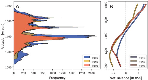
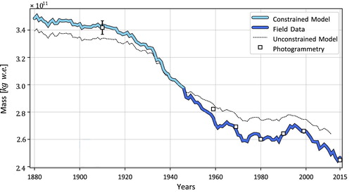
Figure 8. The constrained mass balance model from temperature data, shown with field data since 1946 and photogrammetry-derived estimates. The unconstrained mass change model is also shown (aligned with the 1946 mass), highlighting the importance of pinning points for cumulative measurements to be reliable. The photogrammetrical data from 1959 to 1999 are recalculated volume estimates from Koblet et al. (2010).

With the mass balance gradients for each distinct year successfully modelled, the Equilibrium Line Altitude (ELA) can be estimated by noting at which altitude the net mass balance is at zero. The zero mark was calculated using linear regression of the mass balance gradient, since a handful of years had a neutral mass balance at multiple altitudes. Analysing the ELA back in time can provide a better understanding of the glacier's fluctuations due to weather, and helps in validating the model to see if the values are reasonable.

3. Results

The photogrammetric and modelled mass changes show a lowering of 10.13 ± 1.32 m w.e. between 1910 and 1946, when comparing the photogrammetric mass estimate with the cumulative mass balance since 1946 (Figure 8). The areal extent decreased from 3.76 km² in 1910, measured in this study, to 3.30 km² in 1949 by Holmlund (1987). From 1880 to 1946, the model predicts 25 out of 66 years as having a positive mass balance, meaning that 50 of 135, or 37% of the years during 1880–2015 were positive. The mass change curve in Figure 8 displays a strong acceleration in melt in the 1930s, where Storglaciären lost 14.39 × 10⁹kg w.e. in 1910–1930 and 36.72 × 10⁹kg w.e. in 1930–1950. The curve further suggests that the changes between 1880 and the 1910s were relatively small, thus indicating a state close to equilibrium.

The strongest melt in the mass change curve of Figure 8 occurs between the 1930s and 1960s, with the beginning of this negative trend occurring in the early 1920s. The imagery from 1922 by Odencrants support this likely start of a melting trend, as almost no snow is present on top of Storglaciären, and other glaciers show tendencies of retreat. Between 1920 and 1970, 76% of the mass loss seen from 1910 to 2015 occurred while only constituting 48% of those years. This considerable melt, compared to the subsequent years, is also reflected in the retreat of the terminus, where it retreated approximately 370 m between 1929 and 1959 (Karlén 1973). The mass change of Storglaciären stabilized in the following years, even containing periods of increases in mass, and its mass was almost the same in 2001 as in 1970. Subsequent years have been strongly negative however, reminiscent of the 1930s to 1960s melt period.

The resultant MAE for the ELA estimates (Figure 9) was 40.89 m a.s.l. when comparing with measured data 1946–2011. The series in Figure 9 displays a generally lower ELA between 1880 and the 1930s, with occasional high values, and the ELA reaches comparable lows during the late 1970s and 1990s, corresponding with positive mass balance. The curve thus suggests similar conditions in the late 1800s to, for example, the 1990s. Worth noting however is that the glacier surface was higher in the beginning of the analysed time period, and a low ELA previously encompassed more of the upper glacier, as seen in Figure 7, leading to a higher potential accumulation.

Figure 9. The measured and estimated (temperature data only) net mass balance (A) together with the Equilibrium Line Altitude (B). C and D show the correlation between measured and estimated mass balance and ELA values in the period 1946–2011.

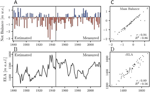
When comparing the mass balance models using temperature, with or without precipitation data, to the photogrammetric estimates, both mass balance models seem to underestimate the cumulative mass loss over the studied period. The inclusion of precipitation data also seems to adversely affect its performance, where this series gives an underestimation of 39.0%, while using only temperature data gives an underestimation of 16.5% Due to this, the model using only temperature was considered more reliable, and was consequently used for further analyses.

4. Discussion

The two weather models both predicted mass balance gradients well, with MAEs of 0.157 m using precipitation plus temperature, and 0.162 m using only temperature, when compared with measured testing data 1946–2011. When applying these gradients to the glacier surface however, both of the cumulative curves underestimated Storglaciären's mass loss when comparing with the photogrammetrically derived values. Smaller effects on the mass balance record, such as internal accumulation, are not accounted for in the provided mass balance data, but these are considered neglectable in the case of Storglaciären (Zemp et al. 2010). This suggests the models either underestimating ablation, accumulation, or both.

Since the gradients were so well correlated with their testing data, this underestimation is likely due to the way mass change was calculated. The elevation models’ Z errors vary between 1.02 and 4.08 m, and this small possible offset could adversely affect the area binning process, thus giving the glacier wrong proportions. Furthermore, the subsequent bin interpolation between the photogrammetric years could also misrepresent these area proportions. This model underestimation is however visible over the whole series, even in tightly constrained intervals such as 1990–1999 (Figure 8), making the area interpolation cause less likely. One possible source of the models’ underestimation of mass variation over time might be due to certain extreme years being poorly modelled, therefore continually accumulating error over time. This might explain the obvious outliers seen in Figure 9, in the correlation between measured and estimated mass balance values from 1946 to 2011. These outliers are a plausible cause of the cumulative errors, since the same area curve was used in the measured and estimated series (Figure 8), and their yearly values in m w.e. is the only thing differing the two weather models. Such an interpretation would suggest extreme years having a considerable long-term impact on the glacier's mass balance.

The shape of the mass curve before 1910, more or less suggests a state of equilibrium between 1880 and the 1910s (Figure 8). This is challenged by earlier observations from 1897 and onward, where an advance of the terminus is evident, thus suggesting a positive net balance. A reason for this possible error might be in the shortcoming of the area binning, used for calculating the mass balance, where no measurement exists before 1910, and the previous years were therefore fixed to the 1910 surface. As a consequence, the size of the terminus was overestimated which would subsequently overestimate the ablation, and therefore might inhibit any estimated positive mass change before 1910. The curve nevertheless suggests a state close to equilibrium, which is not unlikely since the changes observed before 1910 are relatively small.

The majority of the strong 1920s to early 1970s mass loss (Figures 8 and 9), likely occurred in the lower part of the glacier, seen by the front's fast retreat and thinning (Figure 1). From 1900 to 1920, the mean June–August temperature in Karesuando was 9.88°C, while it rose to 11.63°C for the period 1930–1950. The main body of Storglaciären is overdeepened (Björnsson 1981) with a high ice flow velocity, and a decreasing velocity nearing its front due to its polythermal nature (Hooke et al. 1989). This overdeepening ends in a small bedrock riegel, which might have constricted the flow of ice, and therefore could have played a large role in the glacier's past dynamics. The mass loss coincidentally started to stabilize as the terminus was nearing this riegel, highlighting the role of the glacier's basal topography on the retreat of its terminus. The thinning of a polythermal glacier can also make its tongue colder and thus slower (Delcourt et al. 2013), possibly further constricting the flow of ice past the riegel, which might have hindered the lowermost parts of the glacier from being replenished in the 1900s. The glacier's basal topography, together with a warming climate, are therefore both likely causes of its strong melt in the first half of the 1900s.

The inclusion of precipitation data in the model proved to have an adverse effect on its outcome, shown by the large cumulative mass loss underestimation, yet the errors in the testing data were 3% lower than when precipitation data was not used. One possible explanation of this is that the quality of the precipitation data might vary over the years, thus potentially providing a good correlation after 1946 but being erroneous before. Another possible explanation is due to the nature of the model's neural network itself, where poor data can adversely affect the prediction with no easy way of detecting it. In a scenario that there is no correlation between precipitation in Karesuando and net balance on Storglaciären, their respective weights should theoretically tend towards zero and would not affect the final prediction. Error might however induce false correlations between the two, resulting in weights above zero, thus impairing the performance of the model. Furthermore, the random choice of which data will become testing data should not affect the outcome, if the errors in the data are entirely stochastic and the sample size is large enough. If these two criteria are not filled however, the choice of testing data will have an effect on the resultant errors, and multiple attempts with the same input data can produce slightly different outcomes each time. Therefore, even if removing precipitation provided an increase in error by 3%, this might be entirely due to the random choice of testing data. The model's stochastic nature, coupled with possible erroneous correlations in the precipitation data, could therefore provide a poorer model yet with slightly lower errors.

The unconstrained mass change curve in Figure 8 shows that the estimated curves (with or without precipitation data) underestimate the periods of positive mass balance seen in the 1960s, late 1970s and 1990s. These periods of positive mass balance were likely due to the increase in winter precipitation seen around Tarfala at the same time, and is also suggested by the low ELAs (Figure 9). More snow is a reasonable explanation for why only using temperature to estimate Storglaciären's mass balance can give faulty values during these positive periods, as this is evidently not reflected in the temperature series from Karesuando. The inclusion of precipitation from Karesuando in the modelling did on the other hand not change this behaviour, shown by these curves being equally poor at estimating positive mass balances. This could either suggest that an unknown factor is negatively affecting the estimation, or that precipitation in Karesuando simply does not correlate well enough with the mass balance of Storglaciären.

The weather station in Riksgränsen, 61 km north of Tarfala, is much closer and geographically similar than Karesuando which is located in a more continental setting, and estimations including precipitation from Riksgränsen consequently showed a better fit when encountering positive mass balance periods. This estimation was not used however, as data from the whole year are only available since 1905, and many years in between are missing in the series. The data gaps reduced the amount of available data to train the model, and would shift the cumulative mass balance calculation, so data Karesuando was preferred. The better ability to model positive mass balance with Riksgränsen data nonetheless strengthens the suggestion that precipitation in Karesuando is too different to use in Tarfala, as was similarly found by Holmlund (1988).

5. Conclusions

The aim of the study was to provide a reliable estimate of the historic changes in mass of Storglaciären, using weather data to estimate the varying mass balance gradients, to calculate changes in mass. Furthermore, photogrammetric mass estimates with lower and more easily quantifiable errors, were used to constrain the series. The results showed that mass balance gradients can be successfully modelled using temperature data 170 km away from the site, but cumulative mass estimates gradually lose their accuracy without photogrammetric constraints. By including constraints however, accuracy and continuity are combined to provide a reliable series.

By comparing the photogrammetric estimates of Storglaciären between 1910 and 2015, the analysis shows a loss of 97.01 ± 4.96 × 10⁹kg w.e., or about 28% of its 1910 mass. From 1910 to 1946, the constrained series suggests a loss of 10.13 ± 1.32 m w.e. or 42.98 × 10⁹kg. The resultant mass series also suggests a state close to equilibrium between 1880 and the 1910s, although this period is less reliable as it cannot be constrained with photogrammetric estimates. Subsequently, a considerable period of melt occurred until around the 1970s when the mass variation stabilized over the 1980s and 1990s. The strong melt period of 1920–1970 constitutes 48% of the years, but makes up 76% of the mass loss seen in the period of 1910–2015. This melt period is likely a result of both increases in temperature, and of unfavourable basal topography conditions which facilitated retreat. The melt period was followed by a decrease in melt and even periods of positive mass balance, but a negative trend has been continuing since the 2000s, with no other apparent explanation than increasing temperature.

Acknowledgements

We would like to thank the Stockholm University, and the reviewers for helpful improvements to the manuscript. Thanks also to all the people who have conducted the field mass balance measurements from Tarfala Research Station over the years. This paper is based on a Bachelor-degree thesis (DOI:10.13140/RG.2.2.24483.91681).

Disclosure statement

No potential conflict of interest was reported by the authors.

Correction Statement

This article has been republished with minor changes. These changes do not impact the academic content of the article.

Notes on contributors

Erik S. Holmlund was born in 1996. Erik finished his bachelor of science in Physical Geography at Stockholm University in the spring 2018. He is now following a Master program in Quaternary Geology at the University Centre in Svalbard. He is specialized in the use of photogrammetry in geoscience.

Per Holmlund was born in 1956, is Professor in Glaciology at Stockholm University since 1999, obtained PhD in 1989 and was associate professor in 1992. Holmlund's research has been linked to climatic issues but covers glacial hydrology, radar soundings, photogrammetry, ice sheet modelling and other aspects. Holmlund's field sites have been in Swedish Lapland, Svalbard, Antarctica, Chile, the Arctic Sea and ice caves in Norway and Romania. Holmlund is Director of Tarfala Research station from 1996 to 2004, is Swedish delegate in WGMS, IUGG-IACS, and was formerly a glaciological representative of SCAR and IASC. In addition to scientific writing Holmlund is also fond of popular science writing and is author to books and chapters in books.

References

- Abadi M, Agarwal A, Barham P, Brevdo E, Chen Z, Citro C, Corrado GS, Davis A, Dean J, Devin M, et al. 2015. TensorFlow: large-scale machine learning on heterogeneous systems. www.tensorflow.org/.
- Björnsson H. 1981. Radio-echo sounding maps of Storglaciären, Isfallsglaciären and Rabots glaciär, northern Sweden. Geogr Ann A. 63:225. DOI:10.2307/520835 doi: 10.1080/04353676.1981.11880037
- Bolin. 2018. The Bolin Centre. https://bolin.su.se/data/tarfala/Storglaciären.php.
- Brugger KA, Refsnider KA, Whitehill MF. 2005. Variation in glacier length and ice volume of Rabots glaciär, Sweden, in response to climate change, 1910–2003. Ann Glaciol. 42:180–188. DOI:10.3189/172756405781813014.
- Carrivick JL, Smith MW, Quincey DJ. 2016. Structure from motion in the geosciences. 1st ed. New analytical methods in earth and environmental science. Chichester: Wiley Blackwell. OCLC: 910772463.
- Chollet F. 2015. Keras, the Python deep learning library. www.keras.io.
- Cuffey K, Paterson WSB. 2010. The physics of glaciers. 4th ed. Burlington, MA: Butterworth-Heinemann/Elsevier. OCLC: ocn488732494.
- Delcourt C, Van Liefferinge B, Nolan M, Pattyn F. 2013. The climate memory of an Arctic polythermal glacier. J Glaciol. 59:1084–1092. DOI:10.3189/2013JoG12J109.
- Girod L, Nielsen NI, Couderette F, Nuth C, Kääb A. 2018. Precise DEM extraction from Svalbard using 1936 high oblique imagery. Geosci Instrum Methods Data Syst. 7:277–288. DOI:10.5194/gi-7-277-2018.
- Girod L, Nuth C, Kääb A, Etzelmüller B, Kohler J. 2017. Terrain changes from images acquired on opportunistic flights by SfM photogrammetry. Cryosphere. 11:827–840. DOI:10.5194/tc-11827-2017 doi: 10.5194/tc-11-827-2017
- Gusmeroli A, Jansson P, Pettersson R, Murray T. 2012. Twenty years of cold surface layer thinning at Storglaciären, sub-Arctic Sweden, 1989–2009. J Glaciol. 58:3–10. DOI:10.3189/2012JoG11J018.
- Holmlund P. 1986. Mikkaglaciären: bed topography and response to 20th century climate change. Geogr Ann A. 68:291. DOI:10.2307/521522.
- Holmlund P. 1987. Mass balance of Storglaciären during the 20th century. Geogr Ann A. 69:439. DOI:10.2307/521357.
- Holmlund P. 1988. Studies of the drainage and the response to climatic change of Mikkaglaciären and Storglaciären. Number 220 in Meddelanden från Naturgeografiska Institutionen vid Stockholms Universitet. A. Stockholm: Univ. OCLC: 46136236.
- Holmlund P. 1996. Maps of Storglaciären and their use in glacier monitoring studies. Geogr Ann A. 78:193. DOI:10.2307/520981 doi: 10.1080/04353676.1996.11880456
- Holmlund P, Clason C, Blomdahl K. 2016. The effect of a glaciation on East Central Sweden: case studies on present glaciers and analyses of landform data. Technical Report 2016:21. Strålsäkerhetsmyndigheten.
- Holmlund P, Eriksson M. 1989. The cold surface layer on Storglaciären. Geogr Ann A. 71:241. DOI:10.2307/521394.
- Holmlund P, Jansson P. 1999. The Tarfala mass balance programme. Geogr Ann A. 81:621–631. DOI:10.1111/1468-0459.00090 doi: 10.1111/j.0435-3676.1999.00090.x
- Holmlund P, Jansson P. 2002. Glaciological research at Tarfala Research Station. Stockholm: Stockholm University.
- Hooke RL, Calla P, Holmlund P, Nilsson M, Stroeven A. 1989. A 3 year record of Seasonal variations in surface velocity, Storglaciären, Sweden. J Glaciol. 35:235–247. DOI:10.3189/S0022143000004561.
- Huss M. 2013. Density assumptions for converting geodetic glacier volume change to mass change. Cryosphere. 7:877–887. DOI:10.5194/tc-7-877-2013.
- James MR, Robson S. 2014. Mitigating systematic error in topographic models derived from UAV and ground-based image networks. Earth Surf Processes Landforms. 39:1413–1420. DOI:10.1002/esp.3609.
- James MR, Robson S, d’Oleire Oltmanns S, Niethammer U. 2017. Optimising UAV topographic surveys processed with structure-from-motion: ground control quality, quantity and bundle adjustment. Geomorphology. 280:51–66. DOI:10.1016/j.geomorph.2016.11.021.
- Javernick L, Brasington J, Caruso B. 2014. Modeling the topography of shallow braided rivers using structure-from-motion photogrammetry. Geomorphology. 213:166–182. DOI:10.1016/j.geomorph.2014.01.006.
- Kääb A. 2008. Glacier volume changes using ASTER satellite stereo and ICESat GLAS laser altimetry. A test study on Edgeøya, Eastern Svalbard. IEEE Trans Geosci Remote Sens. 46:2823–2830. DOI:10.1109/TGRS.2008.2000627.
- Karlén W. 1973. Holocene glacier and climatic variations, Kebnekaise mountains, Swedish Lapland. Geogr Ann A. 55:29. DOI:10.2307/520485 doi: 10.1080/04353676.1973.11879879
- Karlén W, Denton GH. 1976. Holocene glacial variations in Sarek National Park, northern Sweden. Boreas. 5:25–56. DOI:10.1111/j.1502-3885.1976.tb00329.x.
- Kazhdan M, Bolitho M, Hoppe H. 2006. Poisson surface reconstruction. Proceedings of the Fourth Eurographics Symposium on Geometry Processing. Eurographics Association. p. 61–70.
- Kazhdan M, Hoppe H. 2013. Screened Poisson surface reconstruction. ACM Trans Graph. 32:1–13. DOI:10.1145/2487228.2487237.
- Koblet T, Gartner-Roer I, Zemp M, Jansson P, Thee P, Haeberli W, Holmlund P. 2010. Reanalysis of multi-temporal aerial images of Storglaciären, Sweden (1959–99) – Part 1: determination of length, area, and volume changes. Cryosphere. 4:333–343. DOI:10.5194/tc-4-333-2010.
- Koenderink JJ, van Doorn AJ. 1991. Affine structure from motion. J Opt Soc Am A. 8:377. DOI:10.1364/JOSAA.8.000377.
- Lague D, Brodu N, Leroux J. 2013. Accurate 3d comparison of complex topography with terrestrial laser scanner: application to the Rangitikei canyon (N-Z). ISPRS J Photogramm Remote Sens. 82:10–26. DOI:10.1016/j.isprsjprs.2013.04.009.
- Linderholm HW, Jansson P. 2007. Proxy data reconstructions of the Storglaciären (Sweden) mass- balance record back to AD 1500 on annual to decadal timescales. Ann Glaciol. 46:261–267. DOI:10.3189/172756407782871404.
- McNabb R, Nuth C, Kääb A, Girod L. 2018. Sensitivity of geodetic glacier mass balance estimation to DEM void interpolation. Cryosphere Discuss. 1–29. DOI:10.5194/tc-2018-175.
- Moya Quiroga V, Mano A, Asaoka Y, Kure S, Udo K, Mendoza J. 2013. Snow glacier melt estimation in tropical Andean glaciers using artificial neural networks. Hydrol Earth Syst Sci. 17:1265–1280. DOI:10.5194/hess-17-1265-2013.
- Pettersson R, Jansson P, Holmlund P. 2003. Cold surface layer thinning on Storglaciären, Sweden, observed by repeated ground penetrating radar surveys. J Geophys Res: Earth Surf. 108. DOI:10.1029/2003JF000024 doi: 10.1029/2001JC001164
- Pieczonka T, Bolch T, Junfeng W, Shiyin L. 2013. Heterogeneous mass loss of glaciers in the AksuTarim Catchment (Central Tien Shan) revealed by 1976 KH-9 Hexagon and 2009 SPOT-5 stereo imagery. Remote Sens Environ. 130:233–244. DOI:10.1016/j.rse.2012.11.020.
- Rabot C. 1898. Au Cap Nord: Itineraires En Norvege, Suede, Finlande. Librarie Hachette et C:ie, Paris.
- Raper SCB, Briffa KR, Wigley TML. 1996. Glacier change in northern Sweden from AD 500: a simple geometric model of Storglaciären. J Glaciol. 42:341–351. DOI:10.3189/S0022143000004196 doi: 10.1017/S0022143000004196
- Rosnell T, Honkavaara E. 2012. Point cloud generation from aerial image data acquired by a quadrocopter type micro unmanned aerial vehicle and a digital still camera. Sensors. 12:453–480. DOI:10.3390/s120100453.
- Schytt V. 1947. Glaciologiska arbeten i Kebnekajse. Ymer. 67:18–42.
- Schytt V. 1981. The Net mass balance of Storglaciären, Kebnekaise, Sweden, related to the height of the equilibrium line and to the height of the 500 mb surface. Geogr Ann A. 63:219–223. DOI:10.1080/04353676.1981.11880036.
- Schytt V, Jonsson S, Cederstrand P. 1963. Notes on glaciological activities in Kebnekaise, Sweden – 1963. Geogr Ann. 45:292. DOI:10.2307/520124.
- Snavely N, Seitz SM, Szeliski R. 2008. Modeling the world from internet photo collections. Int J Comput Vision. 80:189–210. DOI:10.1007/s11263-007-0107-3.
- Steiner D, Pauling A, Nussbaumer SU, Nesje A, Luterbacher J, Wanner H, Zumbuhl HJ. 2008. Sensitivity of European glaciers to precipitation and temperature – two case studies. Clim Change. 90:413–441. DOI:10.1007/s10584-008-9393-1.
- STF. 1925. Svenska Turistforeningens Atlas over Sverige.
- Svenonius F. 1910. Die Gletscher Schwedens Im Jahre 1908. SGU Ca. 5:1–54.
- Westoby M, Brasington J, Glasser N, Hambrey M, Reynolds J. 2012. ‘Structure-from-motion’ photogrammetry: a low-cost, effective tool for geoscience applications. Geomorphology. 179:300–314. DOI:10.1016/j.geomorph.2012.08.021.
- Williams CN, Carrivick JL, Evans AJ, Rippin DM. 2016. Quantifying uncertainty in using multiple datasets to determine spatiotemporal ice mass loss over 101 years at Kårsaglaciären, sub-Arctic Sweden. Geogr Ann A. 98:61–79. DOI:10.1111/geoa.12123.
- Woxnerud E. 1951. Kartografiska arbeten i Kebnekajse. Geogr Ann. 33:121–130.
- Zeiler MD. 2012. ADADELTA: an adaptive learning rate method. CoRR abs/1212.5701.
- Zemp M, Jansson P, Holmlund P, Gartner-Roer I, Koblet T, Thee P, Haeberli W. 2010. Reanalysis of multi-temporal aerial images of Storglaciären, Sweden (1959–99) – Part 2: comparison of glaciological and volumetric mass balances. Cryosphere. 4:345–357. DOI:10.5194/tc-4-345-2010.