Isolating incident and reflected wave spectra in the presence of current

ABSTRACT

It is vital for a variety of coastal and ocean engineering problems to understand the reflection characteristics of structures and devices. Various methods have been developed for wave-only cases, yet none have been demonstrated for wave–current conditions present in both the laboratory and real sea environments. A simple method to isolate wave reflections in collinear current is presented in this article, utilizing an established frequency-domain least-squares approach with a modified dispersion relation. The method has been tested numerically, before being applied to experimental data obtained at the FloWave Ocean Energy Research Facility. Typical wave spectra are generated in currents ranging from −0.3 m/s to 0.3 m/s. Results obtained demonstrate the method effectiveness whilst verifying that the assumptions are valid. The development of this method should enable reflection analysis to be performed for wave–current conditions with improved accuracy and greater confidence.

KEYWORDS:

• Wave-Current Interactions
• Wave Reflection Analysis
• Tank Testing
• Wave Action

1. Introduction

Wave reflections exist due to wave field interaction with natural coastline, or man-made structures such as breakwaters and harbors, as assessed in Dickson, Herbers, and Thornton (1995), Chen, Tsai, and Chiu (2006) and others. For coastal engineering problems, it is vital to characterize the reflection from such structures to assess the likely influence on the surrounding conditions. This includes the potential for adverse effects on shipping due to the creation of potentially dangerous standing waves, or increased sediment scour compromising structural stability of the structure itself (Zanuttigh and van der Meer (2008) and Zanuttigh, Formentin, and Briganti (2013)). It is also important to characterize reflection or radiation when carrying out scaled laboratory tests. The characterization of reflections from scale models such as breakwaters or wave energy converters can be achieved prior to full-scale deployment. Knowledge of reflection coefficients can also be highly useful when calibrating sea states prior to model testing, enabling validated incident wave spectra to be specified without influence from side-wall or beach reflections.

There exists a variety of methods to isolate the incident and reflected wave spectra. Many of these approaches, such as the 1D methods presented in Mansard and Funke (1980) and Zelt and Skjelbreia (1992), are essentially extensions of the frequency-domain approach first presented in Goda and Suzuki (1976). Others, such as Frigaard and Brorsen (1995), are solved in the time domain. In all of these approaches, the dispersion relation is assumed to hold. However, in combined wave–current scenarios, this is no longer a valid assumption and, as such, implementing these methods without suitable adaptation leads to errors.

In this article, we describe and demonstrate a methodology for isolating incident and reflected wave spectra in collinear combined wave–current conditions. Section 2 presents a simple extension to the Zelt and Skjelbreia (1992) reflection analysis approach, using a theoretical modified dispersion relation to account for the presence of current [Jonsson (1990)]. In Section 3, the method is demonstrated using a numerical simulation and errors incurred from omitting the wavelength change in current are highlighted. In Section 4, experimental results are obtained from the FloWave Ocean Energy Research Facility, a combined wave–current test basin. Experiments allow for the method’s assumptions to be properly tested, namely that the modified dispersion is valid and the flow in the measurement region can be approximated as steady, uniform, and irrotational. The standard assumptions present in linear wave theory also apply. The presented approach is then used to isolate incident and reflected wave spectra for the FloWave basin, using a variety of typical sea states in a range of collinear current fields. Discussion introduces a wave-action-based reflection coefficient to enable fairer comparison of reflection and absorption characteristics in different current conditions.

2. Resolving wave reflections in current

In this section, the effect current has on wave properties is detailed. This knowledge is used to help inform a reflection analysis procedure for when current is present. Section 2.1 details the effect current has on wave shape and properties, whilst Section 2.2 shows how the knowledge of the transformed wavenumbers in current are used to help isolate incident and reflected wave spectra.

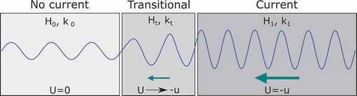
Figure 1. Diagram showing wave propagating from region of no current to a region with current. Change in wave height and wavelength (wavenumber) due to interaction with current field is indicated. Example is shown with opposing current (negative U) where wave height increases and wavelength decreases.

2.1. The effect of current on wave properties

Current alters the form of the waves, and as such the assumptions made in typical reflection analysis procedures are no longer valid. In particular, the wavelengths are modified and are no longer related to frequency through the standard dispersion relation, Equation (1). A modified relationship described in Jonsson (1990), Equation (2), is used instead. In the following equations, subscripts and refer to regions with and without current, respectively (see Figure 1) and refers to values relative to the current field, i.e., assuming a frame of reference moving at the same velocity as the current.

(1)

(2)

where is the angular frequency [rad s], is the wavenumber [m], is the current velocity [ms], and is acceleration due to gravity [ms]

In Equation (2) is defined as positive for waves in a following current and negative for the opposing case. When both incident and reflected waves (from a device or structure) coexist with the current field, they will have different wavenumbers. Wavelengths are shortened in opposing current and lengthened when following, which is accompanied by a change in wave height, or component wave amplitude, . This change in both wave height and wavelength is represented in Figure 1, where wave transformation is indicated for waves opposing current, and the regions of no current and current are highlighted. Conservation of wave action can be used to infer the expected wave height transformation, shown in Equations. (3) to (5) [Jonsson (1990);Smith (1997)].

(3)

(4)

where is the group velocity of a wave component in zero current and is the group velocity in current, assuming a reference moving at the same velocity as the current.

(5)

2.2. Isolating incident and reflected wave spectra in the presence of current

Assuming that the theoretical alteration to wavelength in the presence of current is valid (Section 2.1), it is then possible to isolate incident and reflected wave spectra using a linear array of wave gauges. The method presented here is essentially a modified version on the Zelt and Skjelbreia (1992) formulation, chosen as it can be solved for with an arbitrary number of wave gauges. The solutions presented in this article are found numerically and are found in the frequency domain utilizing a least-squares approach to find the best solution to the over-resolved problem (if ).

The surface elevation for a one-dimensional sea state consisting of incident and reflected wave components (from a structure or device), in the presence of collinear current, is described in Equation (6). Assuming linear wave theory, this can be described as a Fourier sum of incident and reflected wave components:

(6)

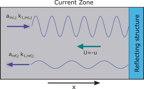
where inc refers to incident waves, ref reflected waves, and refers to the current altered wavenumber of the j^th component of the incident wave spectrum, calculated from Equation (2). Figure 2 depicts this combined wave–current field with reflection for a given frequency component. This highlights that in the measurement area (current zone), for every frequency component, there are two wavenumbers which are a function of , and (Equation. (2)), and there are two complex amplitudes which are unknown and to be resolved.

Figure 2. Wave field in the measurement (current) zone is made up of incident and reflected components from a structure. In the diagram, the reflecting structure is shown inside the current zone but could equally be in a region of still water. The figure highlights that for a given frequency component, j, there exists two wavenumbers and amplitudes for each frequency. This example depicts a case with opposing current (negative U) where wavelength decreases for incident and increases for reflected wave components.

The theoretical Fourier coefficients, , at wave gauge can be expressed as:

(7)

To resolve the incident and reflected spectra in an overdetermined system, the discrepancy between the measured, , and theoretical Fourier coefficients, , is minimized. This is described in Equation (8) for each frequency component and every wave gauge.

(8)

The merit function, , to minimize is based on the weighted sum of square errors across all wave gauges:

(9)

The minimum of Equation (9) occurs when Equations (10) and (11) hold:

(10)

(11)

In Zelt and Skjelbreia (1992), the equivalent solutions to Equations (10) and (11) are found analytically. In this article, these equations are solved for numerically using a Newton–Raphson iteration. The weights, , have been chosen to match those presented in Zelt and Skjelbreia (1992) to allow fair comparison; however, those suggested in Draycott et al. (2016) could equally be used.

3. Numerical simulation

A numerical simulation has been carried out to verify the method solution procedure and assess the errors incurred from omitting the wavenumber transformation. A JONSWAP [Hasselmann et al. (1973)] spectrum has been used with a significant wave height () of 3 m, a peak period () of 14 s, and a peak enhancement factor () of 3.3. This sea state was chosen to be narrow banded with a low peak period to avoid simulating wave blocking (see Moreira and Peregrine (2012)) in high-opposing current scenarios.

The sea state has been simulated using linear wave theory in current velocities ranging from −1.5 m/s to 1.5 m/s with a frequency-independent reflection coefficient, of 0.3 (relative to amplitudes unmodified by current). Modifications to incident and reflected spectral shape and wavenumber have been accounted for using Equation (2) and Equation. (5), noting that energy density, . Using MATLAB, an inverse fast Fourier transform (IFFT) applied to Equation (7) provides the total time series at chosen positions. These time series are used as inputs to the reflection analysis function. Random phases incorporated into the complex values and provide more realistic inclusion of the incident and reflected components. These have been simulated over a hypothetical nine-wave gauge array, with values chosen to be a full scale equivalent of the array shown in Figure 6 and used for the experimental testing.

Figure 3. Isolation of incident and reflected spectra, incorporating wavelength change due to current.

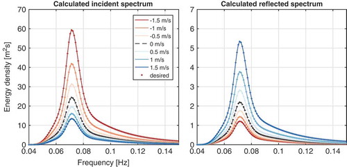
Figure 4. Isolation of incident and reflected spectra, omitting wavelength change due to current.

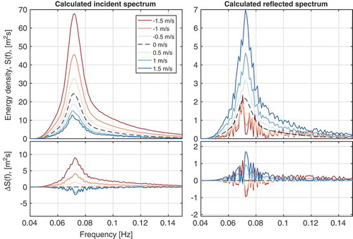
Figure 5. The FloWave Ocean Energy Research Facility. Image courtesy of Mr Donald Noble, FloWave.

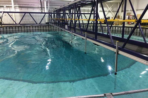
Figure 6. Reflection array based on eighth-order Golomb ruler.

The modified reflection method presented in Section 2, along with the unmodified equivalent, have been applied to the simulated time series with estimates of incident and reflected spectra shown in Figures 3 and 4. As expected due to being an idealized simulation, when incorporating the wavelength change, the incident and reflected wave components are found precisely (Figure 3). When these wavelength changes are omitted (Figure 4), there are significant errors in the apparent magnitude of the spectra, along with a “spiky” discrepancy. This discrepancy is a function of the coarray separations relative to the wavelength discrepancy at each frequency. It is also apparent that whichever wave system (incident or reflected) opposes the current will appear incorrectly amplified if the wavelength alteration is omitted. This clearly demonstrates the requirement to use the modified dispersion relation in order to obtain accurate results.

4. Experimental results

4.1. The FloWave ocean energy research facility

All experimental measurements presented here were made at the FloWave Ocean Energy Research Facility (Figure 5), based at the University of Edinburgh, UK [Ingram et al. (2014)]. The facility consists of a 25 m-diameter circular combined wave and current basin, encircled by 168 active-absorbing force-feedback wavemakers. The water depth in the test area is nominally 2.0 m. A recirculating flow system is implemented using 28 impeller units mounted in the plenum chamber beneath the floor [Robinson et al. (2015)]. These enable a predominantly straight flow to be achieved in any direction across the central test area [Noble et al. (2015)], where waves can also be added to the current field at arbitrary angles.

4.2. Wave–current test plan

Five sea states were chosen for generation with current in the FloWave tank, as detailed in Table 1. These sea states are typical of those tested at the facility, having recently been used as part of an extensive test program for Wave Energy Scotland [Highlands and Islands Enterprise (2017)], whilst also covering a good range of peak frequency, . All these sea states are created using Pierson–Moskowitz (PM) spectra.

Table 1. Matrix of wave test parameters.

Sea state	[m]	[Hz]
1	0.075	0.30
2	0.1	0.35
3	0.175	0.40
4	0.175	0.49
5	0.125	0.58

Each of the sea states were generated in current velocities of −0.3, −0.2, −0.1, 0, 0.1, 0.2, and 0.3 m/s. Current drive speeds were set based on a depth-averaged calibration from measurements taken in the center of the tank (as depicted in Sutherland et al. (2017))

4.2.1. Experimental configuration

A linear wave gauge array has been designed and mounted for the experiment, comprising of nine resistance-type wave gauges. This array layout is derived from an eighth-order Golomb ruler (see Meyer and Papakonstantinou(2009), providing highly favorable coarray properties suitable for reflection analysis, see Draycott (2017) for details. It has been scaled to be 1.84 m long, providing useful separations for the frequency range of interest, and has been mounted about the tank center (spanning −0.92 m to 0.92 m). An additional gauge has been at has been added to obtain the center-of-tank time series.

The array design along with the resulting coarray separations are shown in Figures 6 and 7. The separations are extremely uniform and thus provide excellent coverage over the spatial range. This then provides a large number of useful separations, given as in Goda and Suzuki (1976), over a wide range of frequencies.

Figure 7. Coarray of Golomb ruler-based reflection array.

4.3. Experimental results

4.3.1. Observation of wave transformation in current

Prior to generating and analyzing the irregular sea states defined in Table 1, simple regular wave (monochromatic) cases have been generated to more easily analyze the influence of current on the waveform. Importantly, the proposed wavelength modification detailed in Equation. (2) can be tested as it is key assumption in resolving the incident and reflected spectra. This simultaneously tests that assumptions of flow uniformity and steadiness are reasonable. Regular wave equivalents of the sea states defined in Table 1 have been generated in currents ranging from −0.3 m/s to 0.3 m/s.

To assess the influence of current on waves in FloWave, without disturbance from tank reflections, a small section of each signal was analyzed (5–10 waves, based on expected frequency dependent group velocities). This removes the first part when there are no waves and latter parts influenced by reflection. Through cross-correlation of this section the lag, , between gauges and with separation , can be converted to a wavelength estimations via Equation (12). The wavelength is then taken to be the mean of all estimations with useful separations: . Wave heights are calculated using zero-down crossing analysis on each gauge and a mean taken as representative.

(12)

The resulting wavelengths and wave heights, compared to the theoretical values computed from Equation (2) and Equation (5), are shown in Figure 8 and Figure 9, respectively. It is apparent that the wavelength calculations agree very well with theory, strongly suggesting that Equation (2) is a valid assumption and the methodology presented in Section 2 is appropriate for FloWave. The discrepancies are likely due to temporal variation in bulk flow velocity and any error in probe position.

Figure 8. Observed change in wavelength for five regular waves in currents ranging from −0.3 m/s to 0.3 m/s. Compared to theoretical wavelength change computed from Equation (2).

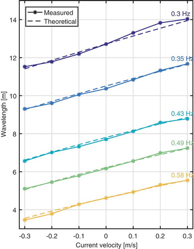
Figure 9. Observed change in wave height for five regular waves in currents ranging from −0.3 m/s to 0.3 m/s. Compared to theoretical wave height change computed from Equation (5).

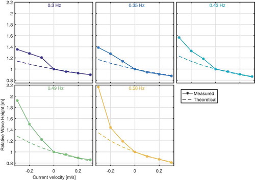
From Figure 9, it is clear that the observed wave heights do not match up with theory. Following current cases appear to agree quite well, yet for the opposing conditions the increase in wave height is much greater than predicted. This has been observed consistently in FloWave, as documented in Draycott et al. (2017), and is thought to be a combination of nonlinear wave–current interaction and tank-specific wave effects. The theoretical wave heights were calculated under the assumption of conservation of wave action, a commonly accepted conserved quantity for wave–current interaction. As the wavelengths appear correctly predicted, it is likely that there is more wave energy being input to the system; i.e. the wave generation is responding to the presence of opposing current. This is possibly due to current-induced head change altering the water level in front of the paddles. As the generation frequencies are unchanged, the wavelengths are still expected to be approximately those predicted from Equation (2), which is what is observed in Figure 8.

Despite the discrepancy between predicted and measured amplitude, the modified dispersion relation appears correct due to the success of wavelength prediction, and as such the inherent assumptions in the presented method are justified.

4.3.2. Incident and reflected wave spectra

The five irregular wave cases defined in Table 1 have been re-created, for each of the seven current velocities. The isolated incident and reflected spectra, calculated using the methodology presented in Section 2, is shown in Figures 10 to 12. Figure 10 displays all of the incident spectra, whilst Figure 11 and Figure 12 show the reflected spectra for the following and opposing current conditions, respectively. From Figure 10, the incident spectra appear to be well isolated, and are particularly well defined for low frequency and/or following current conditions. Isolated spectra appear more noisy in higher velocities with opposing current. This may be, in part, a result of increased nonstationarity introduced by current velocity fluctuations. The resulting temporal variation in component amplitudes and wavenumbers makes the effective isolation of incident and reflected spectra more difficult.

Figure 10. Incident frequency spectra for five PM spectra of differing peak frequency. The data are calculated for spectra created in currents ranging from −0.3 m/s to 0.3 m/s.

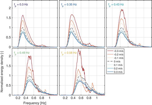
Figure 11. Reflected frequency spectra for waves following current. The data are shown for five PM spectra of differing peak frequency in currents ranging from −0.3 m/s to 0.3 m/s.

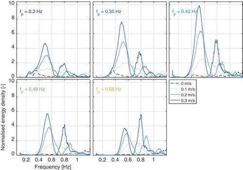
Figure 12. Reflected frequency spectra for waves opposing current. The data are shown for five PM spectra of differing peak frequenc in currents ranging from −0.3 m/s to 0.3 m/s.

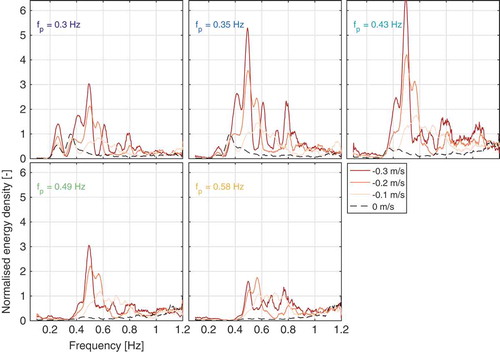
From Figures 11 and 12, it is clear that reflection coefficients increase in larger current, whether opposing or following the waves. It is also apparent that there are peaks in the reflected spectra relating to the phase shift of the waves at the absorption paddles due to the current-induced change in wavelength. This is discussed further in Section 5.3.

5. Discussion

5.1. Effect of incorporating wavelength change in isolating reflections

From the numerical study in Section 3, it is clear that there is a significant improvement in isolation of spectra when the method described in Section 2 is implemented. Without the modification to , incident and reflected spectra will be poorly isolated, the overall magnitudes will be incorrect, and isolated spectra will appear noisy. This has also been observed analogously in all of the experimental results in the FloWave tank. An example of this is shown in Figure 13, where spectrum 2 (=0.35) with 0.3 m/s following current has been re-analyzed without wavenumber correction (essentially the unmodified Zelt and Skjelbreia (1992) method). The same effect is observed in the experimental results as in Figure 4. The overestimation of wavenumber in following current results in an apparent incident spectrum of lesser magnitude with more noise. The corresponding reflected spectrum, while of similar magnitude, exhibits false “harmonic-like” peaks.

Figure 13. Comparison of incident (left) and reflected (right) spectra at FloWave, for a PM spectrum with in 0.3m/s following current. The mean spectrum calculated over the gauges is also shown overlaid.

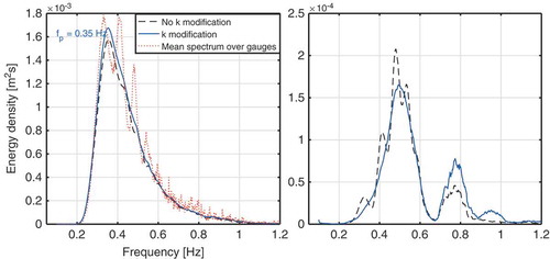
Through both Figure 4 and Figure 13, it is clearly demonstrated that incorporating the wavelength modification improves the calculation of the incident spectrum significantly. This in turn provides a greater level of confidence in the reflected spectrum solution, which exhibits three distinct peaks that differ from the incident spectrum peak. These peaks provide a better understanding of the wavemaker response to changes in wavelengths due to wave–current interaction. From Figures 11 and 12, it is clear that overall reflections increase in the presence of current, whether in opposing or following conditions. Section 5.3 discusses this further.

5.2. Describing and analyzing reflections coefficients in current

The aim of this section is to explore ways of representing reflection characteristics in wave–current conditions as the typical amplitude-based reflection coefficients can be misleading.

Reflection coefficients are typically amplitude based and are calculated using Equation (13). To enable easier assessment, these frequency-dependent reflection coefficients, , can be reduced to a single, amplitude-based overall reflection coefficient for each spectrum via Equation. (14). The results are displayed in Figure 14 for the wave cases defined in Table 1.

(13)

(14)

Figure 14. Observed overall reflection coefficients as a function of current velocity for PM spectra of differing peak frequency.

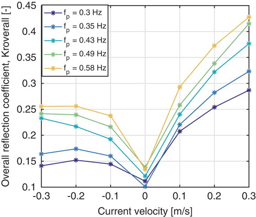
From Figure 14, it appears that the reflections are larger for following current conditions, which is true when only assessing the relative amplitudes in the measurement zone (in current). When trying to assess the actual wave absorption performance in current, these amplitude-based reflection coefficients in the current zone are misleading. Opposing waves are attributed smaller values even if the underlying (current unmodified) reflections are equivalent. This is due to the reflected waves travelling in a following current, resulting in decreased reflected amplitudes. In the same manner, following current cases appear to have increased reflection coefficients due to reflected waves becoming steeper in opposing current. A good example of this is the numerical simulation (Figures 3 and 4) where the underlying (current-unmodified) reflection coefficients were equal for all current velocities, yet the calculated amplitude-based reflections differ greatly. In order to compare the reflection coefficients between different current conditions effectively, it is suggested that amplitude-based reflection coefficients are no longer appropriate.

5.2.1. Wave-action-based reflection coefficients

A quantity termed wave action is often assumed conserved through wave–current interaction (wave energy or wave power are not conserved), and as such using this quantity to define reflection coefficients removes the dependency on current velocity. This allows for effective comparison between different current conditions and allows fairer assessment of absorption performance.

The conservation of wave action is described in Jonsson (1990) by:

(15)

where is the relative angle between the wave and current fields. Noting that , a frequency-dependent wave-action term can be defined as:

(16)

where the subscript defines values relative to the current field and and are defined in Equations (3) and (4). A frequency-dependent wave-action reflection coefficient can therefore be defined as:

(17)

and total wave-action-based reflection coefficients can be described by

(18)

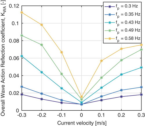
For the numerical example described in Section 3, the wave-action-based reflection coefficients remain unchanged in current (all incident and reflected wave-action spectra are equal). Equation (18) has been used to calculate the total wave-action-based reflection coefficients for the sea states defined in Table 1 and the results are shown in Figure 15. It is evident that the reflections for the opposing and following conditions are now more comparable. Assessing amplitude-based reflection coefficients, it appeared that reflections were worse in following conditions; however, assessing the values, it is clear that actual absorption performance in FloWave is better for following cases. Absorption is worse in opposing conditions due to larger phase differences at the absorbing paddle location (from wavelength modification by current). These values are therefore more representative of the underlying wave reflections and allow effective isolation of wave modification by current and wave reflection from structures or devices.

Figure 15. Observed wave-action-based reflection coefficients as a function of current velocity for PM spectra of differing peak frequency.

5.3. Reflections in wave–current conditions at FloWave

As shown in Figure 3, for a structure with fixed reflection characteristics, one would expect amplitude-based reflection coefficients to increase in following current conditions. This is due to the relative wave height decrease of incident waves, and increase experienced by the reflected waves due to current interaction, irrespective of the structure. The contrary would be expected of opposing waves, where the reflected wavelengths are increased by the current, reducing the reflection coefficient.

Assessing the reflected spectra and coefficients in FloWave (Figures 11, 12, 14, and 15), it is evident that reflections (amplitude or wave-action based) increase with current velocity whether current is opposing or following. Initially, this seems to contradict what is suggested; however, it is worth remembering that the “reflected” waves at FloWave are actually originating from a dynamic system: active force-feedback paddles. Absorption performance and resulting reflection coefficients are therefore highly dependent on the paddles and corresponding control strategy. Without the presence of current, the absorption performance is largely a function of frequency and steepness, with lower frequency–higher steepness conditions having better absorption performance and lower reflections [Draycott et al. (2016)]. This frequency dependency is evident in Figure 15.

When current is included, the wavelengths are altered and so is the desired phase relationship between paddles for optimal absorption performance. There is a predictive element of the control strategy at FloWave which relies on knowledge of the wavelengths and assumes that the standard dispersion relation, Equation. (1), applies. This becomes increasingly inaccurate in larger currents, whether opposing or following, which explains the increased reflection coefficients observed in Figures 14 and 15. It is also suggested that the peaks and troughs observed in the reflected spectra (Figures 11 and 12) are a result of the frequency-dependent phase relationship, at the “absorbing” paddle location, between the current modified and expected waves (unmodified). Troughs occur at close to zero-phase difference (integer number of wavelengths discrepancy) and peaks occur when there is difference.

5.4. Future work and applications

5.4.1. Noncollinear cases (oblique)

The method, application, and results presented have all been for waves with collinear current. In principle, it is fairly simple to extend the approach to allow for waves and currents traveling in any direction. The theoretical Fourier coefficients at wave gauge can be adapted to the 2D problem as follows:

(19)

where and are the angles of the incident and reflected waves of the jth wave component. is now a function of the relative angle between the wave and current fields, :

(20)

where for : and for : . is the current flow direction.

If and are known or well approximated, then this can be solved in the same manner as previously using Equations (8) to (11). The complex values and are the only unknowns and are found by minimizing the difference between theoretical and measured Fourier coefficients, , across all gauges. The problem is that for larger current velocities and higher frequencies (low ) the refraction effects can be non-negligible, and if it is deemed that they cannot be effectively approximated then it is required to solve for and . The numerical scheme implemented does not allow solving for this, and so at present only noncollinear cases when is very small can be appropriately resolved without introducing a model for refraction (which for FloWave is difficult as the flow field is highly complex). Section 5.4.2 discusses the possibility of adapting the numerical solution approach to allow solving for the angles at the measurement location, along with other parameters.

5.4.2. Any deterministic wave field

As mentioned in Section 5.4.1, in some cases, it is desired to solve for additional parameters relating to the incident and reflected spectra. This could be solving for the incident and reflected wave angles or could be solving for values rather than assuming the modified dispersion relation holds. In theory, one could also solve for additional wave systems, e.g., a second reflected system, , from a floating body.

Ideally, it would be possible to define any theoretical Fourier coefficient formulation, designed for the specific problem. From this, all of the wave parameters that are unknown could be resolved by minimizing the weighted sum of square errors across all wave gauges between the measured and theoretical Fourier coefficients, thus resolving any deterministic wave field. This would essentially involve creating a numerical framework that can resolve all of the parameters (or equivalent) in Equation. (19), with the only known values being the gauge positions and measured Fourier coefficients. To avoid ambiguity in resolving the exponential term, a well-designed 2D wave gauge array would be required. A way of resolving complex values and finding a global minimum would need to be found given the constraints of the problem (; etc.). This is fairly challenging and has not been implemented at present; however, it is thought that in future this will be a viable approach to resolving complex deterministic wave systems including multidirectional waves in current.

5.4.3. Dissemination of methodology and code

It is intended that the methodology and code will be made available for use by the scientific community. Once the code has been packaged for external use, the code and associated documentation will be made available. Initially, this will be held on https://www.researchgate.net/profile/Sam_Draycott alongside the publication. In future, a repository will be created on the new FloWave website, http://www.flowave.eng.ed.ac.uk/, alongside other tools developed for wave analysis.

6. Conclusions

The isolation of incident and reflected waves are important to characterize for a wide number of ocean and coastal engineering problems; yet no proven methods exist for when waves are propagating on a current. In this article, a method to isolate incident and reflected wave fields in the presence of colinear current is presented, utilizing a frequency-domain least-squares approach with a modified dispersion relation. The method is shown to be effective in an idealized numerical simulation, before the method assumptions are tested experimentally. It is found that the modified dispersion relation is valid, and assumptions of steady, uniform, and irrotational flow are reasonable approximations. Application of the method to typical wave spectra in current provides insight into wave absorption performance at the FloWave ocean basin, which is aided by the introduction of a wave-action-based reflection coefficient. The presented method will enable reflection analysis to be performed for wave–current conditions more effectively, improving results for both laboratory and open ocean experiments.

Acknowledgements

The authors would like to thank the UK EPSRC for funding the FloWave facility (EP/I02932X/1).

Disclosure statement

No potential conflict of interest was reported by the authors.

Additional information

Funding

This work was supported by the UK EPSRC [EP/I02932X/1];

References

- Chen, H. B., C. P. Tsai, and J. R. Chiu. 2006. “Wave Reflection from Vertical Breakwater with Porous Structure.” Ocean Engineering 33 (13): 1705–1717. doi:10.1016/j.oceaneng.2005.10.014.
- Dickson, W., T. Herbers, and E. Thornton. 1995. “Wave Reflection from Breakwater.” 121 (October): 262–268.
- Draycott, S. 2017. On the Re-creation of Site-Specific Directional Wave Conditions, PhD thesis, Universities of Edinburgh, Strathclye and Exeter.
- Draycott, S., T. Davey, D. M. Ingram, A. Day, and L. Johanning. 2016. “The SPAIR Method: Isolating Incident and Reflected Directional Wave Spectra in Multidirectional Wave Basins.” Coastal Engineering 114: 265–283. doi:10.1016/j.coastaleng.2016.04.012.
- Draycott, S., D. R. Noble, T. Davey, T. Bruce, D. M. Ingram, L. Johanning, and H. C. M. Smith. 2017. “Re-Creation of Site-Specific Multi-Directional Waves with Non-Collinear Current.” Preprint Submitted to Ocean Engineering 1–24. doi.10.1016/j.oceaneng.2017.10.047.
- Frigaard, P., and M. Brorsen. 1995. “A Time-Domain Method for Separating Incident and Reflected Irregular Waves.” Coastal Engineering 24 (3–4): 205–215. doi:10.1016/0378-3839(94)00035-V.
- Goda, Y., and T. Suzuki. 1976. “Estimation of Incident and Reflected Waves in Random Wave Experiments.” Coastal Engineering Proceedings 1 (15): 828–845.
- Hasselmann, K., T. P. Barnett, E. Bouws, H. Carlson, D. E. Cartwright, K. Enke, J. A. Ewing, et al. 1973. “Measurements of Wind-Wave Growth and Swell Decay during the Joint North Sea Wave Project (JONSWAP).” Ergnzungsheft Zur Deutschen Hydrographischen Zeitschrift Reihe A (8): 95. (8 0).
- Highlands and Islands Enterprise 2017. Wave Energy Scotland, May. http://www.hie.co.uk/growth-sectors/energy/wave-energy-scotland/
- Ingram, D., R. Wallace, A. Robinson, and I. Bryden. 2014. “The Design and Commissioning of the First, Circular, Combined Current and Wave Test Basin.” Oceans 2014 - Taipei. https://www.flow3d.com.
- Jonsson, I. G. 1990. “Wave–Current Interactions Chap. 7.” In The Sea, Ocean Engineering Science, eds. B. LeMehaute and D. M. Hanes, 65–120. New York: Wiley-Interscience publications. ISBN 0471633933
- Mansard, E. P., and E. R. Funke 1980. “The Measurement of Incident and Reflected Spectra Using a Least Squares Method.” . 154–172
- Meyer, C., and P. A. Papakonstantinou. 2009. “On the Complexity of Constructing Golomb Rulers.” Discrete Applied Mathematics 157 (4): 738–748. doi:10.1016/j.dam.2008.07.006.
- Moreira, R. M., and D. H. Peregrine. 2012. “Nonlinear Interactions between Deep-Water Waves and Currents.” Journal of Fluid Mechanics 691 (February): 1–25. doi:10.1017/jfm.2011.436.
- Noble, D. R., T. Davey, H. C. M. Smith, P. Kaklis, A. Robinson, and T. Bruce 2015. Characterisation of Spatial Variation in Currents Generated in the FloWave Ocean Energy Research Facility, 11th European Wave and Tidal Energy Conference, Nantes, France. Nantes, France. pp. 1–8.
- Robinson, A., D. Ingram, I. Bryden, and T. Bruce. 2015. “The Generation of 3D Flows in a Combined Current and Wave Tank.” Ocean Engineering 93: 1–10. doi:10.1016/j.oceaneng.2014.10.008.
- Smith, J. M. 1997. One-Dimensional Wave–Current Interaction, Tech. Rep. 9, US Army Engineer Waterways Experiment Station, Coastal Engineering Research Center, ENGINEER RESEARCH AND DEVELOPMENT CENTER VICKSBURG MS COASTAL AND HYDRAULICS LAB.,
- Sutherland, D. R. J., D. R. Noble, J. Steynor, T. A. D. Davey, and T. Bruce. 2017. “Characterisation of Current and Turbulence in the FloWave Ocean Energy Research Facility.” Ocean Engineering 139 (May): 103–115. doi:10.1016/j.oceaneng.2017.02.028.
- Zanuttigh, B., S. M. Formentin, and R. Briganti. 2013. “A Neural Network for the Prediction of Wave Reflection from Coastal and Harbor Structures.” Coastal Engineering 80: 49–67. doi:10.1016/j.coastaleng.2013.05.004.
- Zanuttigh, B., and J. W. Van Der Meer. 2008. “Wave Reflection from Coastal Structures in Design Conditions.” Coastal Engineering 55 (10): 771–779. doi:10.1016/j.coastaleng.2008.02.009.
- Zelt, J. A., and J. E. Skjelbreia. 1992. “Estimating Incident and Reflected Wave Fields Using an Arbitrary Number of Wave Gauges.” Coastal Engineering Proceedings 1: 777–789.