Application of parallel computing in data mining for contaminant source identification in water distribution systems

Abstract

Contaminant source identification (CSI) procedures are drawing increasing attention due to the possibility of accidental and/or deliberate contaminant intrusion into water distribution systems. However, uncertainties that exist in the modeling have the potential to dramatically impact the capabilities of CSI procedures. Nodal demand uncertainties, as they influence false negative and false positive rates of contaminant detection, are examined. A procedure to quantify the false negative rate is provided, and the false positive issue is shown to be related to a parameter ‘m’. Addressing the false positive and negative issues is demonstrated as feasible due to the use of parallel computing in a super-computer, which reduces the elapsed time for 150 scenario simulations from 37.5 hrs to only 15 min in the case study. By increasing the number of scenarios in the database for CSI through the use of a super-computer, the opportunity exists to decrease the false negative rate and reduce the number of false possible intrusion nodes.

Les procédures de l’identification des sources de contamination (CSI) sont en attirant l’attention croissante en raison de la possibilité de contact accidentel et/ou délibéré d’intrusion des contaminants dans les systèmes de distribution d’eau. Donc, les incertitudes qui existent dans la modélisation ont la potentialité de influer considérablement sur les capacités de la procédure de CSI. L’incertitude de la demande indispensables, car elles influencent les faux négatifs et de faux positifs des taux de détection des contaminants, qui sont examinés ici. Une procédure de quantification du taux des faux négatifs est préparée. Ainsi, la question de faux positifs est démontrée être liée à un paramètre ‘m’.

Se référant aux questions de faux positifs et négatifs, il est démontré comme étant dû à l’utilisation possible du calcul parallèle à l’aide d’un supercalculateur. Ce qui réduit le temps écoulé pour 150 simulations de scenarios de 37,5 heures à seulement 15 minutes dans cette étude. Il existe la possibilité pour diminuer ce taux de faux négatifs en augmentant le nombre de scénarios dans la base de donnée pour le CSI avec l’utilisation d’un supercalculateur et de réduire le nombre des faux nœuds d’intrusion possible.

Keywords:

• parallel computing
• contaminant source identification
• uncertainty
• EPANET
• false positive
• false negative

Introduction

The ability to identify the location of a source of contaminant intrusion into a water distribution system (WDS) from deliberate and/or accidental events is drawing increasing attention. Without understanding the intruded contaminant characters, it is impossible to model the transport and fate of the contaminant within a WDS. However, in the case of a real intrusion, it is rarely easy to know the name of the contaminant, even its type (chemical or biological), resulting in real challenges to construct an exact water quality model. Possible solutions include the generation of conservative estimates such as assuming: 1) the contaminant (e.g., chemical) intruded into the network is of sufficient quantity that it will not decay or dilute to null along its path to a node, or 2) the contaminant (e.g., biological) concentration is increasing along its flow path. In either case, the key is to identify the intrusion node as the source node. Placing a sensor network in the WDS is an option for providing security of water supply systems (American Water Works Association (AWWA) 2004). Identification of the presence of a contaminant by the sensor network triggers the contaminant source identification (CSI) procedure. Due to the rapid movement of a contaminant moving along with water within the WDS, the need exists to identify possible sources quickly and accurately, indicating it is unacceptable for a proposed algorithm to require hours or even days. In addition, various uncertainties such as nodal demand uncertainties will impact the ability to identify the intrusion source(s), thus including uncertainty in CSI becomes essential.

Currently, various methodologies exist for CSI algorithms. The first type used, for example, by Shang et al. (2002), employs a methodology to trace back a contaminant particle in discrete time, given a sensor’s first detection time and concentration; however, this procedure cannot determine the contaminant release history (contaminant intrusion time, duration, and mass rate) although it is suitable as a pre-step to reduce the search space for an optimization procedure. A second methodology, a simulation-optimization method based on a reduced gradient method (e.g., Guan et al. 2006) or genetic algorithm (GA), involves considerable runtime due to the necessity to simulate large numbers of injection events using EPANET (Rossman 2000). To accelerate the GA optimization procedure, parallel GA has been proposed (e.g., Sreepathi et al. 2007), which allows simulation of intrusion events with EPANET in parallel; the parallel GA procedure has the following limitations: 1) to utilize this procedure online, a water utility may need to maintain the parallel computing facilities or hardware routinely, since the time of an intrusion event is never known à priori, and hence the computing units may be required at any time. Another option is cloud computing, should the internet access and elapsed time in queue before running parallel GA be guaranteed; 2) there is no guarantee for the GA to converge to the global optimum, i.e., the true intrusion node may not be identified; and, 3) there may be the need for simulating duplicate intrusion events, resulting in need for extensive computational power. Use of a neural network is another alternative (e.g., Kim et al. 2008), which applies sensor response and intrusion events data as the input and output of the neural network; this method has only been tested in a pilot network, and the scale-up to a large network may require considerable offline neural network training time and online computation time from the trained neural network model. Perelman and Ostfeld (2010) proposed a Bayesian network for CSI, which clusters all network nodes, identifying the source cluster based on sensor observations; under nodal demand uncertainty, the clusters may be different and thus lead to different source nodes. Wong et al. (2010) applied manual sampling to gradually reduce the number of possible sources based on the sampling information as more samples are available; however, it is almost impossible to identify the existence of contamination without sufficient background data, which are lacking in manual sampling.

Another procedure is data mining (e.g., Huang and McBean 2009; Shen et al. 2009a, 2009b), which involves ‘mining the database’ with structural query language (SQL). The data mining procedure consists of three steps. Firstly, a database is populated with the array of intrusion events (i.e., the combination of injection nodes, injection times, durations, and mass rates). The assembly of this information is usually very time-consuming due to the large number of possible injection simulation events. However, this overall database is completed offline before a real intrusion event, and hence this effort does not represent a large issue. The second step selects the possible injection nodes (PINs) by querying the pre-populated database table using a SQL sentence, and then quantifies the probability of each PIN as the true source node. The SQL is: “select events that result in first detection time at sensor S between t-m and t+m”, where S is the alarmed sensor, t is the observed first detection time at S, and ‘m’ is an offset value from time t. The ‘m’ value is determined in a statistical way. In the third step, the existence of priority nodes which are upstream of important facilities such as schools, hospitals, and governmental offices is checked. Discussion of the third step is not covered in this paper; details can be found in Shen et al. (2009a, 2009b).

Herein, the application of parallel computing with a super-computer in simulating intrusion events is discussed under various scenarios (demand realizations) with nodal demand uncertainty simultaneously. Based on the scenario simulation results, the statistical characterization of the ‘m’ value is provided for each sensor, thus providing a probability (e.g., 95%) that the true intrusion node is included in the PINs selected. To reduce the false negative rate (the rate of not recognizing the true intrusion node as one of the identified PINs) and the number of false PINs, storing more than one scenario simulation result in database for CSI is proposed as an approach to address uncertainty.

Methodology

Shared Hierarchical Academic Research Computing Network (SHARCNET), a super-computer, provides a means for parallel computing, which consists of over 13,000 cores or processors.

The first step in conducting simulation of injection events using EPANET in SHARCNET is to make EPANET source codes compatible with the Linux operation system. López-Ibáñez et al. (2008) modified EPANET source codes to Linux-compatible, to run EPANET in multi-thread for pump operation optimization. López-Ibáñez et al.’s modification is applied herein. In addition, message passing interface (MPI) is applied to parallelize the running of a designated number of scenarios simultaneously.

For each scenario, the need exists to generate random nodal demands to mimic uncertainty. In EPANET, within a hydraulic time step, nodal demand is quantified by the multiplication of its base demand by a normally distributed pattern factor in the time step. Herein, to generate random demands obeying the normal distribution for each node, within each time step, the mean value is set as the pattern factor from EPANET input file, and the standard deviation is set as 10% of the mean value. It is noted that the probability of getting negative random pattern factors is 7.6E-24, which is a very small probability, and hence, in case a negative number is generated, the number is set to zero. Otherwise, it would be necessary to apply a truncated normal distribution to avoid generating negative nodal demand values. The simulation of the intrusion events within the i^th scenario is completed at the processor i of SHARCNET system. The processor ordinal i is assigned by MPI library. The events and corresponding sensors first detection times and concentrations are stored in the text file i.txt. All generated text files are downloaded from SHARCNET to a local computer, and then are moved to MySQL database tables to analyze the ‘m’ values of each sensor and to be served for CSI.

False positive and false negative rates

Storing a limited number of scenarios in the database for the development of the CSI may cause a true event (real intrusion node, time, duration, and mass rate) to be missed. For example, an event ‘inj’ is detected in the 2^nd scenario; by storing only the 1^st scenario in database, the event ‘inj’ will be missed, leading to a false negative. In CSI, it is also possible that false events are identified along with the true event, referring to false positive, which is related to the ‘m’ value of each sensor.

Before quantifying the false negative rate, it is necessary to determine the number of scenarios required as a benchmark. With increasing numbers of scenarios in a database for CSI, more events are detected. The number of newly detected events per increased new scenario may reduce with increasing total scenarios number. In other words, there may be a point of diminishing return in terms of detecting new events by increasing scenarios number.

To quantify the false negative rate of each specific sensor ‘S’, it is assumed that the total number of events detected by ‘S’ is K, and after the i ^th scenario is stored in database, the number of events detected is k. The false negative rate of sensor ‘S’ is (K-k)/K. It is noted this rate will reduce as more scenarios are stored in the database for CSI.

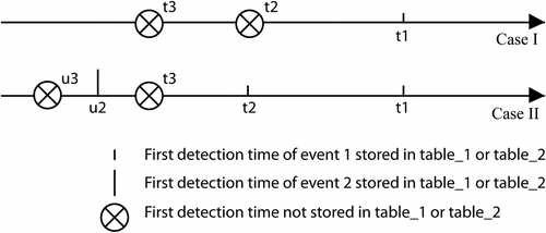
To simplify the illustration process, two intrusion events 1 and 2, denoted as letters ‘t’ and ‘u’ respectively, and three scenarios 1^st, 2^nd, and 3^rd are applied to illustrate the ‘m’ value calculation process. Event 1 is detected in the three scenarios, and event 2 is only detected in the 2^nd and 3^rd scenarios. Two cases I and II are utilized to illustrate the impact of increasing the number of scenarios in the database on ‘m’ value calculation. In Case I, the 1^st scenario is stored; Case II stores both the 1^st and 2^nd scenarios.

Case I

Only detection information of the 1^st scenario is stored, and the resulting database table is named as ‘table_1’. For event 1 in the 1^st scenario, its first detection time at sensor ‘S’ is denoted as t₁ . The statistical analysis for the ‘m’ value is illustrated in Figure 1 “Case I”. For the 3^rd scenario, its offset value from the one in ‘table_1’ t₁ is |t₃ -t₁ |. If applying a SQL against ‘table_1’: “select the injection events that can result in first detection time at S between time t₃ -|t₃ -t₁ | and t₃ +|t₃ -t₁ |”, the true event 1 is selected. Likewise, the offset values of t₁ and t₂ from t₁ are 0, |t₂ - t₁ |. The ‘m’ value is determined as the 95% quantile of the three offset values. To explain the ‘m’ value, 95% of events have offset values below the ‘m’ value; in other words, there is a 95% probability of identifying the true intrusion node in the PINs selected from ‘table_1’, if the true intrusion node is really stored in ‘table_1’.

Figure 1 Offset values analysis in Cases I and II.

Case II

The simulation data of both the 1^st and the 2^nd scenarios are stored in ‘table_2’ (denotes database table containing more than one scenario) for CSI. Figure 1 “Case II” displays the ‘m’ value calculation. u₂ and u₃ are the first detected times of event 2 in the 2^nd and 3^rd scenario at sensor ‘S’. The offset values of event 1 is changed to 0, 0, |t₃ – t₂ | (which is the smaller value of |t₃ – t₁ | and |t₃ – t₂ |); and the offset values of event 2 are 0, |u₃ – u₂ |. The ‘m’ value, after storing the 2^nd scenario, is taken as the 95% quantile of the values of both events 1 and 2: 0, 0, |t₃ – t₂ |, 0, |u₃ – u₂ |. If event 2 is the true event, ‘table_1’ causes a false negative since event 2 is missed. Clearly, by storing one more scenario in ‘table_2’ for CSI, the false negative rate is reduced.

Case study

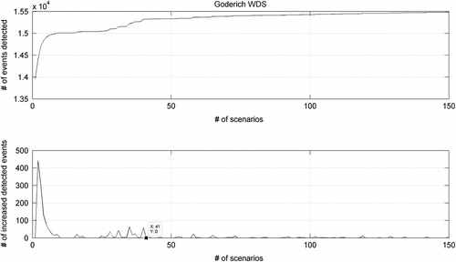
The WDS of the City of Goderich is utilized in the case study. The WDS supplies water for a population of 5,000. The network consists of 285 nodes and 433 links. For water quality simulation, the following parameters are set: duration 72 hrs, hydraulic step 1 hr, and water quality step 5 min. One hundred and fifty scenarios are simulated in parallel with 150 processors of SHARCNET. The total elapsed time is 15 min. Without the parallel facilities of SHARCNET, 15 × 150 min or 37.5 hrs would be required in serial computing. The communication overhead herein is minimal, since each scenario is separate, and no data transfer is needed among the 150 scenarios; thus the extrapolation from single scenario runtime 15 min to 37.5 hrs for the 150 scenarios is reasonable. A finer (smaller) water quality step will capture more accurate sensor response information, which may provide a smaller range of possible intrusion node estimation, with dramatically increased simulation time; where days may be required instead of 37.5 hrs in serial computing. Although the discussion on extending to finer water quality step is beyond the scope of this paper, the parallel computing method described herein provides a way to run the intrusion events simulation in a reasonable elapsed time. The return curve, by increasing the number of scenarios in the database table ‘table_2’ is presented in Figure 2. It is found from the subplot in the second row that after scenario number 41, there are few new events detected (almost all zeros), demonstrating that the number 41 is the point of diminishing marginal return in terms of detecting new events.

Figure 2 Goderich WDS return curve.

Statistical analyses for Case I are listed in Table 1. For sensor node index 81, the false negative rate is 11.7%. If ‘table_1’ is applied for CSI, 11.7% events would be missed, or there would be a 11.7% chance of missing the true event. The corresponding ‘m’ value is 415 min, which means for an online alarm at sensor node 81, there is a 95% chance of identifying the true event from ‘table_1’ if the true one is stored in ‘table_1’.

Table 1. Statistical analysis for cases I and II.

Cases	# of Scenarios in Database	Sensors Index	False Negative Rate (%)	‘m’ Value (min)
I	1	81	11.7	180
		199	13.2	910
		133	21.5	200
		144	22.3	420
		161	10.9	50
II	10	81	3.6	20
		199	2.5	35
		133	7.2	20
		144	5.2	40
		161	3.3	10

In Case II, the 1^st through 10^th scenarios are stored in ‘table_2’. The statistical analysis results are also listed in Table 1. For sensor node index 81, the false negative rate is reduced from 11.7% to 3.6%; the ‘m’ value is changed from 415 min to 20 min.

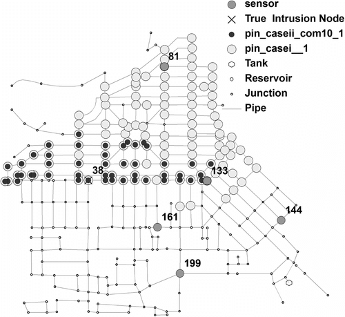
To check the benefit on false positive nodes number reduction gained by applying ‘table_2’ instead of ‘table_1’, a simulated event happening at node index 38 and time 8:00AM is employed. Sensor node index 133 first detected the event at time 9:20 AM. The PINs identification process runtime is less than 1 min, indicating the data mining procedure is sufficiently fast for online CSI application. Figure 3 presents the PINs identified in Cases I and II. Legend ‘pin_casei_1’ shows the PINs in Case I (i.e., storing only the 1^st scenario) after the 1^st sensor alarm, and ‘pin_caseii_com10_1’ represents the PINs identified in Case II (storing the 1^st through 10^th scenarios in ‘table_2’ for CSI) after the 1^st sensor alarm. The number of PINs in Case I is 125, while by utilizing Case II, it is reduced to 49. Both cases identify the true intrusion node index 38, suggesting the accuracy of the proposed CSI procedure.

Figure 3 Goderich WDS-PINs in Cases I and II.

It is shown that the proposed data mining procedure is efficient for real-time CSI, since it can identify the PINs as soon as a sensor alarm in a magnitude of just minutes. Simulating multiple scenarios with a super-computer SHARCNET and storing the results in database for CSI can help to quantify a parameter ‘m’, which in turn is applied in the PINs identification, and sets 95% statistical confidence on the identified PINs including the true event node; and helps to address the false positive/negative issues in CSI, specifically: 1) by reducing the false negative rate, i.e., reducing the chance of missing the true event, and 2) reducing the number of PINs, thereby providing a smaller scope in identifying the location of the true event.

To extend the proposed methodology to large networks with tens of thousands of nodes and links, possibilities may be to increase the water quality step, use a parallel scenario itself instead of the scenario as an entity, or aggregate the network (i.e., simplify it). However, the database construction (i.e., the scenarios simulation) and false positive/negative issues analyses are completed offline, that is, before a sensor alarm is triggered. The time consumed online is querying the database to select the possible intrusion nodes, which is frequently a real concern for CSI; with a well designed index for the database table, the extra time added to the small network applied herein would be minimal.

Conclusions

The parallel computing ability of a super-computer SHARCNET enables the simulation of a number of scenarios under nodal demand uncertainty simultaneously, in a very short time period. The simulation results allow statistical analyses of the ‘m’ value of each sensor, which in turn is applied to identify PINs, and enable the false negative rate (i.e., missing the true event) quantification for each sensor. Without access to parallel computing (i.e., in serial computing), the ability to resolve the false positive/false negative issues would be very time consuming and hence infeasible, especially with finer water quality step and water distribution system with tens of thousands of nodes.

By storing more scenarios in the database table for CSI, the false negative rate of each sensor is reduced; meanwhile, the number of false PINs may be reduced as well.

Acknowledgement

The financial support provided by NSERC Strategic Grant STPGP 336126-06 and the Canada Research Chair program are gratefully acknowledged.

References

- American Water Works Association (AWWA). 2004. Security guidance for water utilities. Accessed October 2009. http://www.awwa.org/science/wise.
- Guan , J. , Aral , M. M. , Maslia , M. L. and Grayman , W. M. 2006 . Identification of contaminant source in water distribution systems using simulation-optimization method: Case study . Journal of Water Resources Planning and Management , 132 ( 4 ) : 252 – 262 .
- Huang , J. and McBean , E. 2009 . Data mining to identify contaminant event locations in water distribution systems . Journal of Water Resources Planning and Management , 135 ( 6 ) : 466 – 474 .
- Kim , M. , Choi , C. Y. and Gerba , C. P. 2008 . Source tracking of microbial intrusion in water systems using artificial neural networks . Water Research , 42 ( 2008 ) : 1308 – 1314 .
- López-Ibáñez , M. , Prasad , T.D. and Paechter , B. 2008 . Parallel optimisation of pump schedules with a thread-safe variant of EPANET toolkit . Water Distribution Systems Analysis , 2008 : 1 – 10 . doi: 10.1061/41024(340)40
- Perelman , L. and Ostfeld , A. 2010 . Bayesian networks for estimating contaminant source and propagation in water distribution system using cluster structure . Water Distribution System Analysis , 2010 : 426 – 435 . doi: 0.1061/41203(425)40
- Rossman , L. A. 2000 . EPANET 2 users manual , Cincinnati , OH : United States Environmental Protection Agency . 200
- Shang , F. , Uber , J. G. and Polycarpou , M. M. 2002 . Particle back tracking algorithm for water distribution system analysis . Journal of Environment Engineering , 128 ( 5 ) : 441 – 450 .
- SHARCNET. Accessed October 2010.https://www.sharcnet.ca/help/index.php/Knowledge_Base
- Shen , H. , McBean , E. and Ghazali , M. 2009a . Multi-stage response to contaminant ingress into water distribution systems and probability quantification . Canadian Journal of Civil Engineering , 36 ( 11 ) : 1764 – 1772 .
- Shen , H. , McBean , E. and Ghazali , M. 2009b . “ Contaminant source identification for priority nodes in water distribution systems ” . In Dynamic modeling of urban water systems, Monograph 18 , Edited by: James , W. 485 – 497 . Guelph : CHI .
- Sreepathi , S. , Mahinthakumar , K. , Zechman , E. , Ranjithan , R. , Brill , D. , Ma , X. and Laszewski , G. V. 2007 . Cyberinfrastructure for contamination source characterization in water distribution system . Proceedings of Computational Science ICCS 2007, Part I, Lecture Notes in Computer Science , 4487 : 1058 – 1065 .
- Wong , A. , Young , J. , Laird , C.D. , Hart , W.E. and McKenna , S.A. 2010 . Optimal determination of grab sample locations and source inversion in large-scale water distribution systems . Water Distribution System Analysis , 2010 : 412 – 425 . doi: 10.1061/41203(425)39