Empirical modelling of maximum weekly average stream temperature in British Columbia, Canada, to support assessment of fish habitat suitability

Abstract

The objective of this study was to characterize the spatial variability of stream thermal regimes in British Columbia, Canada, with the specific goal of developing a predictive model to assist in provincial-scale assessment of fish habitat. It is part of a broader study to develop an approach to support the designation of “Temperature Sensitive Streams”, particularly in relation to the potential effects of forest harvesting and climate change. Stream temperature data were collected from researchers, consultants and government agencies. After checking for data quality, the annual maximum of a seven-day running average of mean daily water temperature (MWAT) was extracted for each station-year. A multiple regression model for the mean MWAT for each station was fitted for stations having basin areas between 1 and 10⁴ km². Predictor variables included the logarithm of catchment area, normal July–August air temperature for the location, the square root of the percentage of glacier cover in the catchment, the square root of the percentage of lake cover in the catchment, the mean catchment elevation, channel slope, a coefficient related to intensity of the mean annual flood, and the deviation of July–August air temperature during the monitoring year(s) from the average during a reference period. Model coefficients were consistent with the physical processes known to govern stream temperature. The standard deviation of prediction errors from a 10-fold cross-validation was 2.1°C. Lack of information on riparian shading is a likely source of a significant portion of the prediction error. The model can be used to provide an initial prediction of stream temperature regime for fish habitat assessment, as well as to provide first-order estimates of the sensitivity of MWAT to climatic warming and glacier retreat.

La présente étude avait pour objectif de caractériser la variabilité spatiale des régimes thermiques des cours d’eau en Colombie-Britannique, au Canada, le but précis étant de concevoir un modèle de prévision afin de faciliter l’évaluation à l’échelle provinciale de l’habitat du poisson. Cette initiative s’inscrit dans une plus vaste étude visant à élaborer une approche pour soutenir la désignation des cours d’eau sensibles à la température, particulièrement en ce qui concerne les effets potentiels de l’exploitation forestière et du changement climatique. Les données sur la température des cours d’eau ont été recueillies auprès de chercheurs, de consultants et d’organismes gouvernementaux. Après vérification de la qualité des données, le maximum annuel d’une moyenne mobile sur sept jours de la température quotidienne moyenne de l’eau (THMM ou température hebdomadaire moyenne maximale) a été extrait pour chaque année-station. Un modèle de régression multiple pour la THMM pour chaque station a été adapté pour les stations ayant une zone de bassin entre 1 et 104 km2. Les variables explicatives comprenaient le logarithme du bassin hydrographique, la température de l’air normale de juillet–août pour le lieu, la racine carrée du pourcentage de la couverture glaciaire dans le bassin, la racine carrée du pourcentage de la couverture lacustre dans le bassin, l’altitude moyenne du bassin hydrographique, la pente du canal, un coefficient lié à l’intensité de la crue annuelle moyenne et l’écart de la température de l’air en juillet–août au cours de l’année ou des années de surveillance par rapport à la moyenne pendant une période de référence. Les coefficients du modèle étaient conformes aux processus physiques reconnus comme étant des facteurs qui régissent la température des cours d’eau. L’écart-type des erreurs de prévision d’une validation croisée multipliée par dix était de 2,1 C. Le manque de données sur l’ombrage riverain est probablement à l’origine d’une bonne partie de l’erreur de prévision. Le modèle peut servir à offrir une prédiction initiale du régime thermique du cours d’eau pour l’évaluation de l’habitat du poisson, ainsi qu’à fournir des estimations de premier ordre de la sensibilité de la THMM au réchauffement climatique et au recul glaciaire.

Keywords:

• stream temperature
• multiple regression
• fish habitat
• maximum weekly average temperature
• MWAT
• British Columbia
• Temperature Sensitive Stream

Introduction

Stream temperature has been called the master variable in aquatic ecosystems. It controls rates of biological and chemical processes, can limit dissolved oxygen concentrations, and plays an important role in controlling the life history and behavioural ecology of aquatic organisms, including invertebrates, amphibians and both resident and anadromous fish species (e.g., Vannote and Sweeney 1980; Holtby 1988; Richter and Kolmes 2005; Welsh and Hodgson 2008). Therefore, characterizing a stream’s thermal regime is critical to assessing its habitat suitability for fish and other aquatic species. Changes in stream temperature resulting from land use and climate change can potentially have negative influences on aquatic ecosystems, particularly for cold- and cool-water species such as salmonids, and there has been increasing attention in British Columbia and elsewhere to identifying “Temperature Sensitive Streams” (TSS) (Reese-Hansen et al. 2012). These are streams for which temperature increases associated with forest harvesting or other human activity may push the stream above a threshold for a particular species, such as bull trout (Salvelinus confluentus), or have negative effects on one or more aspects of a species’ life history (Nelitz et al. 2007).

The Government of British Columbia, in its Forest and Range Practices Act (2004), provides for the designation of “Temperature Sensitive Streams” (TSS) to protect fish habitat. Following such a designation, further forest harvesting along the designated stream reach or its immediate tributaries could be subject to restrictions, particularly within or near the stream’s riparian zone. Given the potential economic costs to forest companies following TSS designation, the procedure used to support designation must be based on sound science and models that have been tested using the best available data sets. A research project was initiated in 2004 to develop and provide a proof-of-concept for a framework to designate TSS. The framework adopts an ecological rather than biological approach by providing an assessment of the risk that forest harvesting activity, either on its own or in combination with climate warming, could increase stream temperatures sufficiently to cause a shift in the fish species assemblage in the affected reach.

The framework incorporates two empirical models: one for predicting “baseline” stream temperature regimes from existing spatial databases, using variables describing catchment characteristics and reach-scale climate; and one to relate fish species assemblages to an index of stream thermal regime. The specific objective of the current paper was to develop a model for predicting current stream temperature regimes over British Columbia, Canada, which covers approximately 95 million hectares and is highly diverse in its range of climate, topography, hydrologic regime and vegetation (Eaton and Moore 2010; Moore et al. 2010). In particular, an empirical model was developed to predict the Maximum Weekly Average Temperature (MWAT), a metric computed as the annual maximum value of a seven-day running average of daily mean water temperatures. The remainder of this article first outlines the rationale for choosing MWAT as the key temperature metric and the reasons for choosing an empirical approach rather than a deterministic modelling approach, followed by a description of data compilation and analysis. Potential applications of the model are outlined for assessing thermal suitability for fish and its sensitivity to climatic warming and glacier retreat.

Background

Temperature metrics

A variety of stream temperature metrics are in use for regulatory, assessment and management purposes, including the annual maximum (T _max), seasonal mean (T _mean) and seasonal median (T _med), the annual maximum of a seven-day running average of mean daily temperature (MWAT) and the annual maximum of a seven-day running average of maximum daily temperature (MWMT). In addition, metrics such as the rate of warming and daily temperature range can be appropriate in some contexts (e.g., Chu et al. 2010). For this study, we chose MWAT as the key index of thermal regime. Sullivan et al. (2000) and Nelitz et al. (2007) found that MWAT correlated well with various aspects of the life history of salmonids (as inferred from bioenergetic modelling), while many studies have related fish species distributions and thermal tolerances to MWAT or related indices (e.g., Eaton et al. 1995; Eaton and Scheller 1996; Welsh et al. 2001; Wehrly et al. 2003, 2007; Ruesch et al. 2012). Furthermore, MWAT is correlated with both summer maximum and mean temperatures (Table 1) and therefore should be a reasonable compromise metric to characterize these aspects of summer stream temperature regimes.

Table 1. Strength of relations between temperature indices, expressed as r ², including annual maximum (T _max, expressed as the maximum hourly temperature in a given year), maximum 7-day mean (MWAT), maximum 7-day mean of daily maximum (MWMT), seasonal mean (T _mean) and seasonal median (T _med).

		Study
Metrics	Sullivan et al. (2000)	Lewis et al. (2000)	Scholz (2001)	Nelitz et al. (2007)
T max and MWMT	> 0.99	> 0.99	0.98	0.98
T max and MWAT	0.87	0.92	0.57	0.88
MWAT and MWMT	0.89	0.93	0.63	0.92
T max and T med	0.59	n/s^1	n/s	0.92
MWMT and T med	0.62	n/s	n/s	0.94
MWAT and T med	0.83	n/s	n/s	0.98
MWAT and T mean	n/s	n/s	> 0.99	0.98
n	19	n/s	39	104
Study location	Coast Range and Western Cascades, Washington	Northern California	Eastern Cascades, Washington	Central British Columbia
^1 n/s = “not specified”

Modelling approaches

Stream temperature models lie on a spectrum between those based on empirical relations and those based on physical principles including energy and water balances. While catchment-scale physically based models could, in principle, serve as tools for predicting stream temperature variations both within and among catchments, their practical utility is limited at present by the great amount of input data required to run them, although advances in geographic information systems (GIS) technology and the increasing availability of land cover and topographic data may alleviate this challenge to some extent. However, distributed models also require significant time and effort to develop a model application for a specific catchment. For example, Chen (1996, cited in Chen et al. 1998a) based his doctoral research project around the application of the Hydrologic Simulation Model – Fortran (HSPF) model to predict stream temperatures within a single basin, the Upper Grande Ronde catchment in northeast Oregon (1780 km²).

Despite the investment in data and effort needed to develop applications of distributed models, such models do not necessarily provide a high level of predictive accuracy. For example, Sullivan et al. (1990) found that three catchment-scale models (QUAL2E, SNTEMP and MODEL-Y) did not provide accurate temperature predictions for forested catchments in Washington. In Chen’s study, the root-mean-square error (RMSE) for predictions of MWMT was 2.8°C, with differences between predicted and observed temperatures at individual locations ranging from –2.2°C to 7.7°C (Chen et al. 1998b). Allen et al. (2007) developed a simplified mechanistic model that predicts a metric essentially equivalent to MWAT. When applied to several basins in northern California, it generated predictions with RMSE less than 0.4°C. However, the model requires measurements of stream discharge at various locations through the basin to allow accurate specification of groundwater discharge rates, and also requires tuning of some of the model parameters. Given the sparse hydrometric network in British Columbia, a model such as Allen’s would be difficult to apply across the entire province.

A number of studies have developed statistical models for predicting regional stream temperature variability (Wehrly et al. 1998, 2009; Lewis et al. 2000; Isaak and Hubert 2001; Scholz 2001; Scott et al. 2002; Nelitz et al. 2007; Tague et al. 2007; Daigle et al. 2010; Hrachowitz et al. 2010; Isaak et al. 2010; Kelleher et al. 2011; Mayer 2012; Ruesch et al. 2012). Predictor variables in the models included one or more static indices representing catchment scale, macroclimatic context, catchment-scale land use (e.g., cattle density and deforestation) or land cover (e.g., % lake coverage, % glacier coverage), reach-scale characteristics such as shading by riparian vegetation and gradient, and hydrogeologic indices (e.g., soil permeability and baseflow index). At a finer scale, one model included a dummy variable to distinguish pool sites from riffles (Lewis et al. 2000). Catchment scale has normally been expressed as drainage area, stream order or stream distance from the drainage divide. Macroclimate of the monitoring location has been represented using either climate variables, including air temperature and precipitation, or geographic variables such as latitude, longitude, elevation and distance from the crest of a mountain range. Reach-scale shading has been characterized using variables such as field-measured canopy closure or canopy cover, variables representing the presence or extent of riparian trees or forest cover, or potential direct solar radiation modified to account for riparian shading. In addition to these static indices, some models have incorporated measures of hydroclimatic conditions at the time of monitoring, such as air temperature and streamflow.

Some studies that developed statistical models have addressed the fact that stream temperature exhibits spatial autocorrelation that is structured by the stream network (Gardner et al. 2003; Peterson and Ver Hoef 2010). For example, two stations located upstream/downstream of each other along a channel should be more highly correlated than two stations that may be on the same network (i.e., they share a common outlet point somewhere downstream), but do not have any shared drainage area. Isaak et al. (2010) found that spatial models with covariates provided substantially better performance during calibration than non-spatial regression models; the root-mean-square of prediction errors (RMSPE) was 1.45°C for the spatial model and 2.76°C for the non-spatial model (n = 728). However, the difference in performance was smaller for an independent test set, with RMSPE = 2.51°C for the spatial model and 2.78°C for the non-spatial model (n = 52). Ruesch et al. (2012) found that the two covariates in their geostatistical model, representing exposure to solar radiation and air temperature, explained 71% of the variance in MWAT, while the spatial autocovariance component of the model explained 13%. However, both those studies involved relatively dense monitoring networks: over 100 stations per 1000 km² for the study by Isaak et al. (2010) and 14 stations per 1000 km² for the study by Ruesch et al. (2012). In their development of statistical models to predict July mean stream temperature in Michigan and Wisconsin, Wehrly et al. (2009) considered that their data were too sparse to apply a network-based geostatistical model, with 820 stations in Michigan and 310 in Wisconsin. Wehrly et al. (2009) compared the performance of a suite of methods, including multiple regression, kriging using Euclidean distance to estimate the error covariance structure, Generalized Additive Modelling and two variations on mixed-effects modelling. They concluded that linear mixed-effects models with a smoothing spline yielded the best performance, but that the difference among methods was slight.

An important source of variability in regional stream temperature is the effect of interannual variability in hydroclimatic conditions, particularly in studies where stream temperature data were compiled from a range of sources over more than one season. Some studies used data from a single season, thereby avoiding issues of interannual variability (e.g., Sullivan et al. 1990; Scholz 2001). Wehrly et al. (1998) collected data for several years, but arbitrarily chose data for a single year for each stream. For each monitoring site, they used air temperature data for the same year as a predictor variable, an approach that should help account for interannual variability. Nelitz et al. (2007) similarly used data for only one year for each station, with summer air temperature for that year at the closest weather station used as a candidate predictor variable. Nelitz expressed air temperature as the deviation for a given year from the average for a reference period. As an alternative approach, Wehrly et al. (2009) averaged the stream temperatures for each station having more than one year of data.

Data sources, processing and analysis

Stream temperature data

Stream temperature data were obtained from consultants, researchers and government agencies. Data covered a range of years from the 1980s to 2005. Unfortunately, not all data were usable. Some data were excluded due to uncertainties regarding monitoring locations. In some cases, the coordinates provided did not fall on any mapped stream and could have conceivably been located on one of two or more nearby, unnamed tributaries. In other cases, the station locations were described with reference to bridges along roads that did not appear on any of the available maps. Lewis et al. (2000) reported similar problems as being among the most significant barriers to the use of donated data for development of empirical models.

Data were received in a variety of formats. Most files contained raw stream temperature data sampled at intervals from 10 minutes to 24 hours. Some files contained daily minimum, mean, and maximum temperatures, and others contained both raw data and daily summary values. In cases where both raw and daily data were available, the raw data were used. All processing and formatting of data files were performed with copies of the original data in order to avoid human-induced corruption. Additionally, this allowed data checking protocols to utilize the original data files for visual comparison with formatted files.

Visual error checking was based on procedures described in Appendix A of Lewis et al. (2000). Plots were examined for errors caused by file conversion (FC), sensor de-watering (SDW), ambient air temperatures prior to sensor placement or following removal (AMB), unit malfunction (UMF) and dead or dying batteries (DB). No stream temperature values were changed. Instead, data that were deemed to be in error were removed from the data set. A discrepancy log was kept in which the type and description of errors, as well as the dates of removed data, were recorded. In cases where FC, AMB, and SDW errors were obvious, they were removed without contacting data donors. In cases of uncertainty, the donor was contacted before suspect data were removed.

Catchment characteristics

Several of the stations had global positioning system (GPS) or map-derived coordinates of their location, but many did not. For stations with no coordinates, the provincial gazetteer was used to obtain the coordinates of the stream on which the station is located, aided by narrative information on the site location (e.g., “station located on left bank approximately 100 m upstream of highway bridge”). All station coordinates were converted to the Albers projection, which is the British Columbia government standard for provincial-scale mapping applications. Drainage area boundaries for each monitoring site were determined from a digital elevation model (DEM), and a range of catchment characteristics were extracted from the DEM and provincial-scale GIS databases, including basin area (A), fractional glacier area (f _g) and lake area (f _l) within the catchment, mean elevation within the catchment (z _m), slope of the channel segment (derived from 1:50,000 digital maps) containing the monitoring location (slope), and total length of the channel network located upstream of lakes, as a fraction of the total length of channels (f _llen). All GIS and DEM analyses were conducted using ArcGIS. The candidate predictor variables were chosen based on physical process considerations and also the results of an earlier analysis of provincial-scale stream temperature variability based on routine spot temperatures recorded by Water Survey of Canada technicians (Moore 2006).

While riparian shading is an important control on stream temperature (e.g., Moore et al. 2005a), there are no data sources at the provincial scale that would allow it to be quantified with appropriate accuracy. This problem is particularly acute in catchments subject to logging and resource road construction, for which riparian shading will not be constant, and any available riparian data may not be representative of the period covered by stream temperature data. Neglecting the effect of riparian shading is acknowledged as a potentially important source of error.

The k ₂ parameter developed by Eaton et al. (2002) was extracted for each station from a digital map for use in estimating the two-year flood and channel bankfull width. Eaton et al. (2002) generated the digital map by scaling the two-year peak flow at hydrometric stations to an equivalent flow for a 1 km² catchment, using an assumed 0.75-power-law relation between peak flow and catchment area; these values were then interpolated over British Columbia using Kriging. The two-year flood (Q ₂) (m³ s^–1) was calculated as follows:

(1)

Bankfull width (W _b) (m) was included as a candidate predictor variable because it is an important control on riparian shading (wider streams are less well shaded). It was estimated based on the assumption that it scales with the square root of the two-year flood, which has been found to apply for a range of erodible channels (e.g., Simons and Albertson 1963; Hey and Thorne 1986):

(2)

M. Church [University of British Columbia (UBC) Department of Geography, pers. comm.] reports that this relation with c 3.17 is reasonable for cobble bed rivers in BC (based on reported results in UBC theses). In this study, W _b computed from Eq. (2) with c = 3.17 was included as a candidate predictor. However, the choice of values for c is not critical because it would be overridden by the fitted regression slope in the regression model. The k ₂ factor was also included as a candidate predictor variable because its spatial distribution is highly correlated with annual precipitation.

Climate information

Two types of climate information were used in the statistical modelling. To characterise the spatial variation in site macroclimate, monthly normals of air temperature and precipitation, representing averages for 1971–2000, were generated using the ClimateBC application (Hamann and Wang 2005; Spittlehouse 2006), now known as ClimateWNA (Wang et al. 2012). Given that MWAT dominantly occurs from mid-July to late August (see results), the average of the July and August normals for mean air temperature was used as an index of the summer thermal climate. The monthly precipitation normals were summed to yield an annual precipitation normal, which is intended to represent the contrast between maritime and continental locations.

To characterize the interannual variability in climate at each location, a time series of daily air temperature was generated for each station for the period 1990 to 2003 by interpolation of data from surrounding climate stations using the application developed by Stahl et al. (2006), using the constrained lapse rate option. For each year, the interpolated daily air temperatures for July and August were averaged for each station. These July–August means were then expressed as a deviation from the average July–August temperature over the reference period:

(3)

where T _a(i,t) is the July–August air temperature for station “i” and year “t,” T _ref(i) is the mean July–August air temperature for the reference period (1990–2003), and T _a(i,t) is the deviation for station “i” and year “t”.

Statistical analysis

Because the focus was on nominally third-order streams, with typical drainage areas from 10 to 10³ km², the analysis only included those stations with drainage areas between 1 and 10⁴ km². Initial analyses examined the timing of MWAT as well as the variability of MWAT among stations and also among years at individual stations. All analyses were conducted using the software package R (R Core Development Team 2013).

Multiple linear regression was used to fit the predictive model. Given the sparse distribution of stations, we did not attempt to apply a network-based geostatistical model, given the non-trivial computational effort required to process the stream network information. The first stage of model fitting included all of the candidate predictor variables and exclusion of those that were not statistically significant. Where more than one variable represented the same effect (e.g., f _l and f _llen), alternative models were examined and the preferred variable selected based on the degree of fit. Degree of fit was judged partially in terms of the residual sum of squared errors. In addition, plots of residuals against fitted values and against the individual predictors were generated to assess whether the assumptions of linear regression were valid and, in particular, to identify any nonlinear relations. For example, Moore (2006) found that monthly median temperatures typically had a concave-down relation with the logarithm of drainage area. Interactions among variables were also considered during model fitting.

For many stations, data were available for more than one year. The problem with including all station-years in the analysis is that the observations are not independent, contrary to a key assumption underlying regression analysis. The use of mixed-effects linear models can, in principle, deal with this type of repeated measures data structure. However, the implementation in R (lme4) was unable to handle the number of levels of “station” in this data set. Therefore, similar to the approach of Wehrly et al. (2009), we computed the average MWAT value for each station, along with the mean of the air temperature deviations (Eq. 3) for the years with MWAT values. This approach yields one MWAT value and one air temperature deviation per station, thus maintaining independence while still including the information available for stations with multiple years of data.

Following identification of the best model, its predictive accuracy was assessed using cross-validation (Neter et al. 1996). The data were randomly split into 10 roughly equal groups. For each group, MWAT was predicted using a regression based on the other nine groups. Prediction errors (predicted – observed MWAT) for the 10 groups were then combined and examined to assess model performance. While this approach is not as rigorous as using an entirely independent data set for model testing, it is better than simply using the residuals from the regression fit to the entire data set to determine predictive accuracy.

Results

Overview of station characteristics

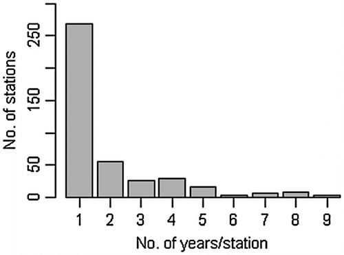
After quality checking and selecting stations by catchment size, data were available for 418 stations (Figure 1). The number of years of data at each station ranged up to nine, with an average of just under two (Figure 2). Only 22 stations had six or more years of data, while 64% of the stations only had one year of data.

Figure 1 Locations of stream temperature monitoring sites within British Columbia, Canada.

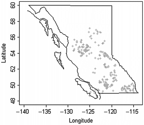
Figure 2 Distribution of numbers of years of data per station.

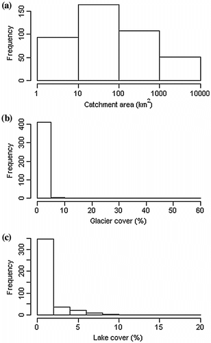
There was a reasonably even distribution of drainage areas within the sample (Figure 3a). Glacier cover ranged up to 51%, although over 98% of stations had less than 5% glacier cover (Figure 3b). Lake cover (Figure 3c) and the fraction of stream length upstream of lakes (not shown) had similar distributions and were reasonably well correlated, with Pearson’s r = 0.80.

Figure 3 Histograms of key characteristics for catchments included in the analysis.

Variability in MWAT and its date of occurrence

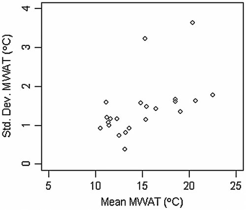
MWAT occurred in July or August in almost all station-years, with most occurrences from mid-July to the end of August (Figure 4). The mean MWAT at each station ranged from less than 5°C to over 20°C, with a mode in the interval from 10 to 15°C (Figure 5). For stations with six or more values of MWAT, the standard deviation generally ranged from 1 to 2°C, with two stations having standard deviations in excess of 3°C (Figure 6).

Figure 4 Histogram of date of occurrence of Maximum Weekly Average Temperature (MWAT) for all station-years included in the analysis. The date shown is the first day of the 7-day period in which MWAT occurred.

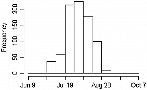
Figure 5 Histogram of mean Maximum Weekly Average Temperature (MWAT) for stations included in the analysis.

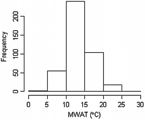
Figure 6 Standard deviation versus mean Maximum Weekly Average Temperature (MWAT) for all stations with six or more years of data.

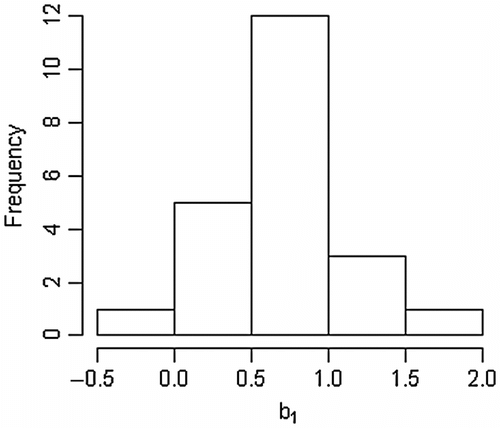
For the 22 stations with six or more years of data, MWAT generally had a positive relation with July–August air temperature, although the strength of the relation varied substantially among stations (Figure 7). The sensitivity of MWAT to summer air temperature, as expressed by the slope of the regression, varied from slightly negative to near 2, with an average of 0.72 (Figure 8).

Figure 7 Lattice plot of relations between Maximum Weekly Average Temperature (MWAT) and July–August air temperature for stations with six or more years of data. Least-squares regression lines are added to each panel. The numbers in the shaded cells indicate station number.

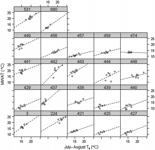
Figure 8 Histogram of the slopes of regressions between Maximum Weekly Average Temperature (MWAT) and July–August air temperature at stations with six or more years of data.

Statistical modelling of MWAT

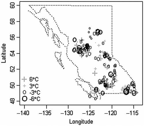
The best model is summarised in Table 2. The cross-validation yielded relatively even scatter for the range of predicted values (Figure 9). The prediction errors are approximately normally distributed (Figure 10) and have a standard deviation of 2.1°C. Scatterplots of prediction errors against the predictor variables do not indicate any obvious problems with lack of fit (Figure 11). Positive and negative prediction errors are spatially interspersed through most of British Columbia, suggesting a lack of regional bias, except in the northeast, where negative errors dominate (Figure 12). A semi-variogram of the cross-validation errors based on Euclidean distance between the stations (not shown) indicated a pure nugget model (or nugget to sill ratio of 1), i.e., no spatial autocorrelation.

Table 2. Coefficients in the best regression model.

Term	Estimate	Std. Error	t value	Pr(>|t|)
Intercept	7.91	1.10	7.19	3.11e-12
T a	0.484	0.07334	6.60	1.32e-10
log(A)	1.18	0.168	6.99	1.16e-11
z m	–0.00306	0.000404	–7.59	2.57e-13
slope	0.0529	0.0214	–2.47	0.014
f g ^0.5	-9.43	1.81	–5.201	3.14e-07
f l ^0.5	17.5	1.67	10.7	< 2e-16
k 2	–0.719	0.182	–3.967	8.79e-05
T	0.644	0.130	4.97	1.00e-06
Ta = normal July-August air temperature (°C); A = catchment area (km^2); zm = mean catchment elevation (m); slope = channel slope (m/m); fg = fractional glacier coverage; fl = fractional lake coverage; k2 = k factor; dTa = difference in July-August air temperature in the monitoring period from that in a reference period (°C)

Figure 9 Observed vs. predicted Maximum Weekly Average Temperature (MWAT) based on the cross-validation. The solid line shows perfect agreement. The dashed line is a quadratic fit to one-sided 90% prediction limits computed for each point during cross-validation.

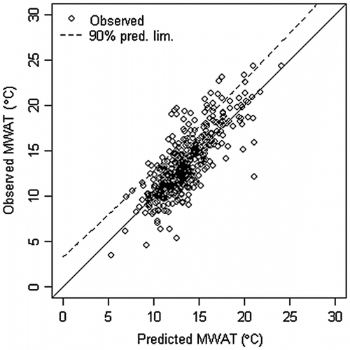
Figure 10 Histogram of prediction errors (predicted – observed) from the cross-validation.

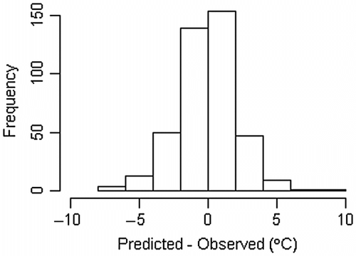
Figure 11 Scatterplots of prediction errors (predicted – observed) from the cross-validation against the predictor variables.

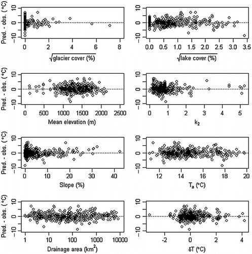
Figure 12 Spatial pattern of prediction errors (predicted – observed) from cross-validation.

Discussion

Evaluation of the regression model

A common challenge in landscape-level statistical modelling is that many catchment-scale variables are correlated (e.g., catchment area and channel slope), leading to an inflation of the standard errors associated with the estimated coefficients. The process for selecting predictor variables included manual intervention to allow for examination of residual plots and to avoid including redundant predictors. Variance inflation factors computed for the final predictor variables were all less than 2.5, suggesting that multi-collinearity is not a severe problem (Neter et al. 1996).

The regression model is consistent with our understanding of the physics governing stream temperature regimes. For example, the increase of approximately 1°C with each order of magnitude increase in catchment area is consistent with previous empirical evidence and process considerations (Caissie 2006). The positive relations between MWAT and air temperature, both temporally and spatially, are consistent with a large volume of past research on the relation between stream and air temperature (e.g., Webb and Nobilis 1997; Mohseni and Stefan 1999; Moore 2006). While the relation between stream and air temperature has been demonstrated to be nonlinear and has been modelled using a logistic curve (Mohseni et al. 1998; Webb et al. 2003; Morrill et al. 2005), the stream temperatures encountered in British Columbia primarily fall in the range for which the relation is roughly linear. Furthermore, including a quadratic term for air temperature, to account for possible nonlinearity in the relation, actually decreased the adjusted R ².

The decrease in MWAT with glacier cover is consistent with the fact that glacier melt augments streamflow during hot, dry weather (Stahl and Moore 2006), thus providing a thermal buffering effect relative to non-glacier-fed streams (Brown et al. 2006; Moore 2006). The linear relation between MWAT and the square root of glacier cover indicates that the sensitivity of MWAT to glacier cover decreases as glacier cover increases. This finding is consistent with the nonlinear sensitivity of stream temperature to discharge; that is, stream temperature becomes increasingly sensitive to changes in discharge as flow decreases (Gu et al. 1998; Moore et al. 2005b).

The increase in MWAT with lake cover is consistent with field observations by Mellina et al. (2002) and arises in part because, during the hot weather that usually generates the MWAT each year, the epilimnion layer of lakes can become substantially warmer than the equilibrium temperature for most streams. The elevated temperatures can persist for some distance downstream. In a proglacial context, Richards et al. (2012) demonstrated that warming between the inlet and outlet of a proglacial lake (a distance of about 300 m) equalled or exceeded the warming that occurred in a 1-km-long segment of stream between the proglacial lake and treeline.

The decrease in MWAT with mean catchment elevation likely results from the advection of cooler source waters from the headwaters, relative to catchments with lower mean elevations. The negative relation between channel slope and MWAT likely reflects the fact that steeper streams tend to have more confined valleys and thus experience greater topographic shading. It could also relate to greater advection of cool water from higher-elevation headwaters. Bankfull width was not significant, possibly because the regional models used to estimate it did not provide reliable predictions. However, the k ₂ factor used in calculating the two-year flood and bankfull width was a significant predictor. The k ₂ factor is a measure of streamflow intensity during flood events, and appeared to be a better index of hydroclimatic conditions than annual precipitation.

The standard deviation of the errors from cross-validation, 2.1°C, is similar to the root-mean-square errors reported for regional models applied in Michigan and Wisconsin, which were 2.0 and 2.3°C, respectively (Wehrly et al. 2009). Wehrly et al. (2009) concluded that much of this prediction error is associated with local-scale phenomena that cannot be adequately resolved with currently available data sets and would require more detailed field data collection. This is likely the case in our study. For example, the lack of reliable measures of riparian canopy shading is a probable source of much of the scatter about the regression, particularly for the smaller catchments, where riparian vegetation can have a major influence on stream temperature. Another potential source of uncertainty is reach-scale thermal heterogeneity associated, for example, with local discharge of groundwater or hyporheic water. Reach-scale variability of up to a few degrees has been documented in a number of studies focused on a range of stream sizes (e.g., Bilby 1984; Clark et al. 1999; Ebersole et al. 2003; Moore et al. 2005b). Another possible cause of prediction error is flow withdrawals. Particularly in the warm, arid interior valleys, water is withdrawn from many streams for irrigation. Since water temperature tends to increase with decreasing flow (Hockey et al. 1982; Gu et al. 1998), such withdrawals would likely lead to elevated water temperatures, particularly in hot, dry weather. Unfortunately, there is inadequate information available on withdrawals, particularly in past years, to allow us to include this effect in the model. Finally, there is uncertainty in the predictor variables estimated from spatial databases.

Model applications

The primary motivation for developing the model was to predict current stream temperature regimes to assess thermal habitat suitability and to support TSS designation when applied in combination with a model relating fish community species composition to MWAT (Nelitz et al. 2008). However, landscape-scale models of stream temperature have a range of other applications. For example, streams that plot substantially above the regression prediction could be considered to be abnormally warm given their geographic context, possibly reflecting thermal impairment due to human activity. The Nicola River, for example, has little riparian shading and regulated flow, and has experienced temperature-related salmon mortality. For that river, the observed MWAT (22.5°C) is more than a standard deviation greater than the predicted MWAT (19.9°C). It would be useful to scrutinize more of the outliers to ascertain whether they occur under similar circumstances. If so, then the model could have value as a screening tool to identify streams that could potentially benefit from restoration activities. It should be noted, however, that many streams used to fit the model lie in catchments that have experienced a range of impacts associated with human activity (e.g., forest harvesting, flow withdrawals); the baseline represented by the model does not, therefore, represent “pristine” conditions.

In addition to assessing current thermal habitat, the model could also be used to generate first-order estimates of the sensitivity of MWAT to changes in summer air temperature and glacier cover. For example, the model suggests that a 1°C increase in July–August air temperature would be associated with about a 0.7°C increase in MWAT. An increase in summer air temperature of 2.5°C lies close to the middle of the range of future climate scenarios for BC in 2050 (Moore et al. 2010). If the sensitivity derived from the regression model is applicable to future climate conditions, summertime warming of 2.5°C would be associated with an increase in MWAT of about 1.7°C. Note that this application implicitly assumes that the correlation between summer air temperature and other conditions, such as streamflow, remains consistent into the future.

The coupled effects of climatic warming and glacier retreat could also be estimated. For example, suppose a catchment currently has 10% glacier cover, which would decline to 5% by 2050 in association with a 2.5°C warming. The regression model suggests that the loss of glacier cover could contribute an additional 0.9°C increase in MWAT, for a total increase of 2.6°C. For a catchment that currently has 5% glacier cover, which melts completely by 2050, the additional warming would be 2.1°C, for a total warming of 3.8°C. It would be useful to verify these space-for-time inferences of the sensitivity of stream temperature to changing glacier cover with more detailed process-based modelling in specific catchments.

Directions for future work

Despite the modest predictive ability of the regression model, it has still proven capable of characterizing thermal suitability for fish communities using a risk-based framework (Nelitz et al. 2008). The next step in model development should focus on region-specific models using data collected specifically for the purpose. In this way, data can be collected and processed according to uniform standards, with full certainty regarding station location and assessment of reach-scale temperature variability. In addition, consistent information on riparian conditions, flow withdrawals and other effects of human activity can be documented and incorporated into the model for predicting baseline stream temperatures. Further, at the regional scale it is more feasible to apply models that explicitly address spatial autocovariance associated with the stream network structure. In parallel with work focused on improving empirical modelling of stream temperature, research should focus on developing physically based models that can be parameterized and run using data sources that are currently available, or could reasonably be assumed to be available in the near future.

Conclusions

The Maximum Weekly Average Temperature (MWAT) is correlated with a range of other metrics of summer stream temperature, and usually occurs between mid-July and late August. At a given location, MWAT can vary substantially from year to year, in large part in response to variations in July–August air temperature, with a mean sensitivity of about 0.7°C increase in MWAT per 1°C increase in air temperature. A regression model was generated for predicting the maximum weekly average stream temperature for streams in British Columbia, Canada, based on catchment and climatic characteristics. The model coefficients are consistent with our understanding of the physical processes governing stream temperature. Cross-validation suggests that prediction errors have a standard deviation of about 2.1°C, and the errors display no obvious systematic spatial patterns. A likely source of predictive uncertainty is the lack of information available to characterize riparian shading and water withdrawals. The model can be used to characterize current stream thermal regime and fish habitat suitability, as well as to generate first-order estimates of the effects of climatic warming and glacier retreat.

Acknowledgements

Matt Gellis, Darren Ham, Jenn Macdonald and Francis Wu all did excellent work related to data collection and processing and conducting literature reviews. Project funding was provided by the BC Ministry of Environment via a contribution agreement to RDM and funding provided to ESSA Technologies Ltd., the British Columbia Forest Science Program (project numbers Y07-1057 and Y08-2057), and via a Discovery Grant from the Natural Sciences and Engineering Research Council to the senior author. Stream temperature data were provided by individuals in government, academia, and industry: Nick Baccante, Tony Botica, Bruce Boyd, Jeff Burrows, Albert Chirico, Tracy Cone, Rob Dolighan, Dennis Einarson, Deb Epps, Barry Finnegan, Greg Henderson, Herb Herunter, Patrick Hudson, David Hutchinson, Peter Jordan, Kym Keogh, Gerry Leering, Jason McCoy, Ian Sharpe, Rod Shead, Mark Shrimpton, Marg Sidney, Terry Sowden, Pat Teti, Lisa Torunski, Warren Warttig, Andrew Wilson, Randy Zemlak, and Norm Zirnhelt. Without the effort of these people, their field staff, and data technicians this work would not have been possible. Sara Howard provided data and spatial layers describing Ecological Aquatic Units across the study area. Air temperature data were extracted from ClimateBC with technical support from Tongli Wang.

References

- Allen D., W. Dietrich, P. Baker, F. Ligon, and B. Orr. 2007. “Development of a Mechanistically Based, Basin-Scale Stream Temperature Model: Applications to Cumulative Effects Modeling.” In Proceedings of the Redwood Region Forest Science Symposium: What Does The Future Hold? Gen. Tech. Rep. PSW-GTR-194, edited by R. B. Standiford, G. A. Giusti, Y. Valachovic, W. J. Zielinski, and M. J. Furniss, 11–24. Albany, CA: Pacific Southwest Research Station, Forest Service, US Department of Agriculture.
- Bilby , R. E. 1984 . Characteristics and Frequency of Cool-Water Areas in a Western Washington Stream . Journal of Freshwater Ecology , 2 : 593 – 602 .
- Brown , L. E. , Hannah , D. M. and Milner , A. M. 2006 . Hydroclimatological Influences on Water Column and Streambed Thermal Dynamics in an Alpine River System . Journal of Hydrology , 325 : 1 – 20 .
- Caissie , D. 2006 . The Thermal Regime of Rivers: A Review . Freshwater Biology , 51 : 1389 – 1406 .
- Chen , Y. D. , Carsel , R. J. , McCutcheon , S. C. and Nutter , W. L. 1998a . Stream Temperature Simulation of Riparian Areas: I. Watershed-Scale Model Development . Journal of Environmental Engineering , 124 : 304 – 315 .
- Chen , Y. D. , McCutcheon , S. C. , Norton , D. J. and Nutter , W. L. 1998b . Stream Temperature Simulation of Riparian Areas: II. Model Application . Journal of Environmental Engineering , 124 : 316 – 328 .
- Chu , C. , Jones , N. E. and Allin , L. 2010 . Linking the Thermal Regimes of Streams in the Great Lakes Basin, Ontario, to Landscape and Climate Variables . River Research and Applications , 26 : 221 – 241 .
- Clark , E. , Webb , B. W. and Ladle , M. 1999 . Microthermal Gradients and Ecological Implications in Dorset Rivers . Hydrological Processes , 13 : 423 – 438 .
- Daigle , A. , St-Hilaire , A. , Peters , D. and Baird , D. 2010 . Multivariate Modelling of Water Temperature in the Okanagan Watershed . Canadian Water Resources Journal , 35 : 237 – 258 . doi: 10.4296/cwrj3503237
- Eaton , B. , Church , M. and Ham , D. 2002 . Scaling and Regionalization of Flood Flows in British Columbia, Canada . Hydrological Processes , 16 : 3245 – 3263 .
- Eaton, B., and R. D. Moore. 2010. “Regional Hydrology.” In Compendium of Forest Hydrology and Geomorphology in British Columbia Land Management Handbook 66, edited by R. G. Pike, T. E. Redding, R. D. Moore, R. D. Winkler, and K. D. Bladon, 85–110. Victoria and Kamloops, BC: BC Ministry of Forests and Range Research Branch, and FORREX Forest Research Extension Partnership.
- Eaton , J. G. , McCormick , J. H. , Goodno , B. E. , O’Brien , D. G. , Stefan , H. G. , Hondzo , M. and Scheller , R. M. 1995 . A Field Information-Based System for Estimating Fish Temperature Tolerances . Fisheries , 20 : 10 – 18 .
- Eaton , J. G. and Scheller , R. M. 1996 . Effects of Climate Warming on Fish Thermal Habitat in Streams of the United States . Limnology and Oceanography , 41 : 1109 – 1115 .
- Ebersole , J. L. , Liss , W. J. and Frissel , C. A. 2003 . Thermal Heterogeneity, Stream Channel Morphology, and Salmonid Abundance in Northeastern Oregon Streams . Canadian Journal of Fisheries and Aquatic Science , 60 : 1266 – 1280 .
- Gardner , B. , Sullivan , P. J. and Lembo , A. J. Jr. 2003 . Predicting Stream Temperatures: Geostatistical Model Comparison Using Alternative Distance Metrics . Canadian Journal of Fisheries and Aquatic Science , 60 : 344 – 351 .
- Gu , R. , Montgomery , S. and Austin , T. A. 1998 . Quantifying the Effects of Stream Discharge on Summer River Temperature . Hydrological Sciences Journal , 43 : 885 – 904 .
- Hamann , A. and Wang , T. 2005 . Models of Climatic Normals for Genecology and Climate Change Studies in British Columbia . Agricultural and Forest Meteorology , 128 : 211 – 221 .
- Hey , R. D. and Thorne , C. K. 1986 . Stable Channels with Mobile Gravel Beds . Journal of Hydraulic Engineering , 112 : 671 – 689 .
- Hockey , J. B. , Owens , I. F. and Tapper , N. J. 1982 . Empirical and Theoretical Models to Isolate the Effect of Discharge on Summer Water Temperatures in the Hurunui River . Journal of Hydrology (New Zealand) , 21 : 1 – 12 .
- Holtby , L. B. 1988 . Effects of Logging on Stream Temperatures in Carnation Creek, British Columbia, and Associated Impacts on the Coho Salmon (Oncorhyncus Kisutch) . Canadian Journal of Fisheries and Aquatic Science , 45 : 502 – 515 .
- Hrachowitz , M. , Soulsby , C. , Imholt , C. , Malcolm , I. A. and Tetzlaff , D. 2010 . Thermal Regimes in a Large Upland Salmon River: A Simple Model to Identify the Influence of Landscape Controls and Climate Change on Maximum Temperatures . Hydrological Processes , 24 : 3374 – 3391 .
- Isaak , D. J. and Hubert , W. A. 2001 . A Hypothesis About Factors That Affect Maximum Summer Stream Temperatures Across Montane Landscapes . Journal of the American Water Resources Association , 37 : 351 – 366 .
- Isaak , D. J. , Luce , C. H. , Rieman , B. E. , Nagel , D. E. , Peterson , E. E. , Horan , D. L. , Parkes , S. and Chandler , G. L. 2010 . Effects of Climate Change and Wildfire on Stream Temperatures and Salmonid Thermal Habitat in a Mountain River Network . Ecological Applications , 20 : 1350 – 1371 .
- Kelleher , C. , Wagener , T. , Gooseff , M. , McGlynn , B. , McGuire , K. and Marshall , L. 2011 . Investigating Controls on the Thermal Sensitivity of Pennsylvania Streams . Hydrological Processes , 26 : 771 – 785 .
- Lewis , T. E. , Lamphera , D. W. , McCanne , D. R. , Webb , A. S. , Krieter , J. P. and Conroy , W. D. 2000 . Regional Assessment of Stream Temperatures Across Northern California and Their Relationship to Various Landscape-Level and Site-Specific Attributes , Arcata , CA : Humboldt State University Foundation Forest Science Project .
- Mayer , T. D. 2012 . Controls of Summer Stream Temperature in the Pacific Northwest . Journal of Hydrology , 475 : 323 – 335 . doi: http://dx.doi.org/10.1016/j.jhydrol.2012.10.012
- Mellina , E. , Moore , R. D. , Hinch , S. G. , Macdonald , J. S. and Pearson , G. 2002 . Stream Temperature Responses to Clear-Cut Logging in British Columbia: The Moderating Influences of Groundwater and Headwater Lakes . Canadian Journal of Fisheries and Aquatic Science , 59 : 1886 – 1900 .
- Mohseni , O. and Stefan , H. G. 1999 . Stream Temperature/Air Temperature Relationship: A Physical Interpretation . Journal of Hydrology , 218 : 128 – 141 .
- Mohseni , O. , Stefan , H. G. and Erickson , T. R. 1998 . A Nonlinear Regression Model for Weekly Stream Temperatures . Water Resources Research , 34 : 2685 – 2692 .
- Moore , R. D. 2006 . Stream Temperature Patterns in British Columbia, Canada, Based on Routine Spot Measurements . Canadian Water Resources Journal , 31 : 41 – 56 .
- Moore , R. D. , Spittlehouse , D. and Story , A. 2005a . Riparian Microclimate and Stream Temperature Response to Forest Harvesting: A Review . Journal of the American Water Resources Association , 41 : 813 – 834 .
- Moore , R. D. , Sutherland , P. , Gomi , T. and Dhakal , A. 2005b . Thermal Regime of a Headwater Stream Within a Clearcut, Coastal British Columbia, Canada . Hydrological Processes , 19 : 2591 – 2608 .
- Moore, R. D., D. L. Spittlehouse, P. Whitfield, and K. Stahl. 2010. “Weather and Climate.” In Compendium of Forest Hydrology and Geomorphology in British Columbia. Land Management Handbook 66, edited by R. G. Pike, T. E. Redding, R. D. Moore, R. D. Winkler, and K. D. Bladon, 47–84. Victoria and Kamloops, BC: BC Ministry of Forests and Range Research Branch, and FORREX Forest Research Extension Partnership.
- Morrill , J. C. , Bales , R. C. and Conklin , M. H. 2005 . Estimating Stream Temperature from Air Temperature: Implications for Future Water Quality . Journal of Environmental Engineering , 131 : 139 – 146 .
- Nelitz , M. A. , MacIsaac , E. A. and Peterman , R. M. 2007 . A Science-Based Approach for Identifying Temperature-Sensitive Streams for Rainbow Trout . North American Journal of Fisheries Management , 27 : 405 – 424 .
- Nelitz, M. A., R. D. Moore, and E. Parkinson. 2008. Developing a Framework to Designate ‘Temperature Sensitive Streams’ in the B.C. Interior. Final Report Prepared by ESSA Technologies Ltd., University of British Columbia, and BC Ministry of Environment for BC Forest Science Program. Vancouver, BC: PricewaterhouseCoopers.
- Neter , J. , Kutner , M. H. , Nachtsheim , C. J. and Wasserman , W. 1996 . Applied Linear Statistical Models , 4th , New York : WCB McGraw-Hill .
- Peterson , E. E. and Ver Hoef , J. M. 2010 . A Mixed-Model Moving-Average Approach to Geostatistical Modeling in Stream Networks . Ecology , 91 : 644 – 651 .
- R Core Team. 2013. R: A Language and Environment for Statistical Computing. Vienna: R Foundation for Statistical Computing. http://www.R-project.org
- Reese-Hansen L., M. Nelitz, and E. Parkinson. 2012. Designating Temperature Sensitive Streams (TSS) in British Columbia: A Discussion Paper Exploring the Science, Policy, and Climate Change Considerations Associated with a TSS Designation Procedure. Victoria, BC: BC Ministry of Environment, Fisheries Management, Report RD# 123.
- Richards , J. , Moore , R. D. and Forrest , A. L. 2012 . Late-Summer Thermal Regime of a Small Proglacial Lake . Hydrological Processes , 26 : 2687 – 2695 . doi: 10.1002/hyp.8360
- Richter , A. and Kolmes , S. A. 2005 . Maximum Temperature Limits for Chinook, Coho, and Chum Salmon, and Steelhead Trout in the Pacific Northwest . Reviews in Fisheries Science , 13 : 23 – 49 .
- Ruesch , A. S. , Torgersen , C. E. , Lawler , J. J. , Olden , J. D. , Peterson , E. E. , Volk , C. J. and Lawrence , D. J. 2012 . Projected Climate-Induced Habitat Loss for Salmonids in the John Day River Network, Oregon, USA . Conservation Biology , 26 : 873 – 882 .
- Scholz, J. G. 2001. “The Variability in Stream Temperatures in the Wenatchee National Forest and their Relationship to Physical, Geological, and Land Management Factors.” M.S. Thesis, University of Washington, Division of Forest Management and Engineering, College of Forest Resources.
- Scott , M. C. , Helfman , G. S. , McTammany , M. E. , Benfield , E. F. and Bolstad , P. V. 2002 . Multiscale Influences on Physical and Chemical Stream Conditions across Blue Ridge Landscapes . Journal of the American Water Resources Association , 38 : 1379 – 1392 .
- Simons , D. B. and Albertson , M. L. 1963 . Uniform Water Conveyance Channels in Alluvial Material . Transactions of the American Society of Civil Engineers , 128 ( 1 ) : 65 – 167 .
- Spittlehouse , D. 2006 . ClimateBC: Your Access to Interpolated Climate Data for BC . Streamline Watershed Management Bulletin , 99 : 16 – 21 .
- Stahl , K. and Moore , R. D. 2006 . Influence of Watershed Glacier Coverage on Summer Streamflow in British Columbia, Canada . Water Resources Research , 42 : W06201 doi: 10.1029/2006WR005022
- Stahl , K. , Moore , R. D. , Floyer , J. A. , Asplin , M. G. and McKendry , I. G. 2006 . Comparison of Approaches for Spatial Interpolation of Daily Air Temperature in a Large Region with Complex Topography and Highly Variable Station Density . Agricultural and Forest Meteorology , 139 : 224 – 236 . doi: 10.10.1016/j.agrformet.2006.07.004
- Sullivan , K. , Martin , D. J. , Cardwell , R. D. , Toll , J. E. and Duke , S. 2000 . An Analysis of the Effects of Temperature on Salmonids of the Pacific Northwest with Implications for Selecting Temperature Criteria , Portland , OR : Sustainable Ecosystems Institute .
- Sullivan, K., J. Tooley, J. E. Caldwell, and P. Knudsen. 1990. Evaluation of Prediction Models and Characterization of Stream Temperature Regimes in Washington. Timber/Fish/Wildlife Report No. TFW-WQ3-90-006. Olympia, WA: Washington Department of Natural Resources.
- Tague , C. , Farrell , M. and Grant , G. 2007 . Hydrogeologic Controls on Summer Stream Temperatures in the McKenzie River Basin, Oregon . Hydrological Processes , 21 ( 24 ) : 3288 – 3300 . doi: 10.1002/hyp.6538
- Vannote , R. L. and Sweeney , B. W. 1980 . Geographic Analysis of Thermal Equilibria: A Conceptual Model for Evaluating the Effect of Natural and Modified Thermal Regimes on Aquatic Insect Communities . The American Naturalist , 115 : 667 – 695 .
- Wang , T. , Hamann , A. , Spittlehouse , D. L. and Murdock , T. Q. 2012 . ClimateWNA-High-Resolution Spatial Climate Data for Western North America . Journal of Applied Meteorology and Climatology , 51 : 16 – 29 .
- Webb , B. W. , Clack , P. D. and Walling , D. E. 2003 . Water-Air Temperature Relationships in a Devon River System and the Role of Flow . Hydrological Processes , 17 : 3069 – 3084 .
- Webb , B. W. and Nobilis , F. 1997 . Long-Term Perspective on the Nature of the Air-Water Temperature Relationship: A Case Study . Hydrological Processes , 11 : 137 – 147 .
- Wehrly , K. E. , Brenden , T. O. and Wang , L. 2009 . A Comparison of Statistical Approaches for Predicting Stream Temperatures across Heterogeneous Landscapes . Journal of the American Water Resources Association , 45 : 986 – 997 . doi: 10.1111/j.1752-1688.2009.00341.x
- Wehrly , K. E. , Wang , L. and Mitro , M. 2007 . Field-Based Estimates of Thermal Tolerance Limits for Trout: Incorporating Exposure Time and Temperature Fluctuation . Transactions of the American Fisheries Society , 136 : 365 – 374 .
- Wehrly, K. E., M. J. Wiley, and P. W. Seelbach. 1998. Landscape-Based Models that Predict July Thermal Characteristics of Lower Michigan Rivers. Lansing, MI: State of Michigan, Department of Natural Resources, Fisheries Division Research Report Number 2037.
- Wehrly , K. E. , Wiley , M. J. and Seelbach , P. W. 2003 . Classifying Regional Variation in Thermal Regime Based on Stream Fish Community Patterns . Transactions of the American Fisheries Society , 132 : 18 – 38 .
- Welsh , H. H. and Hodgson , G. R. 2008 . Amphibians as Metrics of Critical Biological Thresholds in Forested Headwater Streams of the Pacific Northwest . Freshwater Biology , 53 : 1470 – 1488 . doi: 10.1111/j.1365-2427.2008.01963.x
- Welsh , H. H. , Hodgson , G. R. , Harvey , B. C. and Roche , M. E. 2001 . Distribution of Juvenile Coho Salmon in Relation to Water Temperatures in Tributaries of the Mattole River, California . North American Journal of Fisheries Management , 21 : 464 – 470 .