Development of VFDM: a riparian vegetated filter dimensioning model for agricultural watersheds

Abstract

Dimensioning and positioning structural beneficial management practices (BMPs) represent a “real life” challenge for soil conservation engineers, managers, planners and policy-makers. Different factors, such as trapping efficiency; implementation, management, and opportunity costs (resulting from cropland loss), and government policies and guidelines need to be weighed to meet this challenge. The trapping efficiency of structural BMPs may depend on many parameters, including: (1) characteristics of vegetated filters (VF) such as width and slope, vegetation height, vegetation density and species composition, (2) flow characteristics such as runoff velocity, discharge volume and water height, and (3) sediment characteristics such as particle size, aggregation and concentration. Government policies and guidelines may include dimension and location of VFs and/or a cropland percentage that needs to be converted into VF areas. The main objectives of this paper are to: (1) describe the development of the Vegetated Filter Dimensioning Model (VFDM), a mathematical model to determine the optimal dimensions of riparian vegetated filter strips (RVFSs) in agricultural watersheds, and (2) illustrate the potential use of the model on a pilot watershed, the Beaurivage watershed, in Quebec, Canada. The latter was done for the sole purpose of model testing with readily available input parameters and data. The model calculates the optimal width with respect to vegetation, topographical, hydrological and sedimentological characteristics. The results of this case study showed that the average recommended RVFS for the Beaurivage River watershed is about 3 m wide.

Le dimensionnement et le positionnement de bandes riveraines (BR) représentent un défi important pour les ingénieurs, gestionnaires, planificateurs et les représentants politiques qui décident des régulations dans ce domaine. Plusieurs facteurs, tel que l’efficacité de captation des sédiments; l’implémentation, la gestion et les coûts d’opportunité (résultant de la perte de terres agricoles), et les politiques et régulations gouvernementales doivent être pris en compte pour relever ce défi. L’efficacité de captation dépend de plusieurs paramètres, incluant (1) les caractéristiques de la BR, tel que sa largeur et sa pente, la hauteur de la végétation, la densité de végétation et les espèces en présence; (2) les caractéristiques de l’écoulement, tel que la vitesse de ruissellement, le volume d’écoulement et la hauteur d’eau, et (3) les caractéristiques des sédiments, tel que la taille des particules, leur agrégation et leur concentration. Les politiques et régulations gouvernementales peuvent inclure la dimension et l’emplacement des BR et/ou un pourcentage de terres agricoles devant être converties en BR. Les objectifs principaux de cet article sont : (1) décrire le développement de VFDM (Vegetated Filter Dimensioning Model), un modèle mathématique pour déterminer les dimensions optimales des bandes riveraines dans des bassins versants agricoles, et (2) illustrer l’utilisation potentielle du modèle sur un bassin versant pilote, le bassin de la rivière Beaurivage, Québec, Canada. Ce dernier objectif a été fait dans le but de tester le modèle avec des paramètres et données d’entrées déjà disponibles. Le modèle calcule la largeur optimale en fonction des caractéristiques topographiques, hydrologiques, sédimentologiques et de la végétation. Les résultats de cette étude indiquent que les largeurs des bandes riveraines dans le bassin de la rivière Beaurivage devraient être de l’ordre de 3 m.

View correction statement:

Corrigendum

Introduction

Riparian buffer zones are considered as one of the most recommended beneficial management practices (BMPs) for improving surface water quality associated with agricultural activities. In most cases, they significantly reduce the loss of sediment, pesticides, and nutrients from cropland to surface water bodies. Gumiere et al. (2011a) reported that vegetated filters (VFs) composed of native or planted vegetation can remove sediments and other pollutants from surface runoff by filtration, deposition, infiltration, adsorption, absorption, decomposition and volatilization. Vegetation at the downstream edge of disturbed areas may effectively reduce runoff volume and velocity, initially because of the increasing hydraulic roughness of the VFs, and subsequently by improving the infiltration rate over vegetation (Le Bissonnais et al. 2004; Borin et al. 2005; Deletic and Fletcher 2006). Decreasing flow volume and velocity lead to sediment deposition as a result of decreased transport capacity (Wu et al. 1999; Järvelä 2002; Wilson et al. 2005). Barfield et al. (1979) and Dillaha et al. (1989) demonstrated that sediment trapping can be substantial as long as the flow is shallow and uniform and the filter is not submerged.

Many studies have shown the impact of VFs on hydrological and sedimentological connectivities at the watershed scale. For the same runoff condition in a field experiment conducted in a Chinese watershed, Wang et al. (2005) showed that 18% of the total sediment load was removed due to VF effects. Daniels and Gilliam (1996) from field-plot experiments, Dillaha et al. (1989) from rainfall simulation over vegetated plots, Magette et al. (1989) utilizing simulated rainfall and bare plots 5.5 m wide by 22 m long and Young et al. (1980) from plot experiments, reported sediment trapping efficiencies exceeding 50%. For a North Carolina watershed, Cooper et al. (1987) estimated from field observations that as much as 90% of sediments were deposited in the riparian area. Syversen and Borch (2005), using field observations, showed a sediment trapping efficiency of about 50% for riparian areas in Norway. Gumiere et al. (2011a), in a literature review, compared the sediment trapping from both field and plot data efficiency of 147 vegetated filters estimated in 49 studies in different parts of the world. No statistically significant relationship was found between vegetated filter width, slope or VF outflow discharge and sediment removal efficiency for the presented data. According to Lacas et al. (2005), and relying on works by Dillaha et al. (1989), Srivastava et al. (1996), Spatz et al. (1997), Lim et al. (1998), Tingle et al. (1998) and Schmidt et al. (1999), VF width is not the only important parameter for sediment removal efficiency.

VFs may affect sedimentological connectivity both at the local scale between two adjacent fields and in a distributed way at the watershed scale. Lecomte (1999) showed that spatial organization of VFs affects the global runoff reduction and sediment removal efficiency; that is, the location of grass strips has a greater effect than a variation in size at the same location. Cammeraat and Imeson (1999) and Fitzjohn et al. (1998) suggested that the spatial distribution of land management practices in an agricultural watershed determines the capacity of any given part of the watershed to reduce or increase the global sedimentological connectivity.

Dimensioning and positioning these structural BMPs represents a daunting task for watershed engineers, managers, planners and policy-makers. Design of VFs depends on various factors such as: (2) VF characteristics (i.e., filter width, slope, vegetation height, vegetation density, species composition), (2) flow characteristics (i.e., runoff velocity, discharge volume, water height) and (3) sediment characteristics (i.e., particle size, aggregation and concentration). Implementation, maintenance and cropland loss represent the major costs associated with VFs. Moreover, VFs are the subject of various government policies and guidelines such as location and dimensioning (width, proportion of cropland dedicated to conservation areas), to name a few. In comparing different provincial, territorial and state guidelines for riparian buffers in the USA and Canada, Lee et al. (2004) found that recommended widths varied between 15.1 and 29.0 m on average; in some cases, widths can reach up to 100 m for different river types. The guidelines are often based on water body type and size, shore lines, and presence of fish. Lee et al. (2004) argued that simple approaches such as “one size fits all” for riparian vegetated filter strip (RVFS) width recommendation were common in the southeast, northeast, and mid-west of North America, but more complicated management approaches were widespread elsewhere, such as in the North American Pacific region including Alaska, the boreal region where water body type, water body size classes, shoreline slope, and fish presence are used to specify riparian buffer width. None of the USA/Canada guidelines take into account runoff velocity or flow concentration, or even hillslope discharge volume, for width calculation. As suggested by Gumiere et al. (2011a), sediment trapping efficiency is a function of flow characteristics (velocity, volume, depth) and hillslope characteristics (e.g., plan shape, profile curvature), vegetation types and placement. They have also pointed out the urgent need for a model to be able to calculate VF dimensions based on these pillar variables at the watershed scale.

The main objective of this paper is to describe the development of the computational Vegetated Filter Dimensioning Model (VFDM) intended to determine the optimal dimensions of RVFSs. The proposed model determines the optimal width with respect to vegetation, topographical, hydrological and sedimentological characteristics. The model is integrated in the GIBSI (Rousseau et al. 2005; Quilbé and Rousseau 2007) modeling platform where hydrological and hydraulic variables are calculated by HYDROTEL (Fortin et al. 2001; Turcotte et al. 2003; Turcotte et al. 2007; Bouda et al. 2012, 2013), a distributed hydrological model.

Both HYDROTEL and VFDM are based on the watershed segmentation provided by PHYSITEL (Turcotte et al. 2001; Rousseau et al. 2011). The originality of VFDM is its capacity to calculate the optimal width of RVFSs in a spatially distributed way. RVFS width is calculated for each hillslope regarding its own geometrical and physical properties and discharge. In this paper, the development of VFDM is presented and applied to the Beaurivage watershed (Quebec, Canada) using 40 years of simulated hydrological data. The watershed application of VFDM is only intended for model testing and presentation since the resolution of some of the input parameters and data may not be optimal. Also, some input parameters were deduced using expert knowledge.

Model summary

Hydrological variables used in the VFDM are calculated using the HYDROTEL model, a distributed, process-based, hydrological model designed to use available remote sensing and geographic information system (GIS) data (Fortin et al. 2001). HYDROTEL uses PHYSITEL, a specialized GIS developed to determine the flow structure of a watershed (Turcotte et al. 2001; Rousseau et al. 2011). A digital elevation model (DEM) and an optional vector representation of the hydrographic network represent the key input data to PHYSITEL. Land cover and soil type must also be incorporated into PHYSITEL to complete the physiographic characterization of each land computational unit, referred to as relatively homogeneous hydrological unit (RHHU), which can either be a hillslope or an elementary subwatershed (i.e., a surface drained by a single river segment). For this study, the pilot watershed is subdivided into hillslope units using a newly developed procedure integrated into PHYSITEL. This new procedure also provides additional information about the topographic features of each hillslope such as plan shape and profile curvature (Rousseau et al. 2007; Noël et al. 2013).

Based on the watershed segmentation into hillslope units provided by PHYSITEL and the hydrological variables calculated by HYDROTEL, VFDM estimates RVFS width for each hillslope using discharge values and hillslope characteristics. Herein the processes-based equations included in VFDM are detailed.

Theoretical aspects of vegetated filter efficiency and the vegetated filter dimensioning model (VFDM)

Concepts

Vegetated filter efficiency is a function of the energy reduction gradient, which is generally associated with an increase in surface roughness and infiltration rate leading to reduced flow velocity and surface runoff. Several studies (Kouwen and Unny 1973; Nepf 1999; Wu et al. 1999; Järvelä 2002; Baptist et al. 2007) associate surface roughness related to vegetation with decreases in flow velocity and increases in near-bed shear stresses. When compared with the case of a flow through unvegetated areas, these studies have also demonstrated enhanced flow turbulence in vegetated areas caused by local resistance due to vegetation stems and boundary resistance on the bed (Lawrence 1997; Järvelä 2002).

Increased turbulence within vegetated areas may cause a decrease in transport capacity which results in more deposition. These results hold in two cases: (1) for small but non-negligible flow velocities for which the energy spent to maintain or create turbulence is insufficient for particle detachment, and (2) for sufficiently sparse vegetation to allow turbulence development (dense vegetation would prevent turbulence and induce only laminar flows). The principal element for VF efficiency is the influence of the vegetative drag force (F_D), that is, the drag force attributed to vegetation, and its propensity to affect flow characteristics. The drag force for fluid flowing over a vegetated surface is described by:(1)

where C_D is the drag coefficient of vegetation, U is the flow velocity, A is the cross-sectional momentum-absorbing area of the vegetation, and is the water density.When vegetation is submerged, the drag coefficient of vegetation C_D may be expressed by the widely used Darcy-Weisbach friction coefficient f:(2) where b is the length of the VF, l is the width of the VF, A the momentum-absorbing area of the stems , with the density in numbers of stems per surface unit, is the width of stems seen as rods, and is their height, as shown in Figure 2. Figures 2a and b show that Manning’s roughness coefficient of grass increases when the relative submergence (flow depth divided by vegetation height) decreases from complete submergence to marginal inundation. The efficiency of sediment removal of grass strips increases when flow depth is of the same order as the vegetation height. The hydraulic resistance decreases for an increasing relative submergence of vegetation, being asymptotic to a constant value (Wilson et al. 2005). Lawrence (1997) noted that for very small water heights, hydraulic resistance also decreases, while relative submergence decreases simultaneously to a non-zero value. Low relative submergence is often encountered in natural conditions, although only theoretical or small-scale studies are available (Dunkerley 2002). In fact, sediment trapping is directly proportional to the drag coefficient (C_D) caused by vegetation; since (C_D) depends on water height (runoff) over vegetation in the case of concentrated flow areas, one may suppose that in constant water discharge, sediment trapping efficiency may be smaller in concentrated flow regions than in the diffuse regions.

Figure 1 Schematic illustration of the effect of flow convergence (plan shape) on filter strip efficiency (in red in the flow area). (a) Sheet flow: no flow convergence on a rectilinear slope; runoff flows over the entire filter strip length at relatively small discharge. (b) Concentrated flow: flow convergence increasing runoff discharge through a restricted area (small channel) over the filter strip; the filter strip receives almost no runoff elsewhere; the flow is concentrated in some places. (c) Multi-concentrated flow: runoff is divided among a number of rills; this situation is intermediate between sheet flow and concentrated flow.

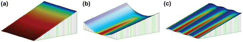
Figure 2 Schematic representation of a vegetated filter: (a) degree of submergence on vegetated filters, and (b) relative submergence as a function of Manning’s roughness coefficient (adapted from Wilson et al. 2005).

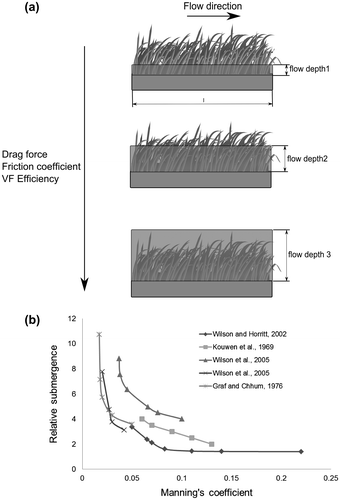
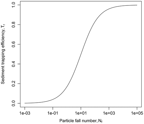
Figure 3 Sediment trapping efficiency as a function of particle fall number, derived from Deletic’s (2005) experiments.

Calculating sediment trapping efficiency with VFDM

VFDM follows a semi-empirical approach for estimating sediment trapping efficiency based on Deletic (2005), who proposed a semi-empirical model based on the assumption that sediment passing through a vegetated zone (q_s,out) depends on sediment inflow, vegetated filter width, particle size and density, and flow conditions. Translating the last paragraph into mathematical language, one obtains:(3) where q_s,out is the sediment outflow rate calculated as a function of vegetated filter width (l), flow velocity (V), flow depth (h), particle fall velocity (V_s) and sediment inflow rate (q_s,in). By applying the Buckingham theorem to Equation (3), Deletic (2005) derived the sediment trapping efficiency (T_r) for a uniformly vegetated filter as:(4) Deletic (2005) combined the non-dimensional parameters of Equation (4) into a new non-dimensional parameter called the particle fall number (N_f), given by:(5)

N_f expresses the ratio between the horizontal travel time and the vertical travel time of a sediment particle in suspension. Deletic (2005) calculated flow velocity (V) as follows:(6) where q is the flow rate per unit of hillslope width (m² s^–1) and B₀ is the vegetation density (–). Equation 6 was modified for VFDM in order to account for channelization related to concentrated flow in erosion rills. Q_day is the mean daily flow rate per unit of hillslope width in (m² s^–1) :(7)

Instead of taking the flow rate per unit of hillslope width, the flow rate is calculated for the duration of a given rainfall event during which erosion takes places (RainTime), divided by the number of erosion rills on the hillslope (NRILL). This approach adapts the particle fall number (N_f) to specific flow conditions that apply in erosion rills. The settling velocity of sediment particles (V_s) is calculated as:(8) where g is the gravitational acceleration (m s^–2), the kinematic viscosity of water (), water density (), density of suspended matter (), and d_s particle diameter (m).Based on results from flume experiments with vegetated filters made of real grass, Deletic (2001) and Deletic and Fletcher (2006) proposed an empirical relationship between the particle fall number and sediment trapping efficiency (T_r), calculated as (Deletic 2005):(9)

By comparing Equation (6) to the new equation for flow rate in erosion rills Equation (7), it is clear that the sediment trapping efficiency calculated from the particle fall number depends directly on the average flow rate during the rainfall event causing erosion and the number of erosion rills per hillslope. The coefficient of determination (R²) for simulated sediment trapping efficiency with respect to measured trapping efficiency was as high as 0.85 (Deletic 2005). (Deletic 2001, 2005) noted that the approach based on the particle fall number is only valid for low sediment concentrations that do not influence sediment deposition, and does not account for the influence of runoff reduction on sediment trapping. As Deletic’s (2005) equation is empirically derived, it is valid for the range of measured unit discharges; in this case between 0 and 1.17 m s^–1, when unit discharge exceeds this value, VFDM assumes a user defined maximal RVFS width. The equations for sediment trapping efficiency were developed for saturated soils.

Calculating vegetated filter width using VFDM

The three-step procedure for calculating VF width in VFDM begins with the selection of a desired sediment trapping efficiency (T_r). A comparative study showed that typical sediment trapping efficiency varies between 24–100% (Gumiere et al. 2011a). Given that 0 < T_r < 1, VF width l can be derived from Deletic’s (2005) Equations (4), (5) and (6):(10)

The second step involves the calculation of flow depth h using Manning’s equation, solved iteratively using the Newton-Raphson method, which is formulated as follows:(11) where h₀ is an arbitrary flow depth, starting from which the Newton-Raphson algorithm calculates progressively better estimates of the flow depth (h) passing through the vegetation cover for a given flow rate until a convergence threshold is reached, W is the rill width, n is Manning’s roughness coefficient, and S the slope. It is noteworthy that in this version of VFDM vegetation is considered never submerged by the flow. The above equation is based on a simplified rectangular rill profile.

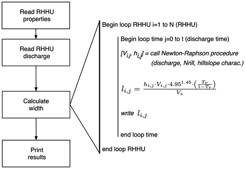
The last step in the procedure is the calculation of vegetated filter width corresponding with simulated hillslope runoff, in order to obtain the distributed vegetated filter width for all hillslopes. Figure 4 shows a schematic representation of the three-step approach discussed above.

Figure 4 Schematic representation of the algorithm used in the Vegetated Filter Dimensioning Model (VFDM) for calculating vegetated filter width. RHHU, relatively homogeneous hydrological unit.

Link with the HYDROTEL model for simulating runoff

VFDM was integrated into the GIBSI modeling platform in order to link the calculation of vegetated filter efficiency to the hydrological model HYDROTEL and the landscape discretization tool PHYSITEL. HYDROTEL is a process-based, distributed, continuous-time model for simulating runoff at the watershed scale (Fortin et al. 2001a; Turcotte et al. 2003; Turcotte et al. 2007; Bouda et al. 2012). As previously mentioned, it is based on the spatial subdivision of a watershed into relatively homogeneous hydrological units (RHHUs) and interconnected river segments (RSs) draining these RHHUs. A GIS-based framework called PHYSITEL (Turcotte et al. 2001; Rousseau et al. 2011) allows for a semi-automatic, spatial subdivision of the watershed and in turn facilitates parameterization of the hydrological objects (RHHUs and RSs).

HYDROTEL has six computational modules, which run in sequence. Each module simulates a specific hydrological process. In the first module, meteorological variables including liquid or solid precipitation, minimum and maximum temperatures, relative humidity, wind speed, and solar irradiance or insolation, are interpolated for each RHHU, with due care for vertical gradients if desired, using either Thiessen polygons or weighted means of the three nearest weather stations. The second module is the snow module. It simulates daily changes of mean snowpack characteristics (thickness, snow water equivalent, mean density, thermal deficit, liquid water content, temperature) using a modified energy budget-degree-day approach developed by Riley et al. (1972). The third module calculates the potential evapotranspiration (PET) for each RHHU using a choice of equations depending on available meteorological data, namely: (1) Thornthwaite (1948), (2) Linacre (1977); (3) Penman-Monteith (Monteith 1965); (4) Priestley and Taylor (1972); or (5) another equation developed by Hydro-Quebec. In the fourth module, the soil column moisture module, rainfall and/or snowmelt are partitioned into infiltration and runoff. For simulation purposes, the soil is subdivided into three horizontal layers. The surface layer is relatively shallow so as to correspond to the soil layer affected by evaporation over bare ground and to that, much smaller, layer for which soil moisture can be estimated by remote sensing. While the first layer controls infiltration, the second layer can be associated with direct flow and the third layer with base flow. In the current version of the model, the thicknesses of the three layers are assumed to be identical for all RHHUs or each RHHU cluster. Since the most sensitive model parameters are included in this module, it will be further explained in a following section. In the fifth module, which is the surface and subsurface flow routing module, the available amount of free water from each soil layer of RHHU is summed and routed to the corresponding downslope RS using an RHHU-specific geomorphological unit hydrograph (GUH). This hydrograph is determined once for each RHHU using the kinematic wave equation, but it can be recomputed when there is a change of land cover. The shape of the specific GUH is determined by routing a reference water depth over all DEM cells of a RHHU, according to the kinematic wave approach. The resulting values are considered as lateral inflow to the RS draining the RHHU. The sixth and last module is the channel routing module. Two simulation options are available: the diffusive and the kinematic wave equations, both being approximations of the Saint-Venant equation.

Link with the PHYSITEL landscape discretization tool

PHYSITEL is a landscape discretization tool for identifying drainage structure, hillslopes, sub-watersheds, physiographic databases and automatic parameterization of distributed hydrological models. Using a DEM, a soil map, a land cover map and, if available, a drainage network, the GIS computes parameters for RHHUs. Specifically, it determines internal drainage structure (slopes and local drainage direction), watershed boundaries, subwatershed and hillslope boundaries, and drainage network. The output of PHYSITEL can be used for a wide range of distributed hydrological models because of standard data formats and universal data types. The use of the D8-LTD algorithm (Orlandini et al. 2003) to compute the flow matrix and the optional use of a drainage network to determine the internal drainage structure of a watershed differentiate PHYSITEL from most GIS discretization tools. VFDM uses PHYSITEL to calculate flow convergence for each RHHU.

The United States Department of Agriculture (USDA 2000) noted that VF widths smaller than 0.5 m can be effective for pesticide trapping and that increasing width does not always improve trapping efficiency as a result of site-specific and runoff characteristics. In fact, the USDA (2000) describes techniques to promote shallow sheet flow across VFs, noting that concentrated flow is one of the primary factors limiting trapping efficiency. To account for this problem, VFDM introduces virtual channels or rills in the downslope direction, routing surface water and sediments from hillslope to river segments. PHYSITEL provides a method for determining the number of virtual rills intended to take into account the degree of flow channelization.

The method used to determine the degree of flow channelization is based on the assessment of plan shape and profile curvature characterizations developed by Noël et al. (2013), where a dominant flow direction is identified along with the left and right lateral hillslopes. The DEM is used to find contour lines and flow lines perpendicular to these contour lines in order to calculate plan shape and profile curvature, respectively. If the number of convex contour lines within a hillslope is larger than the number of concave contour lines, the hillslope is said to be convex. If there are as many convex contour lines as concave contour lines, the hillslope is said to be constant. Otherwise, it is said to be concave. An analogous procedure used to characterize the plan shape with elevation lines taken parallel to the average flow direction for a given river segment is calculated using the DEM. To characterize an elevation line as convergent, divergent or uniform, a straight reference line is drawn between the first and last cells of that elevation line. An elevation line is then designated as convergent if the majority of its cells fall far enough below the reference line, divergent if its cells fall far enough above the reference line, and uniform otherwise. The number of virtual erosion rills is now assumed to be between a user-specified maximum and minimum value related to maximum and minimum plan shape, respectively, between which the number of rills is linearly proportional to hillslope plan shape. VFDM seems to be very sensitive to the NRILL parameter; in fact, that is a well-known problem of predefined erosion rill models, such as MHYDAS-Erosion (Gumiere et al. 2011b). Future work of VFDM development includes the use of LIDAR images to assess erosion rills position and dimensions. Future work will involve performing a sensitivity analysis with respect to the resolution of the DEM.

Case study – Watershed application

Study site description

The Beaurivage River watershed

The Beaurivage River watershed was selected as the case study area. It is located in Quebec (Figure 5) and is representative of southern Quebec’s agricultural region. The Beaurivage River, with a length of 87 km and a drainage area of 718 km², is a tributary of the Chaudière River, which flows northwards into the Saint Lawrence River near Quebec City. Elevation ranges between 60 m at the watershed outlet and 663 m at the highest point on the southern tip.

Figure 5 (a) Location of the Beaurivage River watershed and two stream gauges, of which one is located 5 km upstream of the watershed outlet and one at the outlet of the Bras d’Henri subwatershed; (b)Land cover distribution; (c) Soil texture distribution.

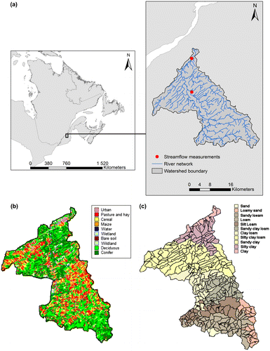
More than 34% of the watershed is used for agriculture, of which pasture occupies 82%, cereals (9%) and corn (8%) (Quilbé et al. 2006). The remainder is occupied by lakes (0.73 km²) and waterways (0.59 km²). Simoneau et al. (1998) observed phosphorus (P)-limited eutrophication of the water carried by the Beaurivage River, 86% of which they attributed to agricultural practice. Generous application of manure in the past has resulted in increased P concentrations in the soil, because P is less soluble than many of the other nutrients applied to the soil, such as nitrogen (N) (Simard et al. 1995).

Stream flow and water quality are monitored at the St. Etienne de Lauzon station, 5 km upstream of the outlet of the Beaurivage River watershed. For 2006–2008, the summer median concentration of total P varied between 0.051 to 0.100 mg/L (MDDEP 2012). Quilbé et al. (2006) estimated sediment and nutrient loads during the period 1989–1995 using the ratio estimator, and found relatively constant annual loads for dissolved N and P (on average 8.1 and 1.1 kg ha yr^–1, respectively), and a low erosion rate (0.23 t ha yr^–1). It is assumed that apart from agricultural pollution, the decline in water quality can partly be ascribed to point-source pollution resulting from untreated waste water (Bedard et al. 1998; Mailhot et al. 2008). More details about the Beaurivage River watershed can be found in Rousseau et al. (2013).

Implementation of vegetated filter strips

The Beaurivage River watershed is being studied as part of the multi-disciplinary WEBs project, which stands for Watershed Evaluation of Beneficial Management Practices. WEBs was launched in 2004 by Agriculture and Agri-Food Canada with the Canadian government and Ducks Unlimited Canada as the main funding partners, in order to quantify the effects of selected BMPs on economy and water quality. Since its conception, WEBs has raised the interest of many scientific partners (including Institut National de la Recherche Scientifique [INRS], University of Guelph, University of New Brunswick, University of Victoria, University of Alberta and many other institutes), and ongoing research involves nine agricultural watersheds across Canada.

Because of intensive animal husbandry in the Beaurivage River watershed (or its Bras d’Henri contributing subwatershed, to be more precise), this watershed was identified as playing a key role in the water quality of the Chaudière River (Lemelin 2008). Erosion by water was reported to cause several unwanted effects, such as reduced soil fertility, loss of agricultural land in close proximity to streams, sedimentation in streams and resulting maintenance costs, reduced accessibility for machines due to the presence of erosion rills, and a decrease in animal habitats and thus biodiversity. To study how these issues can be remedied, a number of anti-erosion measures were implemented at the microwatershed scale (drainage area of approximately 3 km²), including filling rills with stones and rocks, installing trenches, and creating grassed waterways and vegetated filter strips. The vegetated filter strips, with a width of up to 3 m, were applied as BMPs along the streams in the micro-watershed over a length of 6.7 km. They were subsequently planted with grass and shrubs like white cedar (Thuja occidentalis), viburnum (Viburnum trilobum) and broad-leaved meadowsweet (Spiraea latifolia).

Model parameterization

Model input

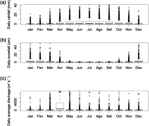
The hillslope runoff used as input for VFDM was provided by HYDROTEL, which was discretized into 1502 hillslopes, and calibrated a priori by Isabelle et al. (2011) with respect to discharge observed at the Beaurivage River watershed outlet during the period of 1 October 1969 to 30 September 2009, according to the procedure described by Turcotte et al. (2003). Most rainfall was measured during the summer (Figure 6), but discharge was highest in April during snowmelt. Lowest discharge was observed in January when almost no rainfall occurred. Precipitation was 875 mm on average, of which 250 mm was solid precipitation.

Figure 6 Precipitation and daily averaged stream flow in the Beaurivage River watershed used as input for the Vegetated Filter Dimensioning Model (VFDM); (a) rainfall, (b) snowfall, and (c) main outlet discharge (all data presented are for the 1969–2009 period).

Distributed model parameters

Due to the physical basis and distributed nature of VFDM, it is possible to provide for each hillslope a unique value for most parameters, including surface slope, Manning’s roughness coefficient, number and width of virtual erosion rills, vegetation density, runoff and sediment trapping efficiency of the vegetated filter. For this case study, we limited the number of distributed parameters to three: slope, number of virtual erosion rills and runoff.

The surface slope used to calculate flow depth and hillslope plan shape was derived from a DEM with a 25-m resolution. Hillslope plan shape was subsequently used to determine the number of virtual erosion rills per hillslope, which we assumed was equal to 1 for the greatest plan shape (convergent hillslope) and equal to 10 for the least plan shape (divergent hillslope). The number of rills was assumed to be linearly proportional to plan shape for values between greatest and least plan shape. It must be noted that the hillslopes in the Beaurivage River watershed are all convergent, which translates into a positive value for plan shape.

Hillslope runoff was simulated with HYDROTEL for the period 1 October 1969 to 30 September 2009, with a fairly good Nash-Sutcliffe coefficient of 0.76 with respect to flow measurements at the outlet of the Beaurivage River watershed.

Lumped model parameters

For the other parameters, lumped values were used. Manning’s roughness coefficient was set to 0.035, which is the value for cultivated floodplains with mature row crops (Chow 1959). The rill width used to calculate the depth of concentrated flow was set to 0.5 m for all rills; this value is based on field observations for the Beaurivage watershed.

The settling velocity for suspended sediment was calculated using a gravitational acceleration of 9.81 (m s^–2), kinematic viscosity of water of 1 10^–3 kg s^–1 m^–1, water density of 1 × 10³ kg m^–3, density of suspended matter of 2.6 × 10³ kg m^–3, and a particle diameter of 1 × 10^–4 m, the latter two values are characteristic of very fine sand.

It was assumed that the erosive force of hillslope runoff was applied during rainfall events of 12 hours, which is represented by a RainTime value of 12 by which daily simulated hillslope runoff was divided (Equation 7). The RainTime parameter may be estimated using frequency analyses of rainfall event time; the RainTime of 12 hours was chosen only for model testing and has no real significance.

Results and discussion

In this section, the VFDM results of the case study are discussed. This involved a 40-year runoff simulation (October 1969 to October 2009) for the Beaurivage River watershed generated by HYDROTEL. A vegetation density (B₀) between 0.5 and 0.8 was used, allowing a sediment trapping efficiency (T_r) between 0.6 and 0.8 in order to illustrate the effect of these parameters on the calculated RVFS width. Figure 7 shows the sediment trapping efficiency calculated with Deletic’s (2005) Equation (Equation 4) and 40 years of hydrological simulations for the Beaurivage watershed. The sediment trapping efficiency was calculated using fixed RVFS widths of 1.0, 3.0 and 5.0 m (Figure 7a, b and c) over all RHHUs (in this case, hillslopes). Calculated sediment trapping efficiency for 1.0, 3.0 and 5 m varied between 0 and 0.8. Upstream hillslopes tend to have low sediment trapping efficiencies when compared to those of hillslopes near the watershed outlet; this may be explained by the high density of forest in this area, which has relatively low or very little runoff production.

Figure 7 Sediment trapping efficiency of Beaurivage watershed calculated within Deletic’s (2005) equation (Equation 4) and 40 years of hydrological simulations from HYDROTEL.

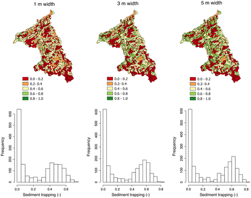
Table 1. List of parameters in the Vegetated Filter Dimensioning Model (VFDM) and sources for the parameterization.

Parameter	Description	Units	Source
S	Slope	(−)	PHYSITEL, DEM, LIDAR
n	Manning’s roughness coefficient	s m–1/3	Observations, remote sensing data
NRILL	Number of virtual erosion rills	(−)	Observations, PHYSITEL, DEM LIDAR
W	Width of virtual erosion rills	(m)	Observations, PHYSITEL, DEM, LIDAR
B0	Vegetation density	(−)	Observations, remote sensing
Q	Hillslope runoff	(m^3 day^–1)	HYDROTEL, discharge measurements
RainTime	Duration of rainfall event	(hours)	Meteorological data, frequency analyses
Tr	Sediment trapping efficiency of the vegetated filter	(−)	Literature or expert estimations
ds	Particle size	(μm)	Soil map, texture, aggregate stability tests

Figure 8 shows that T_r has a strong effect on calculated RVFS width, whereas the effect of B₀ is minimal. In fact, Figure 8 shows that the trapping efficiency, T_r, has a strong influence on RVFS width, whereas B₀ has a minimal influence in width calculation. In fact, the B₀ parameter is a type of correction factor used to take into account the effect of flow restriction over the hydraulic energy of the flow. Dunkerley (2002) has shown experimentally, using small wood blocks, that the water surface could rise 7 to 9 mm above the surface water; this could be explained by the influence of water surface tension.

Figure 8 Vegetated Filter Dimensioning Model (VFDM) simulated results of cumulative frequency of riparian vegetated filter strip (RVFS) widths over Beaurivage watershed, (a), (b), (c) and (d) correspond to B₀= 0.5, 0.6, 0.7, and 0.8, respectively (vertical dot lines represent the average values for RVFS width for the corresponding T_r grey tone).

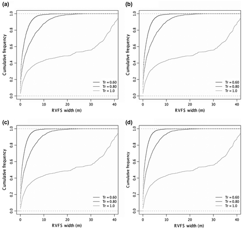
Table 2. Performance of the runoff simulation for the Beaurivage River watershed with respect to the period 1 October 1969 to 30 September 2009.

Metric	Watershed outlet
Nash-Sutcliffe	0.76
RMSE (m^3 day^–1)	11.71
R	0.88
R^2	0.77

In Table 3, the mean and the median value for RVFS width simulations are presented for the entire watershed. A T_r = 1.0 is not a realistic value, because it can be expected that some sediment passes through the vegetated filter; it is presented here for model stability check only. Values of RFVS simulated with VFDM are of the same order of magnitude as those that have been proposed by American and Canadian guidelines (Lee et al. 2004). The difference is that in VFDM, the widths are calculated based on the outflow of hillslopes and not on the river type. A non-statistically significant difference between mean RVFS widths is found for B₀ variation. However, the difference between RVFS widths related to T_r variation is statistically significant (p-value < 0.05). This result suggests that RFVS is very sensitive to T_r variation, implying that T_r is a user (or regulation) value that must be chosen carefully. For example, an increase of 17% in T_r produces an increase in the RVFS mean width of 145% for the same B₀ value.

Table 3. Results for the Vegetated Filter Dimensioning Model (VFDM) riparian vegetated filter strip (RVFS) width simulations.

	B0 = 0.5		B0 = 0.6		B0 = 0.7		B0 = 0.8
Tr	mean	median	mean	median	mean	median	mean	median
0.6	1.66	0.8	1.46	0.69	1.31	0.61	1.18	0.54
0.7	4.06	2.13	3.66	1.88	3.34	1.74	3.09	1.59
1.0	20.1	21.7	20.1	21.7	20.1	21.7	20.1	21.7

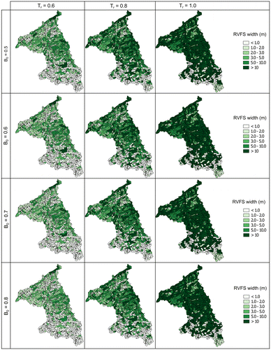
Figure 9 shows the simulated mean RVFS width for the Beaurivage watershed using VFDM and HYDROTEL hydrological simulations. It is noted that when the filtration threshold T_r is 0.6, RVFS widths tend to be reduced and only a few hillslopes require RVFS widths greater than 10 m. Similarly, when T_r is 0.8, almost the entire Beaurivage watershed requires a RVFS width greater than 10 m. For upstream hillslopes, the calculated mean RVFS widths are often less than 1.0 m; this can be explained because these hillslopes are essentially occupied by forest and they have relatively low runoff production when compared to an agricultural hillslope. Agricultural hillslopes are concentrated in the middle of Beaurivage watershed; it is noted that RVFS widths for this area are often between 5 and 10 m.

Figure 9 Optimized riparian vegetated filter strip (RVFS) width for Beaurivage watershed for three and four T_r (0.6, 0.8, 1.0) and B₀ (0.5, 0.6, 0.7, 0.8) values, respectively.

Conclusion

The vegetative riparian buffer guidelines are often based on water body type, shorelines, water body size and presence of fish. Some guidelines such as those of southeast, northeast, and mid-west regions of North America are “one size fits all” whereby a width is chosen and applied to the entire watershed. Other regions have adopted more complicated management approaches for RVFS dimensioning, such as in the North American Pacific boreal region, including Alaska. None of the USA/Canada guidelines take into account runoff velocity or flow concentration or even hillslope discharge volume for width calculation for agricultural watersheds. In this paper, the development of VFDM (Vegetated Filter Dimensioning Model) is presented, a computational distributed model intended to determine the optimal dimensions of riparian vegetated filter strips (RVFSs) for sediment trapping. An example of its application is given for the Beaurivage watershed.

VFDM is able to optimize RVFS width for all hillslopes of a watershed by taking into account slope, vegetation height, vegetation density and species composition; flow characteristics such as runoff velocity, discharge volume, water height and diffuse/convergent flow; and sediment characteristics such as particle size, aggregation and concentration. The originality of VFDM is the ability to spatially calculate the RVFS width for each hillslope in the watershed, accounting for surface properties, slope, soil type and discharge. The model is coupled with PHYSITEL and HYDROTEL, a watershed discretization tool and a distributed, process-based, hydrological model, respectively, within the modeling platform GIBSI.

The application of VFDM at the Beaurivage watershed has shown that upstream hillslopes require RVFS widths of less than 1.0 m because of the low runoff generation in these areas which is characterized by high concentration of forests in these parts of the watershed. For the Beaurivage watershed, the optimized RVFS width is between 5 and 10 m for agricultural hillslopes; these hillslopes are mostly concentrated in the middle of the watershed. The simulated RVFS widths have shown a high sensitivity to the sediment trapping threshold. Indeed, results have shown that 17% variation in T_r value may provide 145% variation in RVFS widths.

The next step for VFDM is the inclusion of an infiltration module which will be used to optimize RVFS widths for nutrients and pesticides. We are also working to include in VFDM transport and filtration equations, able to deal with a distribution of sediment sizes. The future development of VFDM includes: (1) use of LIDAR images for accessing erosion rill position and size and surface roughness parameters, (2) performing a sensitivity analysis with respect to the resolution of the digital elevation model and (3) linking the model to an economical model in order to evaluate the effectiveness of RVFSs with respect to both water quality and economic objectives.

Acknowledgements

This research was supported by the Watershed Evaluation of BMPs (WEBs) project, a partnership between Agriculture and Agri-Food Canada and Ducks Unlimited Canada. The authors wish to thank Shane Gabor of Ducks Unlimited Canada, and Brook Harker, David Kiely, Éric van Bochove, Georges Thériault and Terrie Scott of Agriculture and Agri-Food Canada for research coordination and collaboration. The authors also thank our colleagues at INRS-ETE, Sébastien Tremblay and Alain Royer, programmers, for their collaboration and Adriana Furlan for mapping work.

References

- Baptist, M. J., V. Babovic, J. R. Uthurburu, M. Keijzer, R. E. Uittenbogaard, A. Mynett, and A. Verwey. 2007. “On inducing equations for vegetation resistance.” Journal of Hydraulic Research 45 : 435–450.
- Barfield, B. J., E. W. Tollner, and J. C. Hayes. 1979. “Filtration of sediment by simulated vegetation I. steady-state flow with homogenous sediment.” Transactions of the American Society of Agricultural Engineers 22 (3): 540–548.
- Bedard, Y., S. Gariepy, and F. Delisle. 1998. Bassin versant de la rivière Chaudiere: l’activité agricole et ses effets sur la qualité de l’eau. Quebec City, QC: Ministère de l’Environnement et de la Faune du Québec and Saint-Laurent Vision 2000.
- Borin, M., M. Vianello, F. Morari, and G. Zanin. 2005. “Effectiveness of buffer strips in removing pollutants in runoff from a cultivated field in north-east Italy.” Agriculture, Ecosystems and Environment 105 : 101–114.
- Bouda, M., A. N. Rousseau, S. J. Gumiere, P. Gagnon, B. Konan, and R. Moussa. 2013. Implementation of an automatic calibration procedure for HYDROTEL based on sensitivity and identifiability analyses. Hydrological Processes doi:10.1002/hyp.9882.
- Bouda, M., A. N. Rousseau, B. Konan, P. Gagnon, and S. Gumiere. 2012. “Bayesian uncertainty analysis of the distributed hydrological model HYDROTEL.” Journal of Hydrologic Engineering 17 (9): 1021–1032.
- Cammeraat, L. H., and A. C. Imeson. 1999. “The evolution and significance of soil-vegetation patterns following land abandonment and fire in Spain.” CATENA 37 (1–2): 107–127.
- Chow, V. T. 1959. Open channel hydraulics. New York: McGraw-Hill.
- Cooper, J. R., J. W. Gillian, R. B. Daniels, and W. P. Robarge. 1987. “Riparian areas as filters for agricultural sediment.” Soil Science Society of America Journal 51 (2): 416–420.
- Daniels, R. B., and J. W. Gilliam. 1996. “Sediment and chemical load reduction by grass and riparian filters.” Soil Science Society of America Journal 60 : 246–251.
- Deletic, A. 2001. “Modelling of water and sediment transport over grassed areas.” Journal of Hygrology 248 (1–4): 168–182.
- Deletic, A. 2005. “Sedmient transport in urban runoff over grassed areas.” Journal of Hygrology 301 (1–4): 108–122.
- Deletic, A., and T. D. Fletcher. 2006. “Performance of grass filters used for stormwater treatment – A field and modelling study.” Journal of Hygrology 317 (3–4): 261–275.
- Dillaha, T. A., R. B. Reneau, S. Mostaghimi, and D. Lee. 1989. “Vegetative filter strips for agricultural nonpoint source pollution-control.” Transactions of the American Society of Agricultural Engineers 32 (2): 513–519.
- Dunkerley, D. 2002. “Surface tension and friction coefficients in shallow, laminar overland flows through organic litter.” Earth Surface Processes and Landforms 27 (1): 45–58.
- Fitzjohn, C., J. L. Ternan, and A. G. Williams. 1998. “Soil moisture variability in a semi-arid gully catchment: Implications for runoff and erosion control.” CATENA 32 (1): 55–70.
- Fortin, J. P., R. Turcotte, S. Massicotte, R. Moussa, J. Fitzback, and J. P. Villeneuve. 2001a. “A distributed watershed model compatible with remote sensing and GIS data. Part I: Description of model.” Journal of Hydrologic Engineering 6 (2): 91–99.
- Gumiere, S. J., Y. Le Bissonnais, D. Raclot, and B. Cheviron. 2011a. “Vegetated filter effects on sedimentological connectivity of agricultural catchments in erosion modelling: A review.” Earth Surface Processes and Landforms 36 : 3–19.
- Gumiere, S. J., D. Raclot, B. Cheviron, G. Davy, X. Louchart, J.-C. Fabre, R. Moussa, and Y. L. Bissonnais. 2011b. “MHYDAS-Erosion: A distributed single-storm water erosion model for agricultural catchments.” Hydrological Processes 25 (11): 1717–1728.
- Isabelle, P.-É., S. J. Gumiere, and A. N. Rousseau. 2011. Comparaison des calculs de la largeur optimale d’une bande riveraine par une approche mécaniste pour une division en sous-bassins et en versants. Rapport interne 1323. Québec, PQ: Centre Eau, Terre et Environnement, Institut national de la recherche scientifique (INRS-ETE).
- Järvelä, J. 2002. “Flow resistance of flexible and stiff vegetation: A flume study with natural plants.” Journal of Hydrology 269 (1–2): 44–54.
- Kouwen, N., and T. E. Unny. 1973. “Flexible roughness in open channels.” Journal of the Hydraulics Division 99 (5): 713–728.
- Lacas, J. G., M. Voltz, V. Gouy, N. Carluer, and J. J. Gril. 2005. “Using grassed strips to limit pesticide transfer to surface water: A review.” Agronomy for Sustainable Development 25 (2): 253–266.
- Lawrence, D. S. L. 1997. “Macroscale surface roughness and frictional resistance in overland flow.” Earth Surface Processes and Landforms 22 (4): 365–382.
- Le Bissonnais, Y., V. Lecomte, and O. Cerdan. 2004. “Grass strip effects on runoff and soil loss.” Agronomie 24 (3): 129–136.
- Lecomte, V. 1999. Transferts de produits phytosanitaires par le ruissellement et l’érosion de la parcelle au bassin versant. Modélisation spatiale. Ph.D. thesis, ENGREF et INRA-Orléans.
- Lee, P., C. Smyth, and S. Boutin. 2004. “Quantitative review of riparian buffer width guidelines from Canada and the United States.” Journal of Environmental Management 70 : 165–180.
- Lemelin, D. 2008. Aménagements hydro-agricoles microbassin versant dans le sous-bassin hydrographique Bras d’Henry de la rivière Chaudière. Évaluation des pratiques de gestion bénéfiques à l’échelle des bassins hydrographiques (EPB). Quebec City, QC: Ministère de l’Agriculture, Pêcheries et Alimentation du Québec.
- Linacre, E. T. 1977. “A simple formula for estimating evaporation rates in various climates, using temperature data alone.” Agricultural Meteorology 18 : 409–424.
- Lim, T. T., D. R. Edwards, S. R. Workman, B. Larson, and L. Dunn. 1998. “Vegetated filter strip removal of cattle manure constituents in runoff.” Transactions of the American Society of Agricultural Engineers 41 (5): 1375–1381.
- Magette, W. L., R. B. Brinsfeld, R. E. Palmer, and J. D. Wood. 1989. “Nutrient and sediment removal by vegetated filter strips.” Transactions of the American Society of Agricultural Engineers 32 (2): 663–667.
- Mailhot, A., A. N. Rousseau, G. Talbot, P. Gagnon, and R. Quilbé. 2008. “A framework to estimate sediment loads using distributions with covariates: Application to the Beaurivage River watershed (Quebec, Canada).” Hydrological Processes 22 (26): 4971–4985.
- Ministère du Développement durable, de l’Environnement et des Parcs (MDDEP). 2012. Portrait de la qualité des eaux de surface au Québec, 1999–2008. Direction du suivi de l'état de l’environnement: Ministère du Développement durable, de l’Environnement et des Parcs.
- Monteith, J. L. 1965. “Evaporation and environment.” Symp. Soc. Expl. Biol. 19 : 205–234.
- Nepf, H. M. 1999. “Drag, turbulence, and diffusion in flow through emergent vegetation.” Water Resources Research 35 (2): 479–489.
- Noël, P., A. N. Rousseau, C. Paniconi, and D. F. Nadeau. 2013. An algorithm for delineating and extracting hillslopes and hillslope width functions from gridded elevation data. Journal of Hydrologic Engineering doi: 10.1061/(ASCE)HE.1943-5584.0000783.
- Orlandini, S., G. Moretti, and M. Franchini. 2003. “Path-based methods for the determination of non dispersive drainage directions in grid-based digital elevation models.” Water Resources Research 39 (6): 1114.
- Priestley, C. H. B., and R. J. Taylor. 1972. “On the assessment of surface heat flux and evaporation using large scale parameters.” Monthly Weather Review 100 : 81–92.
- Quilbé, R., and A. N. Rousseau. 2007. “GIBSI : An integrated modelling system for watershed management – Sample applications and current developments.” Hydrology and Earth System Sciences 11 : 1785–1795.
- Quilbé, R., A. N. Rousseau, M. Duchemin, A. Poulin, G. Gangbazo, and J. P. Villeneuve. 2006. “Selecting a calculation method to estimate sediment and nutrient loads in streams: application to the Beaurivage River (Québec, Canada).” Journal of Hydrology 326 : 295–310.
- Riley, J. P., E. K. Israelsen, and K. O. Eggleston. 1972. “Some approaches to snowmelt prediction.” Actes du Colloque de Banff sur le Rôle de la Neige et de la Glace en Hydrologie, AISH 2 (107): 956–971.
- Rousseau, A. N., J. P. Fortin, R. Turcotte, A. Royer, S. Savary, F. Quévy, P. Noël, and C. Paniconi. 2011. “PHYSITEL, a specialized GIS for supporting the implementation of distributed hydrological models.” Water News 31 (1): 18–20.
- Rousseau, A. N., A. Mailhot, R. Quilbé, and J. P. Villeneuve. 2005. “Information technologies in the wider perspective: Integrating management functions across the urban-rural interface.” Environmental Modelling & Software 20 : 443–455.
- Rousseau, A. N., L. Paul, and C. Paniconi. 2007. A computational algorithm for hillslope partitioning from DEMs and digitized river networks. In AGU Fall Meeting, 10–14 December, 2007, ed. Eos Trans. San Fransisco, CA: Fall Meet. Suppl. Abstract H43G–1699.
- Rousseau, A. N., S. Savary, W. Hallema Dennis, S. J. Gumiere, and E. Foulon. 2013. Modeling the effects of agricultural BMPs on sediments, nutrients and water quality of the Beaurivage River watershed (Quebec, Canada). Canadian Water Resources Journal 38 (2): 99–120. doi:10.1080/07011784.2013.780792.
- Schmidt, J., M. Vvon Werner, and A. Michael. 1999. “Application of the EROSION 3D model to the CATSOP watershed, The Netherlands.” CATENA 37 (3–4): 449–456.
- Simard, R. R., D. Cluis, G. Gangbazo, and S. Beauchemin. 1995. “P status of forest and agricultural soils from a watershed of high animal density.” Journal of Environmental Quality 24 (5): 1010–1017.
- Spatz, R., F. Walker, and K. Hurle. 1997. Effect of grass buffer strips on pesticide runoff under simulated rainfall. Meded Fac Landbouwkd Toegep Biol Wet Univ Gent 799–806.
- Srivastava, P., D. R. Edwards, P. A. Daniel, P. A. Moore, and T. A. Costello. 1996. “Performance of vegetative filter strips with varying pollutant source and filter strip lengths.” Transactions of the American Society of Agricultural Engineers 39 (6): 2231–2239.
- Syversen, N., and H. Borch. 2005. “Retention of soil particle fractions and phosphorus in cold-climate buffer zones.” Ecological Engineering 25 (4): 382–394.
- Thornthwaite, C. W. 1948. “An approach toward a rational classification of climate.” Geographical Review 38 : 55–94.
- Tingle, C. H., D. R. Shaw, M. Boyette, and G. P. Murphy. 1998. “Metolachlor and metribuzin losses in runoff as affected by width of vegetative filter strips.” Weed Science 46 : 475–479.
- Turcotte, R., L. G. Fortin, V. Fortin, J. P. Fortin, and J. P. Villeneuve. 2007. “Operational analysis of the spatial distribution and the temporal evolution of the snowpack water equivalent in southern Québec, Canada.” Nordic Hydrology 38 (3): 211–234.
- Turcotte, R., J. P. Fortin, A. N. Rousseau, S. Massicotte, and J. P. Villeneuve. 2001. “Determination of watershed drainage structure using a digital elevation model and a digital river and lake network.” Journal of Hydrology 240 : 225–242.
- Turcotte, R., P. Lacombe, C. Dimnik, and J. P. Villeneuve. 2004. “Distributed hydrological prediction for the management of Quebec’s public dams.” Canadian Journal of Civil Engineering 31 (2): 308–320.
- Turcotte, R., A. N. Rousseau, J. P. Fortin, and J. P. Villeneuve. 2003. “A process-oriented multiple-objective calibration strategy accounting for model structure.” In Calibration of watershed models, edited by Q. Duan, V.K. Gupta, S. Sorooshian, A.N. Rousseau, and R. Turcotte, 153–163. Washington, DC: American Geophysical Union.
- United States Department of Agriculture (USDA). 2000. Conservation buffers to reduce pesticide losses. Oregon: Natural Resources Conservation Service.
- Wang, X. H., C. Q. Yin, and B. Q. Shan. 2005. “The role of diversified landscape buffer structures for water quality improvement in an agricultural watershed, North China.” Agriculture, Ecosystems and Environment 107 (4): 381–396.
- Wilson, C. A. M. E., T. Stoesser, and P. D. Bates. 2005. Modelling of open channel flow through vegetation CH.15 In Computational fluid dynamics: Applications in environmental hydraulics, ed. P. D. Bates, S. N. Lane and R. I. Ferguson, Ltd., Chichester, UK: John Wiley and Sons.
- Wu, F. C., H. W. Shen, and Y. J. Chou. 1999. “Variation of roughness coefficients for unsubmerged and submerged vegetation.” Journal of Hydrologic Engineering 9 (9): 934–942.
- Young, R. A., T. Huntrods, and W. Anderson. 1980. “Effectiveness of vegetated buffer strips in controlling pollution from feedlot runoff.” Journal of Environmental Quality 9 (3): 483–487.