The 2005 flood events in the Saskatchewan River Basin: Causes, assessment and damages

Abstract

In June 2005, the headwater tributaries of the Saskatchewan River Basin in the western Canadian province of Alberta were struck by four heavy rain events. Runoff from the rainfalls resulted in three floods which extended from Alberta through the provinces of Saskatchewan and Manitoba, causing at least four deaths and property damages of CAD $400 million.

En juin 2005, les affluents situés dans la partie en amont du bassin versant de la rivière Saskatchewan dans l’ouest du Canada (plus spécifiquement en Alberta), ont reçu de très importantes quantités de pluie durant quatre événements successifs. Le ruissellement causé par ces précipitations est à l’origine de trois crues, qui se sont produites en Alberta, en Saskatchewan et au Manitoba. Ces événements ont causé au moins trois décès et des dommages structurels évalués à 400 millions $CAD.

Geographical and hydrological setting

The Saskatchewan River Basin has a gross area of about 372,000 km² and extends from the Rocky Mountains of Alberta through Saskatchewan to Manitoba, as shown in Figure 1. The two main tributaries are the North and South Saskatchewan Rivers, with gross drainage areas of approximately 140,000 and 169,000 km², respectively. The main tributaries of the South Saskatchewan River are the Oldman, the Bow and the Red Deer Rivers.

Figure 1. Saskatchewan River basin and major sub-basins.

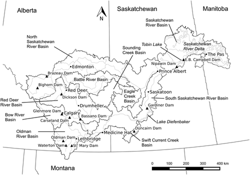
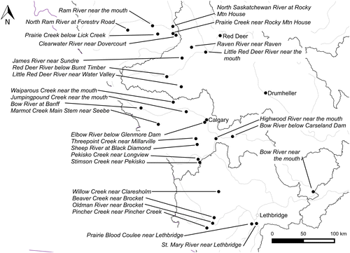
The Saskatchewan River is highly regulated for hydroelectricity, water supply (industrial, municipal and irrigation) and flood control. The locations of the major dams within the basin are shown in Figure 1. The Oldman and Red Deer rivers have large dams owned by the Government of Alberta, which can act to mitigate floods, as does the Gardiner Dam on the South Saskatchewan River, which is owned by the Government of Saskatchewan. The Bow and North Saskatchewan rivers have privately owned dams, which are not operated to control floods. However, the reservoirs of the Brazeau and Bighorn dams on the North Saskatchewan River did not experience very high inflows in the summer of 2005. There are also two hydroelectric dams (Nipawin and E. B. Campbell) on the Saskatchewan River near Nipawin, Saskatchewan. The locations of the headwater stream gauges selected for analysis are plotted in Figure 2.

Figure 2. Headwater stream gauges selected for analysis.

Causes of the floods

Antecedent conditions

In the spring of 2005, the drought which had affected the Canadian Prairies since 1999 (Hanesiak et al. 2011) was expected to continue. In May, mountain snow water equivalent (SWE) values were designated as being very low in the Oldman, Bow, Red Deer, North Saskatchewan and Athabasca River headwaters, due in part to early melting (Alberta Environment 2005a). Fall precipitation was generally designated as below normal in southern Alberta, although fall soil moisture (as modelled by Alberta Agriculture) was generally designated as being normal to above normal in the foothills (Alberta Environment 2005b).

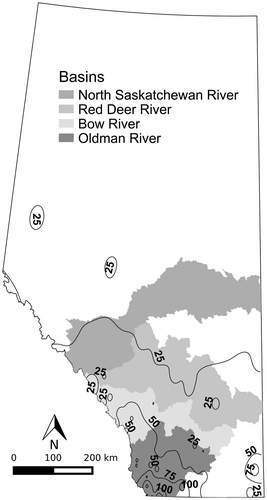
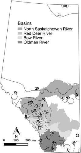
The three floods were directly preceded by a heavy rainfall event on 1–4 June, which deposited up to 150 mm of precipitation over a very large region of southern Alberta, with the greatest accumulations occurring in the extreme southwest, as shown in Figure 3. This event acted as a primer for the three floods by wetting the soils and increasing the flows of streams in the region, although no overbank flooding occurred.

Figure 3. Isohyets of pre-flood event accumulated precipitation, 1–4 June 2005.

Principal flood processes

The three flood events, and the initial priming event, were typical of large-scale high streamflows in Alberta in that they were caused by runoff from heavy rainfall due to large-scale low-pressure systems. Whenever these systems have moisture feeding from the Gulf of Mexico, very high rainfalls can result (Brimelow and Reuter 2005). As is also typical in Alberta, the heaviest precipitation fell in the foothills and mountains. Flesch and Reuter (2012) demonstrated that about half of the precipitation accumulations in the first and second flood precipitation events – the other events not being analyzed – were due to orographic lift caused by upslope winds.

Flood 1

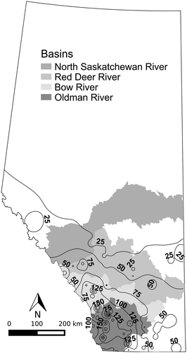
The precipitation causing the first flood event occurred over the interval 5–9 June. As shown in Figure 4, the heaviest precipitation, up to 253 mm, fell in the headwaters of the Oldman and Bow basins. In the upper Bow Basin, the heaviest precipitation fell in the southern portion.

Figure 4. Isohyets of the first flood event accumulated precipitation, 5–9 June 2005.

Flood 2

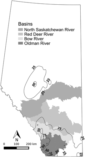
The second flood event was caused by up to 149 mm of precipitation falling over the interval 16–19 June. As shown in Figure 5, the greatest accumulations were in the upper Red Deer and North Saskatchewan basins.

Figure 5. Isohyets of the second flood event accumulated precipitation, 16–19 June 2005.

Flood 3

The third flood event was caused by up to 87 mm of precipitation that fell over 27–29 June. As shown in Figure 6, the heaviest precipitation fell in the Bow and Oldman basins.

Figure 6. Isohyets of the third flood event accumulated precipitation, 27–29 June 2005.

Statistical assessment

Statistical assessment of the 2005 events is complicated by the fact that up to three peaks were present on many streams; annual return periods only include a single event. Use of fitted distributions is further complicated by fact that annual peak streamflows in Alberta may be derived from snowmelt or from rainfall, which results in mixed frequency distributions. Furthermore, the flows on many of the streams in Alberta are strongly controlled by dams, as described above, as well as being influenced by diversions for cities and for irrigation. The total live storage upstream of each gauge in 2005 was estimated from the live storages for onstream reservoirs in Alberta (AMEC Environment & Infrastructure 2014) and Saskatchewan (Global Energy Observatory 2010, 2011). In many cases, the live storage upstream of a gauge has increased over the streamflow period of record as dams were constructed, further altering the distribution of peak flows. Because the Brazeau and Bighorn dams in the North Saskatchewan Basin were unaffected by the high flows during all three events, the live storages of their reservoirs were omitted from the North Saskatchewan stations. The estimated total live storages upstream of the selected gauges are shown in Table 1; all errors in the estimates are the responsibility of the author.

Table 1. Annual instantaneous peak flows for the floods of 2005, and their return periods, for stations in the Saskatchewan River Basin. Also shown are the total upstream live storage in 2005, the length of the record of peak flows and the last year for which a peak flow was available. Return periods for the floods of record, which are marked with an asterisk, were estimated using a fitted log-Pearson III distribution; all other return periods were estimated using the empirical cumulative distribution function (ECDF).

Basin and station	Station name	Upstream live storage(dam^3)	Last year in record	Record length(years)	Instant. peak flow(m^3/s)	Peak Date	Return period(years)	Ratio of 2005 peak flow to median peak
North Saskatchewan River Basin
05DB002	Prairie Creek near Rocky Mountain House	0	2011	52	212	19 June	73*	6.5
05DB005	Prairie Creek below Lick Creek	0	2011	34	275	18 June	536*	15
05DB006	Clearwater River near Dovercourt	0	2011	34	938	19 June	86*	12
05DC001	North Saskatchewan River near Rocky Mountain House	0	2011	59	2420	19 June	59	4.3
05DC006	Ram River near the mouth	0	2012	42	1124	18 June	65*	7.4
05DC011	North Ram River at Forestry Road	0	2011	36	75.2	18 June	20*	3.8
05EF001	North Saskatchewan River near Deer Creek	0	2013	48	2680	22 June	8	2.8
05GG001	North Saskatchewan River at Prince Albert	0	2013	61	1950	27 June	5	1.7
Red Deer River Basin
05CA002	James River near Sundre	0	2011	45	685	18 June	149*	13
05CA009	Red Deer River below Burnt Timber Creek	0	2011	35	1220	18 June	54*	8.1
05CB001	Little Red Deer River near the mouth	0	2011	31	452	19 June	48*	9.9
05CB002	Little Red Deer River near Water Valley	0	2012	43	614	18 June	124*	19
05CB004	Raven River near Raven	0	2011	30	90.5	19 June	347*	5.7
05CC002	Red Deer River at Red Deer	202,900	2013	57	1510	19 June	57	4.0
05CE001	Red Deer River at Drumheller	202,900	2011	42	1450	21 June	40*	3.3
05CK004	Red Deer River near Bindloss	227,365	2012	42	1050	23 June	25*	3.2
Bow River Basin
05BB001	Bow River at Banff	0	2011	63	174	23 June	1.4	0.8
05BF016	Marmot Creek Main Stem near Seebe	0	2011	49	2.02	18 June	10	2.0
05BG006	Waiparous Creek near the mouth	0	2012	46	240	18 June	76*	7.3
05BH004	Bow River at Calgary	672,500	2013	92	791	18 June	15	2.2
05BH009	Jumpingpound Creek near the mouth	0	2005	39	213	18 June	46*	8.7
05BJ001	Elbow River below Glenmore Dam	23,400	2012	37	301	19 June	101*	4.8
05BL007	Stimson Creek near Pekisko	0	2011	50	135	7 June	60*	9.7
05BL013	Threepoint Creek near Millarville	0	2012	40	389	17 June	38*	10
05BL014	Sheep River at Black Diamond	0	2012	42	380	7 June	30*	7.0
05BL023	Pekisko Creek near Longview	0	2011	42	119	7 June	31*	8.9
05BL024	Highwood River near The Mouth	0	2011	38	1340	18 June	46*	7.9
05BM002	Bow River below Carseland Dam	695,900	2011	55	1980	18 June	56*	4.0
05BN012	Bow River near the Mouth	695,900	2013	42	1640	20 June	42	3.3
Oldman River Basin
05AA004	Pincher Creek at Pincher Creek	0	2011	50	99.5	7 June	25	5.9
05AA024	Oldman River near Brocket	490,180	2012	45	1110	8 June	45	3.9
05AB013	Beaver Creek near Brocket	0	2011	35	48.3	7 June	19*	18
05AB021	Willow Creek near Claresholm	14,680	2011	43	694	7 June	68*	19
05AD035	Prairie Blood Coulee near Lethbridge	0	2011	30	63.1	8 June	30	13
05AE006	St. Mary River near Lethbridge	369,310	2011	81	421	8 June	16	3.7
South Saskatchewan River Basin
05AJ001	South Saskatchewan River at Medicine Hat	1,785,095	2013	66	3790	10 June	17	2.9
05HG001	South Saskatchewan River at Saskatoon	10,464,663	2013	53	1890	22 June	7	2.2
Saskatchewan River Basin
05KD003	Saskatchewan River below Tobin Lake	11,087,663	2013	32	2960	23 June	11	2.4

The annual peak flows were determined from the Water Survey of Canada HYDAT database of 17 July 2014 (Environment Canada 2014). Only stations having at least 30 years of data were selected for analysis. The dates and the magnitudes of the instantaneous peak flows, and the number of years analyzed, are listed in Table 1. The very large peak flows in the summer of 2013 will have altered the frequency distributions for many stations, but official values for the 2013 peaks were not yet available for some stations at the time of writing. The last year for which a peak flow was available is also listed for each station in Table 1.

Because of the limitations in the datasets, the frequency analyses included here used the non-parametric empirical cumulative distribution function (ECDF) (Wilk and Gnanadeskan 1968). The advantage of the ECDF is that it does not use a specified frequency distribution, which is likely to be invalid for the reasons discussed. A disadvantage of the ECDF is that it cannot give a return period for the flood of record. The ECDF-derived return periods for the peak flows other than the floods of record are listed in Table 1.

Return periods for the floods of record were estimated using log-Pearson III distributions fitted by L-moments using the R package “lmomco” (R Core Team. 2013). This distribution was selected because it provided a good fit for the majority of peak flows, as defined by their lying within the 95% confidence intervals, which were determined for each time series by bootstrapping. The return periods estimated from the fitted distribution should be treated with great caution, and are only given to characterize the rarity of the floods of record. Because of scatter in their fitting to the log-Pearson III distribution, the estimated return periods of some of the flows of record are shorter than the period of record. The log-Pearson III return periods are listed in Table 1, where they are marked with an asterisk.

To further illustrate the magnitude of each event, the instantaneous peak flow for 2005 for each station was divided by the median value of the peak flows for the period of record to produce the median peak flow ratio, which is listed for each station in Table 1. Some of the headwater stations had median peak flow ratios of 10 to 15. As flows progressed downstream, the magnitudes of the median peak flow ratios generally declined, reaching a value of 2.4 near the mouth of the Saskatchewan River.

Flood time course

The progress of the floods is shown by daily hydrographs of river flows and reservoir stages in Figures 7 through 18. All values were obtained from the Water Survey of Canada HYDAT database of 17 July 2014 (Environment Canada 2014). The hydrographs are discussed separately for each of the major sub-basins. The Alberta basins are listed from north to south. The North Saskatchewan, Red Deer and Bow basins are divided into upper (headwater) and lower reaches for clarity.

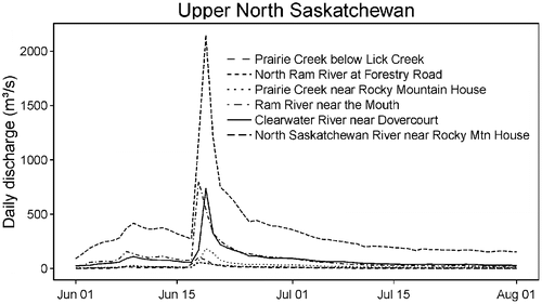
Figure 7. Hydrographs of mean daily discharges at stations in the upper North Saskatchewan River basin.

North Saskatchewan River Basin

As shown by the hydrographs plotted in Figure 7, the second flood was by far the largest of the three events in the upper reaches of the North Saskatchewan Basin, the first event producing negligible peaks and the third event producing no discernable peaks in the hydrographs. As described above and plotted in Figure 5, the heaviest second flood-event precipitation fell in the southern portion of the upper reaches of the basin, which were downstream of the Brazeau and Bighorn dams, whose locations are shown in Figure 1.

Many of the headwater tributaries (Prairie Creek, Ram, North Ram and Clearwater rivers) produced floods of record, with median peak flow ratios as large as 15. These high flows resulted in the peak streamflow at Rocky Mountain House having a return period of 59 years, and a median peak flow ratio of 4.3.

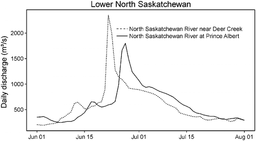
Figure 8 plots the flows on the lower reaches of the North Saskatchewan River. Although high flows were experienced on the North Saskatchewan River at Edmonton, there is no instantaneous peak flow available for 2005. The closest station to Edmonton is the North Saskatchewan at Deer Creek, which is located just west of the Alberta–Saskatchewan border. The peak flow at Deer Creek (2680 m³/s) was slightly larger than that at Rocky Mountain house (2420 m³/s), due to local inflows. The lack of contributions from the northern headwaters of the basin is clearly demonstrated by the return period of the Deer Creek peak being 8 years, and the corresponding median peak flow ratio being only 2.8, which were much smaller than at Rocky Mountain House. Further downstream at Prince Albert, the peak flow was reduced to 1950 m³/s, with a return period of 5 years and a median peak flow ratio of 1.7, by natural attenuation and the absence of local inflows.

Figure 8. Hydrographs of mean daily discharges at stations in the lower North Saskatchewan River basin.

Red Deer River Basin

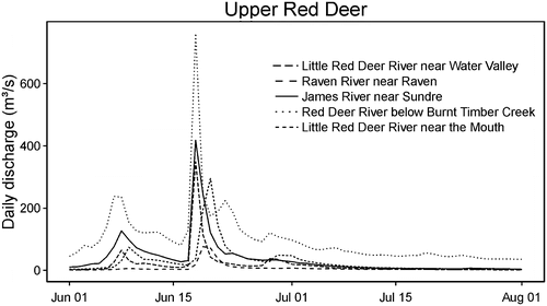
As with the North Saskatchewan Basin, the second flood event precipitation, plotted in Figure 5, was the largest of the three events in the headwaters of the Red Deer Basin and, consequently, the second event peaks of the headwater streams, as plotted in Figure 9, were the largest, resulting in flows of record on the James, Raven, Little Red Deer and Red Deer rivers. The large headwater flows resulted in very large inflows to the reservoir of the Dickson Dam, which is on the main stem of the Red Deer River above the city of Red Deer, as shown in Figure 1.

Figure 9. Hydrographs of mean daily discharges at stations in the upper Red Deer River basin.

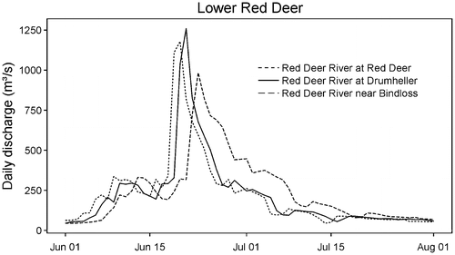
The hydrograph of the stage of the Dickson Dam reservoir (Glennifer Lake), which is plotted in Figure 10, shows evidence of a remarkable series of events. During the second flood event, the reservoir would likely not have filled to its full supply level (FSL). However, the very large peak flow on the Little Red Deer River (452 m³/s), which joins the Red Deer River downstream of the Dickson Dam, would have caused severe flooding downstream had the peak coincided with the dam’s peak discharge. To prevent this, the dam operators reduced the discharge, intentionally filling the reservoir to its FSL (the plot in Figure 10 shows the mean daily stage; the instantaneous peak elevation was essentially at the FSL), preventing the peak flows from coinciding. The quick action of the dam reduced the flood peak at Red Deer to 1510 m³/s. Through natural attenuation, the peak flow at Drumheller was reduced to 1450 m³/s, which is the flood of record, with a median peak flow ratio of 3.3. An emergency soil berm was constructed along the Red Deer River at Drumheller prior to the arrival of the flood peak. The combined effects of the shift in peak timing, flood wave attenuation and berm construction restricted the flooding mentioned in Table 2 to rural regions outside the berm. The hydrographs of daily flows (all that are available) on the lower Red Deer River plotted in Figure 11 do not show the attenuation of the instantaneous peak flow from Red Deer to Drumheller; however, the attenuation of the peak daily flow from Drumheller to Bindloss (1050 m³/s) is very evident.

Figure 10. Hydrograph of mean daily stage of Glennifer Lake, the reservoir of the Dickson Dam (solid line). The dashed line represents the full supply level (FSL) of the reservoir, which was obtained from http://www.environment.alberta.ca/apps/basins/woreport.aspx?wor=1546.

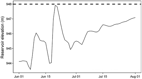
Table 2. Dates of peaks flows for flooded communities in Alberta.

Event	Community	Stream	Date of flood peak
Event 1	Pincher Creek	Pincher Creek	7 June
	High River	Highwood River	8 June
	Okotoks	Sheep River	7 June
	Medicine Hat	South Saskatchewan	10 June
Event 2	High River	Highwood River	18 June
	Okotoks	Sheep River	17 June
	Calgary	Elbow River	19 June
	Calgary	Bow River	18 June
	Red Deer	Red Deer	19 June
	Drumheller	Red Deer	21 June
Event 3	High River	Highwood River	28 June
	Okotoks	Sheep River	28 June

Figure 11. Hydrographs of mean daily discharges at stations in the lower Red Deer River basin.

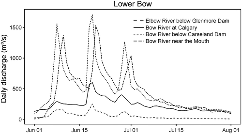
Bow River Basin

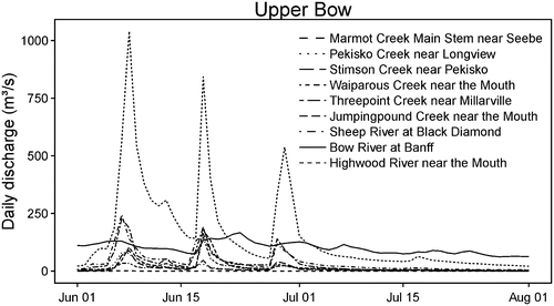
The upper reaches of the Bow Basin were hit by all three flood precipitation events, as shown in Figures 4, 5 and 6, resulting in three distinct peaks in the hydrographs of most of the streams in the basin headwaters, with the first event being the largest, as plotted in Figure 12. As described above, the heaviest rainfall missed the upper basin of the main stem of the Bow River in all three flood events, so the hydrograph of the Bow at Banff showed virtually no response to the first event, and only very muted responses to the other two, resulting in the return period of the peak flow of the Bow River at Banff being only 1.4 years, the median peak flow ratio being 0.8. The heavy precipitation in the foothills of the Bow Basin resulted in floods of record on a number of small creeks and rivers. Jumpingpound, Stimpson, Cataract and Pekisko Creeks, and the Elbow, Sheep and Highwood Rivers all had floods of record with median peak flow ratios as large as 10.

Figure 12. Hydrographs of mean daily discharges at stations in the upper Bow River basin.

The hydrographs of the lower reaches of the Bow Basin are plotted in Figure 13. The lack of high flows from the upper main stem of the Bow River contributed to the return period of the peak flow of the Bow at Calgary (791 m³/s) being only 15 years, with a median peak flow ratio of 2.2. The Water Survey of Canada (WSC) historical peak flows for the Bow at Calgary go back to 1915, but if the estimated historical peak flows for 1879 and 1897 (Neill and Watt 2001) are included in the analysis, then the return period is 12 years, with a median peak flow ratio of 2.1. The confluence of flows from more affected headwaters with those of the main stem resulted in a peak flow near the mouth of the Bow (1640 m³/s), which was only exceeded by the 2013 peak, and had a return period of 42 years and a median peak flow ratio of 3.3.

Figure 13. Hydrographs of mean daily discharges at stations in the lower Bow River basin.

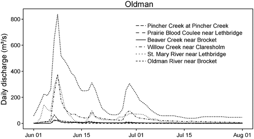
Oldman River Basin

The Oldman Basin was affected most strongly by the first flood rainfall event, as shown in Figure 4, which resulted in the peak flows for that event being the largest, as shown in Figure 14. The second and third flood rainfall events produced smaller peak flows whose magnitudes were very similar. Only two streams examined, Beaver Creek and Willow Creek, produced floods of record in the Oldman Basin, with median peak flow ratios of 18 and 19, respectively. Using the WSC data, which are missing a peak flow value for 1995, the peak flow of the Oldman River at Brocket had a return period of 45 years, with a median peak flow ratio of 3.9. However, when an estimated value of the 1995 flood peak of 3490 m³/s (Neill and Watt 2001) is added to the data set, then the return period is decreased to 23 years, the median peak flow ratio being 3.7.

Figure 14. Hydrographs of mean daily discharges at flows at stations in the Oldman River basin.

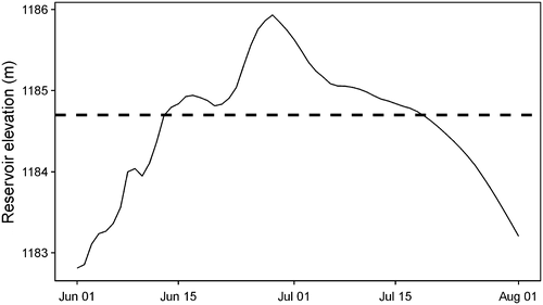
The four government-owned reservoirs in Alberta (Dickson, Oldman, Waterton and St. Mary) have established flood operating procedures. Each dam has a designated flood control pool, which is the difference between the current elevation and that required to pass its probable maximum flood (PMF) (Shook 2001). Thus, the reservoir elevation may exceed the FSL to reduce the downstream flooding, as occurred for the Oldman Dam in the first flood event, as shown in Figure 15, and for the Waterton Dam in the third, as shown in Figure 16. The St Mary’s reservoir did not exceed its FSL during the summer of 2005.

Figure 15. Hydrograph of mean daily stage of the reservoir of the Oldman Dam (solid line). The dashed line represents the full supply level (FSL) of the reservoir, which was obtained from http://www.environment.alberta.ca/apps/basins/woreport.aspx?wor=403.

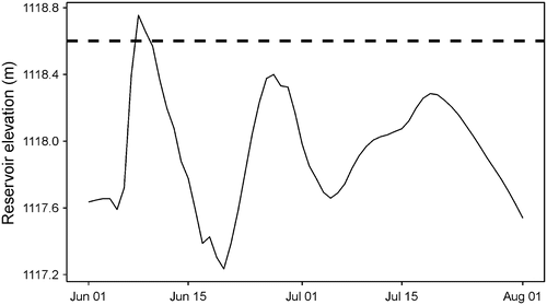
Figure 16. Hydrograph of mean daily stage of the reservoir of the Waterton Dam (solid line). The dashed line represents the full supply level (FSL) of the reservoir, which was obtained from http://www.environment.alberta.ca/apps/basins/woreport.aspx?wor=403.

South Saskatchewan Basin

The major tributaries (Oldman and Bow rivers) combined to produce very high flows on the South Saskatchewan River at Medicine Hat, where three flood peaks resulted, as plotted in Figure 17. The peak from the largest (the first) event (3790 m³/s) had a return period of 17 years, and a median peak flow ratio of 2.9. The flows on the Saskatchewan River combined with those on the Red Deer to produce the inflows to Lake Diefenbaker. The inflows from Swift Current Creek downstream of the Duncairn Dam (location shown in Figure 1) were negligible with a peak of 6 m³/s. Figure 18 plots the stage of Lake Diefenbaker over the duration of the floods. The decline in the reservoir elevation in early June occurred at the same time as the heavy precipitation of the first flood event, demonstrating that the reservoir’s operators took advantage of the routing time to increase the storage of Lake Diefenbaker prior to the arrival of the flood wave.

Figure 17. Hydrographs of mean daily discharges at flows at stations in the South Saskatchewan and Saskatchewan River basins.

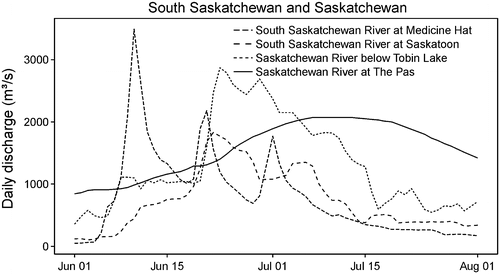
Figure 18. Hydrograph of mean daily stage of the reservoir of Lake Diefenbaker (solid line). The dashed line represents the full supply level (FSL) of the reservoir, which was obtained from www.wsask.ca/Lakes-and-Rivers/Dams-and-Reservoirs/Major-Dams-and-Reservoirs/Lake-Diefenbaker/.

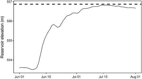
Apart from a period of drawdown after the first event, Lake Diefenbaker rose continually until it was very close to FSL on 14 July. Thus the reservoir mitigated the high inflows throughout all three flood events. The hydrograph of the South Saskatchewan River at Saskatoon in Figure 17 shows that the first, largest peak was almost completely removed. The second peak inflow was less attenuated, and resulted in a very broad peak at Saskatoon, where the return period of the peak flow (3790 m³/s) was 7 years, and the median peak flow ratio was 2.2. The reduced attenuation of the second peak was no doubt influenced by the reduction of available storage due to the first flood. However, Lake Diefenbaker is operated for many purposes other than flood control, including recreation, irrigation, power generation and wildlife preservation, which may also have influenced its operation. A fuller discussion of the constraints on the operation of Lake Diefenbaker is given by Centre for Hydrology (2012). The peak flow from the third flood event was also attenuated and broadened at Saskatoon.

Saskatchewan Basin

Farther downstream, the large peaks from the second flood event on the North and South Saskatchewan Rivers did not coincide, resulting in two peaks on the Saskatchewan River, as shown in Figure 18. The magnitude of the larger peak of the Saskatchewan River below Tobin Lake was 2960 m³/s with a return period of 11 years and a median peak flow ratio, due in part to attenuation by the action of the Nipawin and E. B. Campbell dams, as Tobin Lake was below its FSL throughout the summer of 2005. The hydrograph of the farthest downstream point, the Saskatchewan River at The Pas, in Figure 18, shows the strong attenuation of the peak flow (2070 m³/s) by the Saskatchewan River Delta, which was also noted by Smith and Pérez-Arlucea (2008).

Flood damages

Overbank flooding occurred in a number of Alberta communities on the dates listed in Table 2 (Alberta Environment 2005c). The city of Calgary was flooded by both the Bow and Elbow rivers, and the town of High River was flooded three times. Flooding was reported in communities in the Saskatchewan River Delta in Saskatchewan and Manitoba, and caused the village of Cumberland House to be evacuated.

The total cost of all of the 2005 floods has been estimated at CAD $400 million, and four deaths resulted (Flesch and Reuter 2012). In addition to the damage caused by the flooding, stress due to the severe disruption caused by the flooding adversely affected the mental health of farm families in the region (Acharya et al. 2007).

Summary

The high streamflows and floods in the summer of 2005 were the result of four large storms. The high streamflows persisted for very long periods of time downstream, particularly in Saskatchewan and Manitoba, because of the number of events, their large magnitudes and the effects of the dams on the rivers.

The destruction caused by the flooding in Alberta was largely due to historical development in the river flood plains. After the 2005 flood events, a committee composed of representatives from Alberta Infrastructure and Transportation (INFTRA), Alberta Environment (AENV) and Alberta Municipal Affairs (MA) issued 18 recommendations. Among these were that the flood risk maps for municipalities be updated, that crown lands no longer be sold in known flood risk areas, and that Flood Risk Management Guidelines for Location of New Facilities be followed for provincially-funded new facilities (Groeneveld 2006). Unfortunately, the recommendations of the report were not followed; the consequences were to be very apparent during the Alberta flooding in June 2013 (Pomeroy et al. this issue).

Acknowledgements

Financial support from Canada Research Chair, Natural Sciences and Engineering Research Council and the U of S Global Institute for Water Security is gratefully acknowledged. Precipitation data for all Alberta stations in June 2005 were supplied by Ralph Wright of the Alberta AgroClimatic Information Service (ACIS). The live storage data for Duncairn Reservoir were provided by Kevin Wingert, of the Saskatchewan Water Security Agency. All analyses were performed using Free Open Source Software (FOSS). All maps were created using QGIS, which is available at http://www.qgis.org/. All statistical analyses were performed using the language R (R Core Team 2013). The code for fitting the log-Pearson III distributions was based on an R script written by David Hutchinson of Environment Canada. All graphs were plotted in R using the package ggplot2 (Wickham 2009).

References

- Acharya, M. P., R. G. Kalischuk, K. K. Klein, and H. Bjornlund. 2007. Health impacts of the 2005 flood events on feedlot farm families in southern Alberta, Canada. In Water Resources Management IV, ed. C. A. Brebbia and A. G. Kungolos, WIT Transactions on Ecology and the Environment, Vol 103, I (May), 253–262. doi:10.2495/WRM070241. Southampton, UK: WIT Press.
- Alberta Environment. 2005a. Water supply outlook overview. http://www.environment.alberta.ca/forecasting/WaterSupply/may2005/overview_web.pdf ( accessed May, 2014).
- Alberta Environment. 2005b. Water supply outlook for Alberta, May 2005. http://www.environment.alberta.ca/forecasting/watersupply/may2005/mayTOC.html ( accessed May, 2014).
- Alberta Environment. 2005c. Review of June 2005 flood events in southern Alberta. Edmonton, Alberta. 16 pp.
- AMEC Environment & Infrastructure. 2014. Water storage opportunities in the South Saskatchewan River Basin in Alberta. Lethbridge, AB.
- Brimelow, J. C., and G. W. Reuter. 2005. Transport of atmospheric moisture during three extreme rainfall events over the Mackenzie River Basin. Journal of Hydrometeorology 6: 423–441.
- Centre for Hydrology. 2012. Review of Lake Diefenbaker operations 2010–2011. Centre for Hydrology final report to the Saskatchewan Watershed Authority. University of Saskatchewan, Saskatoon. 117 pp. http://www.usask.ca/hydrology/papers/Pomeroy_Shook_2012.pdf
- Environment Canada. 2014. HYDAT database. ftp://arccf10.tor.ec.gc.ca/wsc/software/HYDAT/ (accessed July, 2014).
- Flesch, T. K., and G. W. Reuter. 2012. WRF model simulation of two Alberta flooding events and the impact of topography. Journal of Hydrometeorology 13 (2): 695–708. doi:10.1175/JHM-D-11-035.1.
- Global Energy Observatory. 2010. E. B. Campbell Hydroelectric Generating Station. http://globalenergyobservatory.org/geoid/2998 ( accessed May, 2014).
- Global Energy Observatory. 2011. Nipawin Hydroelectric Generating Station Canada. http://globalenergyobservatory.org/geoid/4504 ( accessed May, 2014).
- Groeneveld, G. 2006. Provincial flood mitigation report: Consultations and recommendations. 32 pp. http://www.aema.alberta.ca/images/News/Provincial_Flood_Mitigation_Report.pdf ( accessed May, 2014).
- Hanesiak, J. M., R. E. Stewart, B. R. Bonsal, P. Harder, R. Lawford, R. Aider, B. D. Amiro, et al. 2011. Characterization and summary of the 1999–2005 Canadian Prairie Drought. Atmosphere-Ocean 49 (4): 421–452. doi:10.1080/07055900.2011.626757.
- Neill, C. R., and W. E. Watt. 2001. Report on six case studies of flood frequency analyses. Alberta Transportation and Civil Engineering Division Civil Projects Branch. http://www.transportation.alberta.ca/Content/doctype30/Production/ffasixcase.pdf ( accessed May, 2014).
- Pomeroy, J., R. E. Stewart, and P. H. Whitfield. 2015. The 2013 flood event in the Bow and Oldman River basins; causes, assessment, and damages. Canadian Water Resources Journal.
- R Core Team. 2013. R: A language and environment for statistical computing. Vienna, Austria: R Foundation for Statistical Computing. http://www.r-project.org/
- Shook, K. 2001. Waterton Dam flood operating procedures. Alberta Environment, Natural Resources Services, Water Management Division, Water Sciences Branch, Hydrology/Forecasting Section. 120 pp.
- Smith, N. D., and M. Pérez-Arlucea. 2008. Natural levee deposition during the 2005 flood of the Saskatchewan River. Geomorphology 101 (4): 583–594. doi:10.1016/j.geomorph.2008.02.009.
- Wickham, H. 2009. ggplot2: Elegant graphics for data analysis. New York, NY: Springer.
- Wilk, M. B., and R. Gnanadeskan. 1968. Probability plotting methods for the analysis of data. Biometrika 55 (1): 1–17. doi:10.1093/biomet/55.1.1.