A GIS-supported fuzzy-set approach for flood risk assessment

Abstract

This study presents a geographic information system (GIS)-supported three-dimensional fuzzy risk assessment approach (3D GIS-FRA) for flood risk assessment that is based on the development of a fuzzy-set risk model, 3D GIS mapping, and a hydro-statistical simulation. Using GIS and a digital elevation model (DEM), urban settings under different levels of flood risk are visualized and hydraulic simulations conducted for various river flow scenarios to determine the flow rates for specified risk levels. Then, a statistical analysis is carried out using historical records to establish a set of risk criteria that consider critical factors that affect the peak flow rate. Finally, the developed fuzzy-set risk model is applied to examine the flood risks using the outputs from the hydraulic models and statistical analysis. The developed method is applied to a section of the Red River in Southern Manitoba, Canada. The 3D GIS-FRA results indicate that there is a possibility of having a highly risky situation for the upper-bound extreme condition for the study area, although only limited impacts are expected for a 25-year flood. For the 75-year flood scenario, the overall flood risk level is high for the whole area. The results indicate that the developed risk analysis system is useful for systematically quantifying the flood risks and the related system uncertainties.

Abstract

Cet article présente une tridimensionnel évaluation des risques brouillée approche (3D SIG-FRA) basée sur le système d’information géographique (SIG) pour évaluer des risques d’inondation. L’étude s’est réalisée en développant un modèle de risque basé sur la théorie des ensembles et de la logique flous et à l’aide de la cartographie des données 3D provenant du SIG et de la simulation hydro-statistique. En utilisant le SIG et le model numérique d’élévation (MNE), l’environnement urbain à différents niveaux de risques d’inondation est visualisé, et des simulations hydrauliques sont menées pour divers scénarios d’écoulement de rivière dans le but de déterminer les débits correspondants à des niveaux de risques spécifiés. Ensuite, une analyse statistique est effectuée en utilisant les données historiques pour établir un ensemble de critères de risque dans lesquels les facteurs critiques affectant le débit de pointe sont considérés. Comme une autre étape, le modèle de risque développé en se basant sur l’ensemble flou est utilisé pour étudier les risques d’inondation à l’aide des résultats obtenus à partir des modèles hydrauliques et de l’analyse statistique. Enfin, la méthode développée est appliquée à une section de la rivière rouge qui se trouve dans le sud du Manitoba, Canada. Les résultats issus de la méthode proposée (3D GIS-FRA) indiquent qu’il y a une possibilité des situations à risque élevé sous conditions extrêmes pour le secteur à l’étude bien que seulement des incidences d’inondation limitées soient prévues pour une durée de 25 ans. En ce qui concerne le scénario d’inondation d’une durée de 75 ans, le niveau de risque global est élevé pour toute la région. Les résultats démontrent que le système d’analyse de risque développé est utile pour déterminer systématiquement les risques d’inondation et les incertitudes liées au système.

Introduction

The impacts of flooding are enormous since the development of civilizations is mainly river based (Heijne 1992). For example, during the flood in China in 1998, over 3000 people died, about 15 million were made homeless, and direct property damage was estimated at US $20 billion (Smith 2002). Similarly, in Canada, from 1993 to 1996, the nation experienced more than US $28 billion in losses and more than 300 people lost their lives due to floods (Pielke 1999). The number of events, the population affected by flooding events and the financial, economic and insured damages have all have risen rapidly over the period since 1950, as floods and storms are the major natural disaster in US and around the world (Jha et al. 2011). For instance, flood and storm-related impacts accounted for 77% of the major natural disasters in the US in 2009 (R.J. Chen 2011). Severe frequent flooding events also occurred in the Red River in the central part of North America in the twentieth century, and several studies have investigated flood risk in this river (e.g. Burn 1999; Haque 2000; Simonovic 2005; Ahmad and Simonovic 2011).

Flood forecasting and flood risk assessment are important tools for flood hazard mitigation. Generally, the assessment of flood risk consists of determining the probability of the occurrence and the degree of severity of floods at a given place. Assessment helps decision-makers to identify the most vulnerable areas and to develop both pre- and post-disaster mitigation strategies. Many studies have been undertaken on flood forecasting and management using various techniques including modelling, statistical and information technology methods. For instance, Rahman et al. (2002) used a Monte Carlo simulation technique to determine flood frequency curves. Todini (1999) developed an integrated method that combines geographic information systems (GIS) with mathematical models for flood management and planning. Chuntian (1999) introduced a fuzzy optimization model for flood control. For the Red River, Ahmad and Simonvic (2011) and Simonovic (2005) adopted fuzzy methodology for flood risk analysis.

In previous studies, statistical and fuzzy set methods have been used to quantify system uncertainties, showing that they are useful tools in environmental modelling. They avoid oversimplification and allow precise analysis and forecasting of complex, dynamic phenomena (Borri et al. 1998). Despite the applications of fuzzy set theory in a variety of engineering problems, applying the theory to flood risk management is a challenging task due to the difficulties in determining the objective membership functions and the complexity of solving the information duplication problem caused by related assessment indices (Liu et al. 2010). Still, researchers have developed or adopted the fuzzy set theory to assess the risk of dam safety and flood risk (Elmazoghi 2013).

Considering the large geographic extent of flood and flood-affected areas, GIS and high-resolution Digital Elevation Models (DEMs) are becoming fundamental tools for land use planning, flood management and natural hazard assessment. Abdalla et al. (2002) applied an integrated approach to assess flood risk based on GIS and hydraulic simulation. Lanza and Siccardi (1995) discussed the role of GIS as a tool for assessing flood hazard. Application of GIS in this field of study has expanded as three-dimensional (3D) visualization and spatial analysis are incorporated in the GIS tools (Kliskey and Byrom 2004). GIS has served as a powerful tool in risk assessment studies especially when coupled with other techniques.

A GIS-supported three-dimensional fuzzy risk assessment approach (3D GIS-FRA) is developed in the present study to assess flood risk and to quantify flood-induced impacts on urban areas. The method is applied to the Red River region in Southern Manitoba, Canada. This approach includes a fuzzy-set risk analysis model, a 3D GIS interface, a multi-regression analysis, a river simulation and flood risk mapping.

A 3D GIS-FRA approach for flood risk assessment

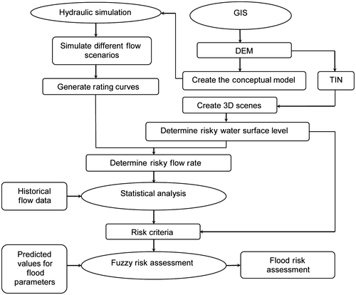
Figure 1 provides an overview of the 3D GIS-FRA approach which integrates four tools: hydraulic simulation, 3D GIS, statistical analysis and fuzzy set theory. First, a hydraulic simulation is conducted to establish the relationship between flow rates and water surface levels with high-resolution digital data. 3D GIS is then used to map flood impacts on the urban area as spatial risk criteria. Additionally, DEM and triangulated irregular network (TIN) models are used for both river system modelling and 3D GIS mapping. Statistical analysis is performed to determine the factors affecting the peak flow rate of the river chosen for the study. Outputs obtained from the hydraulic simulation and the statistical analyses are then used along with the historical data as inputs for the fuzzy risk assessment model to examine the flood risks, which are also represented in a 3D GIS.

Figure 1. Flow chart of flood risk assessment using 3D GIS-FRA (three-dimensional geographical information system fuzzy risk assessment approach). It integrates four functions: hydraulic simulation, 3D GIS including a digital elevation model and triangulated irregular network, statistical analysis, and fuzzy set theory.

Fuzzy risk model

Fuzzy set theory is a mathematical approach that addresses uncertainty arising from system complexity, incomplete information and imprecise human thought, language and perception (Leung 1988). To formulate the fuzzy risk model, two sets are defined (Z. Chen et al. 1998):(1a) (1b)

where U denotes a set of parameters or factors and V represents the set of risk levels. u_i represents parameter i, and v_j is for risk level j. A fuzzy subset of U can be determined using Equation (2(2) ), and a fuzzy subset of U × V, which is a binary fuzzy relation with U to V, can be characterized using Equation (3) to show a fuzzy relation matrix of m × n dimension.(2) (3a) (3b)

where a_i is the membership grade of u_i (for parameter i) and r_ij is the membership grade of parameter i versus the risk level j, which is a function of the parameter value and risk level criteria.

The integrated risk levels are calculated using Equations (4, 5, and 6(6) ) (Z. Chen et al. 1998; Zimmermann 2001):(4) (5) (6)

The model can be extended by considering the parameter values as interval values (Z. Chen et al. 1998) to quantify system uncertainties: (7)

where and are the lower and upper bounds of , respectively. When becomes a deterministic number. Since is fuzzy interval numbers, a parametric approach that improves Kuzmin’s method (Kuzmin 1981) is used to determine the membership functions for interval terms in . In Kuzmin’s technique, the membership is defined as a bilinear function using three parameters α, β and γ, where α < β < γ; α is the minimum value, and γ is the maximum value. Hence, the membership value of input factor p from fuzzy set A, denoted as , is equal to unity at β and zero at α and γ (Kuzmin 1981). can be expressed as follows:

when : (8a) (8b)

when :(9a) (9b)

when and :(10a) (10b)

Hence, the membership grade of the fuzzy relation between the given and the risk level j can be calculated as follows:

when : (11a) (11b)

when :(12a) (12b)

when or :(13)

when and :(14a) (14b)

where v_ij denotes the criterion for the parameter i contributing to the risk level j.

For a system involving several factors contributing to a risk or impact level, the integrated risks can be analysed using the modelling approach above. Assuming that a_i is the degree of significance for the factor i, and r_ij is the grade of membership for the fuzzy relation between the factor i and the risk level j, b_j, which represents the membership grade (possibility) for the integrated risk level j to occur, can be obtained through Equation (6).

Statistical analysis

A multiregression analysis model is developed in this section based on the historical information of the peak flow rates with the related data of: the Antecedent Precipitation Index (API) representing the soil moisture at freeze-up the previous autumn, based on weighted basin precipitation from May to October; Melt Index (MI) representing the water content of snowpack in terms of mean deg-days/day at Grand Forks during the active melt period; total winter precipitation (L) for the study area that is the total basin precipitation from November 1 of the previous year to the start of the spring crest at Emerson representing water content of snowpack; and the timing factor T, which is the percent of the worst possible south–north progression of melt snow and rain. These factors are well-identified important hydrological parameters contributing to a flood flow based on experience and flood studies. In particular, the timing factor has a major influence on flood peaks at the study area near Winnipeg. There are additional factors influencing the amount of runoff and flood peaks including soil frost depth, degree of clogging of ditches and tributaries with hard snow drifts or ice, spatial distribution of the soil moisture, snow cover and rainfall, rainfall intensities, etc. Although these parameters were not explicitly included in this study due to a lack of reliable associated historical data, their effects on major floods are assumed to be included implicitly through correlation with the four major selected parameters. The resulting model is that the flood flow rate or river surface level is a function of API, MI and L. This regression analysis is performed to obtain a standard flow simulation for a specific river basin under study and then to relate a flood level to a set of hydrological factors for that region.

In the developed 3D GIS-FRA, the statistical analysis is included to interpret the occurrence or return period of floods using a Log Pearson Type 3 distribution (Singh et al. 1986) as a supplement to the flood risk assessment, prior to the quantification of flood risks using the fuzzy-set risk model based on the obtained set of hydrological data.

Hydraulic simulation

For this study, the full one-dimensional (1D) Saint-Venant equations for unsteady open channel flow are solved using Hydrologic Engineering Centers River Analysis System (HEC-RAS) (Brunner 2001) to establish the dynamic relationship between the flow rate and the water surface level by considering different flow scenarios. The two basic equations are (Hoggan 1989):(15) (16)

where Y₁, Y₂ [L] are the depths of the water at cross sections, Z₁, Z₂ [L] are the elevations of the main channel inverts, V₁, V₂ [L/T] are the average velocities (total discharge/total flow area), a₁, a₂ are the velocity weighting coefficients, g [L/T²] is the gravitational acceleration and h_e [L] is the energy head loss: L [L] is the discharge weighted reach length, is the representative friction slope between two sections and C is the expansion or contraction loss coefficient. For this model, it is assumed that the river flow is under uniform flow conditions at the downstream boundary.

The distance weighted reach length, L, is given by the following:(17)

where, L_lob, L_ch, L_rob [L] are the cross section reach lengths and [L] are the arithmetic average of the flows between sections for the left overbank, main channel and right overbank, respectively.

GIS digital map and DEM data are used to improve the above hydraulic analysis by using an accurate analysis of river and floodplain geometry. ArcView GIS (ESRI 2011) is used for the data management and programming in the present study.

3D GIS

In the present study, the primary use of GIS is to visualize the topography of the study area, to classify the topography into different classes according to water surface level, to visualize the effects of different water surface levels on the flooded area, to determine the flood condition of the topography and, at the same time, to visualize the urban settings in three dimensions. This is undertaken by processing the DEM in the GIS interface to create a TIN, which facilitates the development of the risk maps. Also, GIS is used for pre- and post-processing steps for hydraulic simulation. For example, it supports the hydraulic simulation for the study area, which involves defining river reaches (layouts and attributes), the position of the cross sections of those reaches (orientations and station values), bank locations and flood zones.

Application of 3D GIS-FRA to the Red River

Overview of the study area

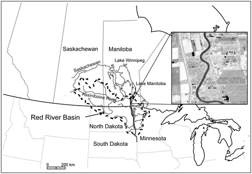
The Red River is situated in the central part of North America. It starts its flow path in Minnesota and flows towards the north. Forming the boundary between North Dakota and Minnesota, it enters Canada at Emerson, Manitoba. It continues its northward flow to Lake Winnipeg (Figure 2). Flooding is a common phenomenon in the Red River basin. Many floods took place in the twentieth century, such as in 1916, 1948, 1950, 1979, 1996, 1997 and 1999. A study area has been selected using the portion of the Red River flowing near the town of St. Adolphe to the south of Winnipeg with a length of about 5 km (Figure 2).

Figure 2. Location of the Red River Basin and study area for this study.

Data collection and GIS analysis

The first step in flood management is the identification of the flood-prone areas and the development of flood risk maps (Todini 1999). A risk map is developed in the present study using GIS to examine the topography of the study area, to classify it according to the surface level and to visualize the flooding conditions of the area. The topography of the study area is examined thoroughly by the generated DEM and TIN with a 5-m horizontal resolution and 15-cm vertical resolution.

A river flood is defined as the high flow of water that overtops either the natural or the artificial banks of a river (Smith 2002). For the purposes of the present study, five water surface levels are suggested, considering the flooded area based on 3D GIS mapping involving a 3D visualization of local infrastructures, and the expected consequent damages in each category. The risk levels associated with the water surface levels (WSL) can be characterized as follows:

1. Safe water surface level (WSL ≤ 232.25 m): this water surface level will not lead to any kind of risks associated with floods.

2. Slightly risky water surface level (232.25 m < WSL ≤ 233.19 m): only a few buildings adjacent to the river will be affected.

3. Highly risky water surface level (233.19 m < WSL ≤ 233.77 m): approximately 50% of the populated area will be flooded.

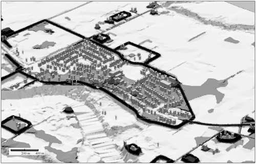
4. Extremely risky water surface level (233.77 m < WSL ≤ 234.28 m): this will cause the remaining 50% area to be flooded.

5. Totally flooded water surface level (WSL > 234.28 m): the whole area will be flooded for this type of flood.

The risk maps above are determined and presented using a 3D GIS approach involving spatial analysis as shown in Figures 3–6.

Figure 3. Risk map showing the predicted water level for the study area with the safe water surface level (< 232.25 m). (The white colour indicates the possibly flooded river area.)

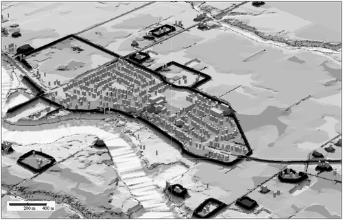
Figure 4. Risk map showing the predicted water level for the study area with the slightly risky condition (232.25–233.19 m).

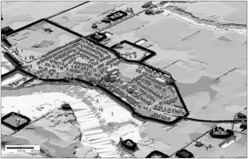
Figure 5. Risk map showing the predicted water level for the study area with the highly risky condition (233.19–233.77 m) indicating approximately 50% of the populated area is flooded.

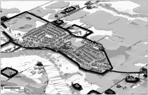
Figure 6. Risk map showing the predicted water level for the study area with the extremely risky condition (233.77–234.28 m) to cause the remaining 50% area to be flooded.

Hydraulic simulation

The hydraulic simulation is performed to obtain the relationship between the flow rate and the water surface level considering different flow rate scenarios. First, a conceptual model is developed using GIS data for the studied river valley. Figure 7 gives the conceptual model showing one set of simulation results for station 881.721. Five different flow rate scenarios, which are determined from the water surface levels denoting different flood risks, are used for input data to obtain the rating curves, which can be used along with the outputs of GIS analysis to determine the flow rates associated with different risk levels. Table 1 shows the simulation results of flow rates associated with different risk levels and water surface levels.

Figure 7. River reach for simulations and an example of predicted water surface levels for station 881.721.

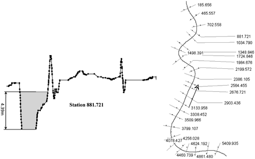
Table 1. Results for peak flow rates associated with different risk levels.

Risk level	Water surface level (m) WSL	Flow rate (m^3/s) FR
Safe	WSL ≤ 232.25	FR ≤ 1030.73
Slightly risky	232.25 < WSL ≤ 233.19	1030.73 < FR ≤ 1585.74
Highly risky	233.19 < WSL ≤ 233.77	1585.74 < FR ≤ 1981.90
Extremely risky	233.77 < WSL ≤ 234.28	1981.90 < FR ≤ 2389.94
Totally flooded	WSL > 234.28	FR > 2389.94

Statistical analysis

A multivariate regression technique is used to determine the relationship between the peak flow rate and the hydraulic and weather factors described previously. Equation (18) shows the regression model obtained using the historical data of the Red River from 1940 to 1999:(18)

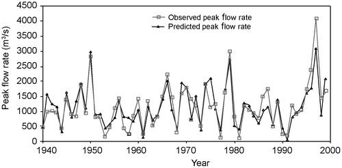
where PFR stands for the Peak Flow Rate [L³/T], API is the Antecedent Precipitation Index, MI is the Melt Index (mean degree-days/day), P denotes the total winter precipitation (L), which is the summation of WP (the water content of snowpack) and SP (the spring rain amount, L), and T stands for the timing factor (percent of worst south–north progression of melt snow and rain). Figure 8 shows a good agreement between the predicted and recorded values of PFR, with correlation coefficient r = 0.93, indicating the regression model is reasonably accurate. Nash-Sutcliffe efficiency (NSE) may also be used to indicate the model performance, with 1.0 indicating perfect model performance and 0 indicating that the model is performing only as well as the use of the mean target value as prediction (Nash and Sutcliffe 1970). The calculated NSE based on the predicted and observed peak flow rates (Figure 8) for this study is 0.80, indicating that the model performs well.

Figure 8. Comparison between the observed and predicted peak flow rates for 1940–1999.

The values of each factor that lead to different risk levels are determined by ordering the values of API, MI, P and T in descending order, and the corresponding flow rates are calculated using the developed regression formula. Thus, a risk criteria matrix is obtained as shown in Table 2, which shows the important input data set for the fuzzy flood risk model.

Table 2. Risk criteria for factors that affect the magnitude of the Red River flood.

Parameter	Safe	Slightly risky	Highly risky	Extremely risky	Totally flooded
Antecedent Precipitation Index (API)	2.20	2.37	2.71	2.90	2.95
Melt Index (MI)	6.46	7.43	9.00	10.27	11.08
Total Winter Precipitation (P) (cm)	9.30	10.21	12.70	13.67	14.94
Timing Factor (T) (%)	47.00	53.00	60.00	64.00	67.00

Fuzzy risk assessment model application

Two scenarios are used for the flood risk assessment based on the size of Red River flood for return periods of 25 years and 75 years. The historical data for the years 1940–1999 for the Red River region and the Log Pearson Type 3 distribution curve are used to determine the related hydrological information as input to the fuzzy-set risk model. Given the large amount of uncertainty associated with the system parameters, an interval analysis is incorporated into the fuzzy risk analysis model (Equations 8–14) to quantify the uncertainties associated with model inputs and outputs. In addition, a parameter-interval approach is applied to address the uncertainties associated with the four hydrological parameters (i.e., API, MI, P, T), and the lower and upper bounds of the intervals are determined considering safety or extreme values for the study region (Warkentin 1999). The determined interval values of the parameters that are used to assess the risk for the 25- and 75-year flood scenarios are given in Table 3.

Table 3. Parameters for two flood scenarios.

Parameter	25-year flood	75-year flood
Antecedent Precipitation Index (API)	2.20–2.24	2.86–2.89
Melt Index (MI)	6.8–7.3	11.7–13.1
Total Winter Precipitation (P) (cm)	10.72–11.58	17.45–20.80
Timing Factor (T) (%)	37–38	58–60

Two sets are then defined to apply the 3D GIS-FRA approach for flood risk assessment; U is the set of system factors and V is the set of risk levels:(19)

A fuzzy subset of U is introduced, A, which gives the membership grade for each parameter based on Equation (2). For the 25-year flood scenario, it is calculated as follows:(20)

A second fuzzy subset, which gives the membership value for each parameter versus different risk levels, is computed as follows based on Equations (5–14). Applying Equations (5) and (6) gives the following results:(21)

and(22)

from which the flood risk assessment result is given by:

For the lower bound of parameter values:

For the upper bound of parameter values:

Similar calculations were conducted for the 75-year flood scenario for the Red River region as follows:

For the lower bound of parameter values:

For the upper bound of parameter values:

Figures 9 and 10 show the results of the flood risk assessment approach. For the 25-year flood scenario, it is given that, since , the risk level is safe (Figure 9a); when more conservative inputs are used, the risk level can be , which gives a slightly risky situation (Figure 9b). Therefore, the risk level ranges from a safe to a slightly risky situation. Other values for and are helpful in providing additional information about the risk level for this scenario. For instance, as shown in Figure 9, = 0.79, indicates the occurrence of a slightly risky situation. On the other hand, , indicates that, while the risk level is slight, there is a greater likelihood of a safe situation than a highly risky one.

Figure 9. Results of risk assessment for 25-year flood scenario for: (a) lower bounds and (b) upper bounds.

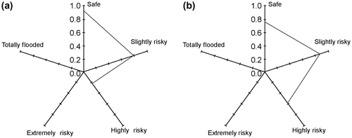
Figure 10. Results of risk assessment for 75-year flood scenario for: (a) lower bounds and (b) upper bounds.

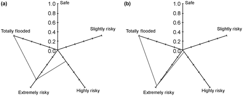
As for the 75-year flood scenario, since = = 1, the risk assessment indicates that the study area will be totally flooded. The risk results are deterministic, and the study area is totally flooded. However, as shown in Figure 10, = 0.79, indicating that there is the possibility of having an extremely risky situation in the lower bound; the possibility increases to 0.95 for the upper bound.

Referring to the GIS mapping of the study area, the risk assessment results show that the overall risk level ranges from a safe condition (Figure 3) to a slightly risky condition (Figure 4) for the 25-year flood scenario for the Red River region. Very limited impacts are expected on the town of St. Adolphe to the south of Winnipeg adjacent to the Red River if a 25-year flood occurs. Outputs from the 3D GIS-FRA for this scenario also indicate a possibility of having a highly risky situation (Figure 5) for the upper-bound extreme condition. Thus, the possibility of having up to 50% of the populated area flooded should be considered for emergency preparedness purposes. Similarly, for the 75-year scenario, the overall risk level is high which may cause the whole area of the town of St. Adolphe to be totally flooded. Additionally, the 3D GIS-FRA results also indicate the possibility of having an extremely risky situation (Figure 6), with 50–100% of the town area flooded for this scenario.

Conclusions

A 3D GIS-FRA approach was developed for flood risk assessment and impact management based on a fuzzy-set risk model, a river system simulation and 3D GIS mapping. Specifically, the risk model is designed to examine multiple critical hydrological factors contributing to the flood impacts. These impacts are subsequently integrated in a risk assessment with incorporation of a hydraulic simulation of river floods as well as a 3D GIS visualization of flood risks and impacts on the urban area. In addition, a parameter-interval analysis has been used to extend the 3D GIS-FRA to quantify the uncertainties associated with the key model parameters and the study system.

Application of 3D GIS-FRA to the Red River demonstrates that the developed approach can examine flood risks to the populated region systematically as well as the impacts on the local community in the flood plain area. It confirms that the developed fuzzy-set risk model can identify the integrated risk levels associated with possible flood scenarios, and within the GIS-FRA system framework the GIS-supported hydraulic analysis with DEM data provides a practical simulation of river flooding and a 3D visualization of quantified impacts on the urban region. Therefore, the developed GIS-FRA can be applied to other time series data and international cases to provide a comprehensive assessment of flood risk and impact.

Acknowledgements

This study was supported in part by the Natural Sciences and Engineering Research Council of Canada (NSERC). The authors are thankful to the reviewers for their helpful comments.

References

- Abdalla, R., C. Tao, H. Wu, and I. Maqsood. 2006. A GIS-supported 3D approach for flood risk assessment of the Qu’Appelle River, Southern Saskatchewan. International Journal of Risk Assessment and Management 6(4): 440–455.
- Ahmad, S. S., and S. P. Simonovic. 2011. A three-dimensional fuzzy methodology for flood risk analysis. Journal of Flood Risk Management 4(1): 53–74.
- Borri, D., G. Concilio, and E. Conte. 1998. A fuzzy approach for modelling knowledge in environmental systems evaluation. Computers, Environment and Urban Systems 22(3): 299–313.
- Brunner, G. 2001. HEC-RAS hydraulic reference manual. Davis, CA: US Army Corps of Engineers, Hydrologic Engineering Center.
- Burn, D. H. 1999. Perceptions of flood risk: A case study of the Red River flood of 1997. Water Resources Research 35 (11): 3451–3458.
- Chen, R. J. 2011. Impacts of natural disasters on regional economies: An overview. Tourism Analysis 16(3): 367–371.
- Chen, Z., G. H. Huang, and A. Chakma. 1998. Integrated environmental risk assessment for petroleum contaminated sites: A North America case study. Water Science and Technology 38: 129–136.
- Chuntian, C. 1999. Fuzzy optimal model for the flood control system of the upper and middle reaches of the Yangtze River. Hydrological Science 44: 573–582.
- Elmazoghi, H. G. 2013. Fuzzy algorithm for estimating average breach widths of embankment dams. Natural Hazards 68: 229–248.
- Environmental Systems Research Institute (ESRI). 2011. ArcGIS desktop: Release 10. Redlands, CA: ESRI.
- Haque, C. E. 2000. Risk Assessment, emergency preparedness and response to hazards: The case of the 1997 Red River Valley Flood, Canada. Natural Hazards 21: 225–245.
- Heijne, I. S. 1992. Fluvial flooding: Decision making in floodplain management. In Proceedings of the 3rd International Conference on Floods and Flood Management, edited by A. J. Saul, 119–129. Florence, Italy.
- Hoggan, D. H. 1989. Computer assisted floodplain hydrology and hydraulics. New York: McGraw-Hill.
- Jha, A., J. Lamond, R. Bloch, N. Bhattacharya, A. Lopez, N. Papachristodolou, and A. Bird. 2011. Five feet high and rising: Cities and flooding in the 21st century. Washington, DC: The World Bank.
- Kliskey, A. D., and A. E. Byrom. 2004. Development of a GIS-based methodology for quantifying predation risk in a spatial context. Transactions in GIS 8(1): 13–22.
- Kuzmin, V. B. 1981. A parametric approach to description of linguistic values of variables and hedges. Fuzzy Sets and Systems 6: 27–41.
- Lanza, L., and F. Siccardi. 1995. The role of GIS as a tool for the assessment of flood hazard at the regional scale. In Geographical information system in assessing natural hazards, edited by A. Carrara and F. Guzzetti, 199–217. Amsterdam: Springer.
- Leung, L. 1988. Spatial analysis and planning under imprecision. Amsterdam: Elsevier Science.
- Liu, L., J. Zhou, X. An, Y. Zhang, and L. Yang. 2010. Using fuzzy theory and information entropy for water quality assessment in Three Gorges Region, China. Expert Systems with Applications 37(3): 2517–2521.
- Nash, J. E., and J. V. Sutcliffe. 1970. River flow forecasting through conceptual models part I — A discussion of principles. Journal of Hydrology 10(3): 282–290.
- Pielke Jr, R. A. 1999. Nine fallacies of floods. Climatic Change 42(2): 413–438.
- Rahman, A., P. E. Weinmann, T. M. Hoang, and E. M. Laurenson. 2002. Monte Carlo simulation of flood frequency curves from rainfall. Journal of Hydrology 256: 196–210.
- Simonovic, S. 2005. A spatial Multi-Objective Decision-Making under uncertainty for water resources management. Journal of Hydroinformatics 7: 117–133.
- Singh, V. P., A. K. Rajagopal, and K. Singh. 1986. Derivation of some frequency distributions using the Principle of Maximum Entropy (POME). Advances in Water Resources 9(2): 91–106.
- Smith, K. 2002. Environmental hazards assessing risk and reducing disaster. London: Routledge.
- Todini, E. 1999. An operational decision support system for flood risk mapping, forecasting and management. Urban Water 1(2): 131–143.
- Warkentin, A. 1999. Red River at Winnipeg: Hydrometerologic parameter generated floods for design purposes. Winnipeg, MB: Manitoba Water Resources.
- Zimmermann, H. J. 2001. Fuzzy set theory and its applications. Norwell, MA: Kluwer Academic.