Evaluation of the Versatile Soil Moisture Budget model for a humid region in Atlantic Canada

Abstract

In this study, the performance of the Versatile Soil Moisture Budget (VSMB) model was evaluated to simulate soil water content (θ) for a study site near Truro, Nova Scotia, which is a humid region in Atlantic Canada. The risk associated with both surplus and deficit water in this region of Nova Scotia was also quantified. The average root mean squared error (RMSE), mean absolute error (MAE), coefficient of determination (R²), model efficiency (E) and index of agreement (d) of 3.63, 3.08, 0.9, 0.7 and 0.92, respectively, for a validation period (growing season of 2000) suggest that the model performed reasonably well in predicting θ. The results of analysis of simulated θ using the validated model for 1 April to 31 October over a period of 92 years (1910–2001) showed that the likelihood of having deficit [θ ≤ 50% available water (AW)] and severe deficit (θ ≤ 25% AW) events is higher in July and August and it is likely that such events will last longer than a single day. About 94% and 75% of the days in April and October, respectively, have trafficability problems [θ > 92.3% field capacity (FC)], while about 26.5% and 19.4% of the days in April and October, respectively, have crop surplus problems (θ > FC).

Abstract

Dans cette étude, l’exécution du modèle budget de l’ humidité du sol polyvalent (VSMB) a été évalué pour simuler la teneur en eau du sol (θ) pour un site près de Truro en Nouvelle-Écosse qui est une région humide dans le Canada atlantique. Le risque associé à la fois surplus et de l’eau du déficit dans les conditions dans cette region de la Nouvelle-Écosse a également été quantifiée. Signifie la racine moyenne erreur quadratique moyenne (RMSE), erreur absolue moyenne (MAE), le coefficient de détermination (R²), l’efficacité du modèle (E) et l’indice d’accord (d) de 3.63, 3.08, 0.9, 0.7 et 0.92, respectivement, pour une période de validation (saison 2000 en croissance), suggérant que le modèle fonctionne assez bien à prédire θ. Les résultats des analyses de simulation θ en utilisant le modèle validé pour la période du 1er avril à 31 octobre de 92 ans (1910 à 2001) ont montré que la probabilité d’avoir un événement déficit [θ ≤ 50% d’eau disponible (AW)] et une déficit sévère (θ ≤ 25% AW) est plus élevé en juillet et août et il est probable que l’événement durera plus longtemps que d’une seule journée. Environ 94 à 75% des jours en avril et octobre, respectivement, ont des problèmes de traficabilité [θ capacité au champ > 92.3% (FC)], alors qu’environ 26.5 et 19.4% des jours en avril et octobre, respectivement, ont des problèmes de surplus de récoltes (θ > FC).

Introduction

Soil moisture is an important hydrologic parameter that controls many land surface processes and is an integrated measure of several meteorological and physical properties (Narasimhan et al. 2005). From an agricultural perspective, soil water conditions are often less than ideal because conditions are frequently either too dry or too wet. Deficit soil water can severely minimize crop water uptake and thus yield. Surplus conditions can cause reductions in water and nutrient uptake due to poor aeration. Moreover, water surpluses limit crop production by delaying field operations involving planting, cultivation and harvesting (De Jong and Bootsma 1997). Soil moisture status is a good measure to assist in scheduling various agricultural operations including drought monitoring, yield forecasting and crop scouting. Hence, it can be a useful planning tool for the development of investment strategies (Heathman et al. 2003).

Difficulties with soil water measurement techniques associated with equipment as well as intensive labour requirements have made long-term soil water information difficult and expensive to compile (Chanasyk et al. 2004). These problems have supported the development of computer simulation models for simulating soil water content (θ). Numerous models have been developed, ranging in complexity from simple daily water budget models to more comprehensive generic models involving partial differential equations to calculate soil water flow (Elmaloglou and Malamos 2000). A water budget model, referred to as the Versatile Soil Moisture Budget (VSMB) model, was first proposed by Baier and Robertson (1966). It requires a limited amount of generally available input data (Chanasyk et al. 2004) and has been successfully used for several applications (Gallichand et al. 1991; Defaria et al. 1994; Baier and Robertson 1996; Qian et al. 2009; Hayashi et al. 2010).

The occurrence of surplus or deficit θ depends on conditions which are highly variable from year to year; therefore the probability of occurrence is the general method for reporting these types of data. Understanding the probability of deficit or surplus θ is essential for anticipating and mitigating possible damage (such as crop loss) and can be useful for probability-based management.

Nova Scotia is a humid region located in Atlantic Canada that experiences both surplus and deficit soil moisture conditions throughout the growing season (Nova Scotia Federation of Agriculture (NSFA) 2001). Therefore, a practical and accurate tool is needed for assisting in planning agricultural activities based on θ and the probability of surplus or deficit θ. However, there have been limited attempts to evaluate the performance of models to simulate θ for Nova Scotia’s conditions. Also, there has been no detailed information on the frequency or risk of surplus and deficit θ conditions. The present study evaluated the VSMB’s ability to estimate θ for a grass reference crop on a typical agricultural soil. The objectives of this study were (1) to calibrate the VSMB model for a site near Truro, Nova Scotia, and assess its ability to simulate θ and (2) to assess the risk of occurrence of water surplus or deficit conditions throughout the growing season using long-term model simulations for Truro, Nova Scotia.

Methods

Model description

The VSMB model is a soil water budget model that is continuous and deterministic in nature. It is a compromise between a completely empirical model, where no parameters involving physical processes are considered, and a mathematical model, in which only physical parameters are used (Baier et al. 1979). It is based on the premise that the water available for plant growth is gained by precipitation or irrigation, and lost through evapotranspiration and runoff as well as lateral and deep drainage (Baier et al. 2000; De Jong et al. 1992). The daily net loss or gain is added or subtracted from the water already present in the rooting zone. Water is withdrawn simultaneously, but at different rates, from different soil depths, depending on the potential evapotranspiration (PET), the stage of crop development, the water release characteristics of each soil layer and the available water (AW) (De Jong 1988). AW is defined as the difference between field capacity and permanent wilting point.

The advantage of this model is the limited amount of input data required while still providing sufficiently accurate output information (Boisvert et al. 1992). Inputs to the model include: soil physical data [saturation, field capacity (FC), permanent wilting point (PWP), initial soil moisture content (the budget starts at field capacity) and bulk density], soil factors (Z-curve), crop characteristic data [crop coefficient (K_c) and rooting depth], and daily meteorological information (maximum and minimum temperatures, precipitation and PET).

The PET is calculated within the model using Equations (1) and (2) (Baier et al. 2000): (1) (2)

where LE is daily latent evaporation (cm³), T_max is daily maximum temperature (°C), T_min is daily minimum temperature (°C) and Q₀ is computed theoretical radiation at the top of the atmosphere (gcal*cm⁻²) calculated from the latitude and day of year. The relationship between AW and the ratio of actual daily evapotranspiration (AET) to PET depends on the physical characteristics of the soil as well as the stage of crop growth. The VSMB model makes use of standard empirical curves (Z-curves) for this purpose (De Jong 1988). The Z-curves are soil moisture drying curves, which reflect soil characteristics in relation to water demands by the crop. They are controlled by coefficients (MZ, NZ, RZ and HZ), which are defined independently of the AW (Dyer and Baier 1979). These produce curve shapes of linear (MZ = 1; NZ = 0), upward concave (MZ = 1; NZ = 1; HZ = 0 to 1) or convex (MZ = 1; NZ = 1; HZ = 1 or greater). Two Z-curves may be entered for each zone: one for fallow conditions and one for cropped conditions (Baier et al. 2000). Crop coefficients should also be determined to approximate changes in root densities over time and soil depth, and can be interpreted as an index for root densities (Dyer and Dwyer 1982). To take into account the structure and texture of the soil, root development and transpiration ability of plants, the plant cycle should be divided into periods so that each period starts with a set of crop coefficients (K_c) (Belmans et al. 1979). Therefore, K_c value should be provided for each zone during each growth stage.

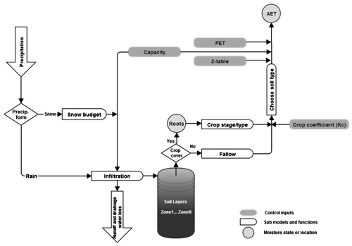
In the VSMB, the water that is allowed to infiltrate is limited to the lesser of either the variable defined as input data or, by default, the amount of water required to bring all soil zones (Zone1 ….Zone N) of the infiltrated drainage layer to saturation. The surface water or the water in excess in each zone of a drainage layer is allowed to leave the surface or a drainage layer (Baier et al. 2000). A schematic summary of the soil-root-atmosphere pathways of water in the VSMB is shown in Figure 1 (adapted from Baier et al. 1979). A complete description of the model is available in Baier et al. (2000).

Figure 1. Soil-root-atmosphere pathways of water in the Versatile Soil Moisture Budget model (VSMB; adapted from Baier et al. 1979). N is the number of soil zones, which is flexible in this model. The deepest zone usually corresponds to the maximum rooting depth. The snow budget function was not used in this study.

Site description and measurements

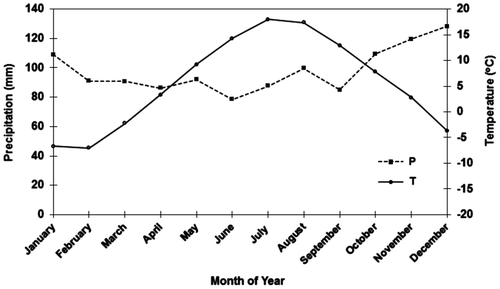
The study was conducted adjacent to the Environment Canada climate station (45°22′N, 63°16′W) on the campus of the Nova Scotia Agriculture College (now Faculty of Agriculture, Dalhousie University) in Truro, Nova Scotia. In the study area, the mean annual temperature and precipitation are 5.5°C and 1176 mm, respectively. Figure 2 shows average monthly temperature (T) and precipitation (P) for the experimental site.

Figure 2. Average monthly (for the 30-year period) precipitation (P) and temperature (T) for the experimental site.

The θ and daily meteorological data were obtained for three consecutive growing seasons (1998 to 2000) at the experimental site. The site was covered with a mixture of grass and clover. The grasses were creeping red fescue (Festuca rubra) with some bluegrass. Grass is often used as a reference crop for soil moisture modeling (Omer et al. 1988) as done in this study. In the model, the growth stages were considered as planting to emergence (after 75 degree days are accumulated), emergence to heading (after 650 degree days are accumulated), heading to jointing (after 1350 degree days are accumulated), jointing to soft dough (after 1500 degree days are accumulated) and soft dough to ripening (end of run) (Gregoire et al. 2000).

Soil cores were collected and analyzed to determine the soil information required for input to the model. For this study, three soil layers were used (0 to 30, 30 to 50 and 50 to 100 cm soil depth) which correspond to the A, B and C horizons. These soil layers also correspond to zones 1 to 3 in the VSMB model. Ten undisturbed cores were collected for each of the three soil horizons, resulting in a total of 30 soil cores. Soil bulk density, saturated hydraulic conductivity and soil water retention characteristics were determined using standard laboratory procedures on undisturbed soil cores (Sheldrick 1984). The soil analysis determined that the predominant soil type at the site is Pugwash 82 (Agriculture and Agri-Food Canada 2013), a typical agricultural soil for Nova Scotia. It is well drained and has greater than 80 cm of friable, coarse loamy soil over firm, coarse loamy lower soil material (Webb et al. 1991). Several soil characteristics for this site are listed in Table 1.

Table 1. Soil parameters at the experimental site for three soil depths.

Soil parameters	Depth (cm)
	0–30	30–50	50–100
Clay (%)	10.0	11.1	11.9
Silt (%)	31.2	27.5	23.2
Sand (%)	58.8	61.5	64.9
Texture	Sandy loam	Sandy loam	Sandy loam
Bulk density (g cm^−3)	1.23	1.30	1.46
Field Capacity (% volume)	24.7	20.6	16.4
Permanent wilting point (% volume)	6.0	11.0	7.9
Organic matter (%)	4.2	2.1	1.6
pH	5.9	5.5	5.3

The θ measurements collected at the site were for the 0 to 30 cm soil layer. The measurements were made using Campbell Scientific CS615 TDR soil moisture probes and recorded using a CR10 datalogger. The pairs of stainless steel rods, 30 cm long and 3.2 mm in diameter, were inserted vertically into the soil and were calibrated after installation. They were installed and arranged randomly in batches (3 to 9 per batch), and recorded θ values were averaged. The θ measurement was made daily during the study period without replication.

Model calibration and validation

Calibration is the process where the model’s input parameters are changed to obtain the optimal agreement between the predicted and observed variables (Singh et al. 2006). Calibration of the VSMB model (version 2000) was performed with field-measured θ values collected during the 1998 and 1999 growing seasons (15 May to 30 September in 1998 and 30 April to 12 October in 1999). The model was calibrated for the upper horizon of the soil (0 to 30 cm) since this is the layer of concern for most crops with respect to surplus and deficit θ. Meteorological input data included daily maximum and minimum temperatures (°C) and precipitation (mm), which were collected at the Environment Canada climate station directly adjacent to the location where θ was measured. To select the parameters for the calibration process, the input parameters were changed (one input parameter at a time) and then the change in the simulated θ was observed. Once the simulated soil moisture changes and trends were observed and the parameters for calibration selected, the calibration process began. During the calibration process, adjustments were made to several model inputs including: FC, PWP, K_c and Z curve to improve model performance. The calibration parameter values were then increased and decreased, and at each step of the calibration process the change in the soil moisture values was observed and the accuracy of the simulations was estimated by the computation of five indices (Legates and McCabe 1999). Final best calibration parameters were selected from the simulation with the greatest number of “best” values for all five indices. These indices include:

The root mean squared error (RMSE): (3)

where P_i is the model simulated value (daily), O_i is the observed value (daily), n is the number of values and i is the index for the number of values.

The mean absolute error (MAE):(4)

The coefficient of determination (R²): (5)

where is the mean of observed values (O_i) and is the mean of simulated values (P_i).

The modeling efficiency (E):(6)

The index of agreement (d):(7)

E evaluates the error relative to the natural variation of the observed values (Singh et al. 2006) and d measures the agreement between the simulated and observed θ (Willmott 1982). In the calibration process, attempts were made to minimize RMSE and MAE and obtain R², d and E closest to unity by adjusting the selected input parameters (Legates and McCabe 1999).

The calibrated model parameters were then used to validate the model using data collected during the 2000 growing season (25 April to 4 October). Soil, crop and field model inputs were identical to those utilized in the calibration simulation. The model was also statistically evaluated in the same manner as for the calibration years.

Long-term simulation of θ

The validated VSMB model was then used to simulate daily θ for the 0 to 30 cm soil layer for 1 April to 31 October over a period of 92 years (1910 to 2001) using historical meteorological data for Truro, Nova Scotia. The long-term simulations were then analyzed to determine the frequency and risk of deficit and surplus θ conditions. In this study, deficit θ was considered as daily θ < 50% AW at which the growth of most plants is limited and yield is reduced (De Jong et al. 1991). Severe deficit θ was defined as lower than 25% AW, at which severe crop damage can be expected (Meyer and Green 1981). Surplus θ is defined either based on surplus θ for the plant or surplus θ for field machinery. Surplus θ with respect to the plant growth can be considered as θ > FC (Lake and Broughton 1968), while surplus θ for machinery occurs at θ < FC (Selirio and Brown 1972). For this investigation, θ > 92.3% FC was considered as the trafficability surplus θ. This value is the average of the θ values suggested by Selirio and Brown (1972), Baier (1973) and Sheldrick (1984). After determination of deficit and surplus θ, soil water indices (SWI) were determined for each simulation year. The soil water indices were determined using the daily θ from 1 April to 31 October of each simulation year which indicates whether or not a year is a surplus or deficit. The index value for a year was obtained by calculating the total number of days at a particular %AW or %FC.

The frequency of occurrence of various θ values and SWI are just two ways of evaluating the possibility of deficit and surplus θ conditions. In order to accurately study the simulated conditions, the probability distribution was examined, which is a more powerful and useful analytical research tool (Dyer and De Jager 1986; Baier and Robertson 1996). The number of consecutive days of a specific occurrence is important because the longer the duration of a deficit or surplus θ, the greater the damage to the plant and reduction in yield. Stewart and Neilsen (1990) found that short daily stress periods of deficit conditions are less damaging than infrequent periods that last for several days. For this study, the number of consecutive days of occurrence of either deficit or surplus θ was fitted to a probability distribution using the BestFit software for Windows version 2.0 (Palisade Corporation 1996). Probability distributions for the length of occurrence of soil moistures greater or less than specified values (25% AW, 50% AW, 92.3% FC and FC) were generated.

Results

Model calibration

Comparison of the observed and simulated data shows some agreement during the calibration years (Figure 3), but systematic offset is present. This could be due to some model limitations. In this model, duration and intensity of precipitation (within a day) are not taken into account. Also, variable states of the soil such as soil water tension or hydraulic conductivity and root densities are not considered in the physical terms (Baier et al. 2000).

Figure 3. Measured (•) and simulated (—) volumetric soil moisture for 0–30 cm soil depth during calibration years (a) 1998 and (b) 1999.

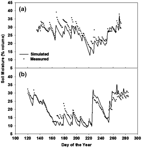
The statistical measures of the calibration results are shown in Table 2. The RMSE and MAE, which are among the best overall measures of model performance (Willmott 1982), had an average of 3.08 and 2.50, respectively (Table 2). The R² was 0.75 (in 1998) and 0.89 (in 1999), which suggests that the model performance was reasonable in predicting θ during the calibration years (Table 2). The average values of E and d during the calibration were 0.63 and 0.92, respectively, showing a reasonable agreement between simulated and observed θ (Table 2). Final best calibration parameters are presented in Table 3.

Table 2. Statistical performance of the VSMB model to predict soil moisture during the calibration years (1998, 1999) and validation year (2000). RMSE: Root mean squared error; MAE: Mean absolute error; R²: coefficient of determination; E: Model efficiency; d: Index of agreement.

Year	RMSE (% volume)	MAE (% volume)	R^2	E	d
1998	3.33	2.73	0.75	0.47	0.87
1999	2.82	2.27	0.89	0.79	0.96
Mean (1998 and 1999)	3.08	2.50	0.82	0.63	0.92
2000	3.63	3.08	0.90	0.70	0.92

Table 3. The final best calibration parameters.

Model input	Parameter
Field capacity (% volume)	24.7
Permanent wilting point (% volume)	6.0
Z-curve values (MZ, NZ, RZ, HZ)	MZ = 1, NZ = 1, RZ = 0.23, HZ = 1.62
Crop coefficients^1	Growth stage 1: 0.54; Growth stage 2: 0.58; Growth stage 3: 0.64; Growth stage 4: 0.72; Growth stage 5: 0.72

¹ Crop coefficients: growth stages refer to planting to emergence (after 75 degree days are accumulated), emergence to heading (after 650 degree days are accumulated), heading to jointing (after 1350 degree days are accumulated), jointing to soft dough (after 1500 degree days are accumulated) and soft dough to ripening (end of run), respectively.

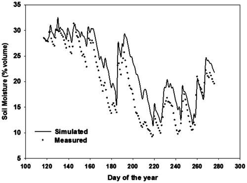
Comparison of measured and simulated θ values for the validation year (2000) show that the magnitude and trend in the simulated θ values follow the measured data, but again with some systematic offset (Figure 4). The RMSE and MAE of the model were 3.63 and 3.08, respectively (Table 2). The R² indicates that the model explained 90% of the variability in the observed θ measurements. The E of 0.70 suggests that the model produced a reasonable agreement with observed θ values. The d was close to unity (0.92), suggesting that the model performed reasonably well in predicting θ (Table 2).

Figure 4. Measured (•) and simulated (—) volumetric soil moisture for 0–30 cm soil depth during validation year (2000).

Frequency of occurrence

The θ simulated for 92 years spanning 1 April to 31 October (1910 to 2001) was examined for the frequency of deficit (θ ≤ 50% AW), severe deficit (θ ≤ 25% AW) and surplus (θ > 92.3% FC for trafficability and θ > FC for plants) soil water conditions. The frequency of occurrence was also determined on a monthly basis to provide a more detailed look at when specific θ values occurred during the investigative period. Table 4 summarizes the frequency of occurrence based on the number of days of deficit or surplus θ for the entire growing season period, analyzed on a monthly basis. It shows, as expected, that deficit and severe deficit θ conditions are dominant during July and August. Almost 50% of the days in August are < 50% AW, suggesting that some reduction in crop yield can be expected (Table 4). This also happens during about 40% of the days in July. Surplus θ is a major concern during April, May, September and October, revealing that some trafficability problems may occur during these months (Table 4). Thus, the machinery would not be able to work at harvesting of some crops.

Table 4. Probability (%) of severe deficit θ (θ ≤ 25% AW), deficit θ (θ ≤ 50% AW), surplus θ for machinery (θ > 92.3% FC) and surplus θ for plants (θ > FC) based on the number of days of occurrence for the growing season analyzed and on a monthly basis. θ: moisture content; FC: field capacity.

Occurrence	Growing season	Apr.	May	June	July	Aug.	Sept.	Oct.
Severe deficit θ	8.8	0	0.4	4.7	17.2	24.9	11.7	2.2
Deficit θ	20.2	0	1.4	18.4	40.1	46.5	28.8	5.5
Surplus θ for trafficability	45.6	94.20	58.7	26.8	15.6	15.3	34.7	74.6
Surplus θ for plants	9.4	26.50	9.6	2.7	1.6	1.8	4.0	19.4

Soil Water Index (SWI)

The simulation results obtained based on the SWI which display a severe deficit, deficit and surplus (for machinery and plants) years are shown in Figure 5. It shows that deficit and severe deficit θ have been quite variable over the growing seasons from 1910 through 2001. Specifically, it shows that 1960 experienced an 86-day severe deficit, followed by 1975 at 69 and 2001 at 61, while 1960, at 140, experienced the highest number of deficit days, followed by 1921 at 115 and 1918 at 102. Moreover, the graph reveals that 21 out of the 92 years (about 23%), or about 1 out of every 4 years, did not experience a severe deficit day. In other words, 3 out of every 4 years experienced at least 1 severe deficit day (Figure 5). The median of 10 indicates that 1 out of every 2 years will experience severe deficit θ for more than 10 days during a growing season (Figure 5). The results also show that 5 out of the 92 years (about 5%) never experienced a deficit day (Figure 5). The median of 37 days indicates that 1 out of every 2 years will experience deficit θ for more than 37 in a season (Figure 5). These results reveal that installation of an irrigation system may avoid yield reductions. In this regard, a cost-benefit analysis must be carefully considered by policy-makers.

Figure 5. Soil water index (SWI) for (a) severe deficit θ (θ ≤ 25% AW), (b) deficit θ (θ ≤ 50% AW), (c) surplus θ for machinery (θ > 92.3% FC), (d) and surplus θ for plants (θ > FC) for the period of 1 April to 31 October of each simulation year. θ: moisture content; AW: available water; FC: field capacity.

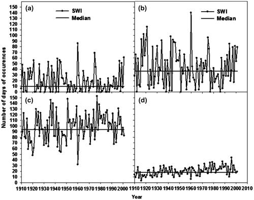
The results also show that surplus soil moistures were quite variable over the 92 years examined (Figure 5). It specifically shows that 1977, at 153, experienced the highest number of days with surplus θ for machinery, followed by 1951 at 148, 1936 at 146 and 1938 at 140 days. This suggests that, on average, surplus θ for trafficability may happen for 94 days of the-214 day season, or 44% of the time. These soil moisture levels could actually be beneficial to plant growth, unless they occur solely at planting and harvesting. However, as shown in Table 4, most of the days that have surplus θ for trafficability are at planting and harvesting times. This suggests that installation of drainage systems in this region can help farmers to work in their fields more efficiently. As shown in Figure 5, on average, surplus θ for plants will occur for 18 days of the 214-day season, or 8% of the time. However, unless these moisture levels occur after the crops have been planted and for many days at one time they will not cause yield reduction. According to Table 4, surplus θ for crop primarily occurs in April and October and frequently occurs in May and September. Therefore, it is clear that crop damage is very unlikely in June, July and August in this region, due to surplus soil moisture. The most common months for possible crop damage due to surplus soil moisture would, however, be April and October. Therefore, early planting or late harvesting could severely damage the crop on average approximately 23% of the time or 1 out of every 5 years (Table 4).

Probability distribution

Different probability distributions were tested for the data and the appropriate distribution function was identified based on the Chi-squared (Hines et al. 2003), Kolmogorov-Smirnov (Law and Kelton 2000) and Anderson-Darling (Anderson 1954) values. No identifiable distribution for the soil moisture greater than FC and 92.3% FC were found and these data did not follow a known distribution pattern. However, the best-fit distribution for θ < 25 and 50% AW was found to be lognormal (μ: the population mean, ϭ: the population standard deviation). The probability distribution and the estimated values of μ and ϭ are presented in Figure 6.

Figure 6. Number of events for consecutive days occurrences and the corresponding frequency distribution for (a) deficit θ (θ ≤ 50% AW) and (b) severe deficit θ (θ ≤ 25% AW). θ: moisture content; AW: available water.

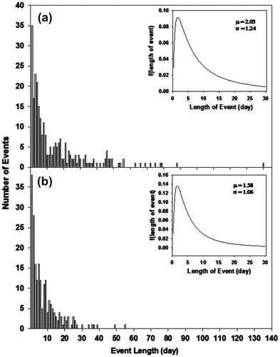
The number of events for consecutive days with severe deficit and deficit θ during the study period (1 April to 31 October of 1910 to 2001) are shown in Figure 6. There are 68 events for deficit θ that lasted 20 days or longer. If it is assumed that 1 event occurs per year, in about 74% of the years (68 events in 92 years) soil moistures will be < 50% AW for a period of 20 consecutive days or longer. This could have serious consequences for crops. The four longest consecutive days with deficit θ were found to be 78, 79, 88 and 140 days (Figure 6) which happened during 1997, 2001, 1945 and 1960, respectively (data not shown). The severe province-wide drought in Nova Scotia reported in 1997 and 2001 (NSFA 2001) confirms these simulation results.

Table 5 shows the probability of occurrence of an event from the distribution which was created using only θ values < 50 or 25% AW. The probability of occurrence of an event for an entire growing season period (1 April to 31 October) or specific period (July and August) was obtained by combining data in Table 4 with the probability of the length of an event. This shows that, if θ is < 50% AW, 9% of the time that event will last for 2 days (Table 5). The probability of having a 2-day-long event during the period is 1.8% and the probability of having an event longer than 2 days is 17.4%, for the entire growing season. However, the probability of a 2-day event in July and August is 3.9% and the probability of longer event is 37.2%. Therefore, the probability is low that any given day during the period will be a day with deficit θ; however, for July and August the probability is quite high (43.3%). It has also been shown in the SWI results that only 5 out of 92 years experienced no deficit days. These findings suggest that the probability of θ being < 50% AW sometime in July and August is very high.

Table 5. Probability of consecutive days of occurrence (%) for deficit θ (θ ≤ 50% AW) and severe deficit θ (θ ≤ 25% AW) from distribution, for entire growing season period (April 1 to October 31) and July and Aug. θ: moisture content; AW: available water.

Event length (days)	Probability from distribution (%)			Probability for entire growing season period (%)			Probability for July and Aug. (%)
	Deficit θ	Severe deficit θ		Deficit θ	Severe deficit θ		Deficit θ	Severe deficit θ
1	5.1	6.8		1.0	0.6		2.2	1.4
2	9.0	13.4		1.8	1.2		3.9	2.8
3	8.6	12.3		1.7	1.1		3.7	2.6
4	7.6	10.3		1.5	0.9		3.3	2.2
5	6.5	8.3		1.3	0.7		2.8	1.8
6	5.7	6.8		1.1	0.6		2.5	1.4
7	4.9	5.6		1.0	0.5		2.1	1.2
8	4.3	4.6		0.9	0.4		1.9	1.0
9	3.8	3.9		0.8	0.3		1.6	0.8
10	3.3	3.3		0.7	0.3		1.4	0.7
11–20	19.4	15.7		3.9	1.4		8.4	3.3

Figure 6 also depicts 22 events with severe deficit θ lasting 20 days or longer. This is one-third of the number of deficit θ events that occurred during the same 92-year period. This result reveals that drier the conditions the less often it occurs. The results also demonstrate that 22 times in 92 years that a severe deficit θ occurs, it lasts for an extended period of time (at least 20 days). If it is assumed that one event happens per year, this indicates that about 24% (22 times in 92 years) of years (or 1 in every 4 years) will experience severe deficit soil moistures for a period of 20 consecutive days or longer. This could have serious consequences for crops. The three longest events for severe deficit θ were found to be 55 days in 1997, 49 days in 2001 and 39 days in 1911. It is known that severe crop damage occurred in 1997 and 2001, as was generally reported (NSFA, 2001).

Table 5 shows that 13.4% of the time that θ is < 25% AW, the event will last for 2 days. On an investigative-period basis, the probability of having a 1-day-long event is 0.6% and the probability of having an event longer than 1 day is 8.2%, for the entire growing season period.

The probability that a 1-day severe-deficit θ event will occur in July and August is 1.4%, while the probability of such an event lasting longer than 1 day is 19.7%. Therefore, the probability is low that any given day will be a day with severe deficit θ. However, this probability rises when July and August are considered. The SWI results show that only 21 years out of 92 (about 23%) never experienced severe deficit θ (Figure 5) and that they were not rare occurrences. The recommended irrigation threshold is 50% AW (Hanson et al. 2000) so many high-valued crops should never even reach this point (θ ≤ 25% AW) if quality and yield are to be maintained. Therefore, a cost analysis for higher-valued crops to avoid this situation is recommended.

Conclusion

The VSMB model was able to predict soil moisture with some accuracy during three growing seasons at a study site near Truro, Nova Scotia. The model was calibrated and validated for a grass reference crop. The calibration was performed using field-measured θ values collected during the 1998 and 1999 growing seasons. The model was then validated using the data collected during the 2000 growing season. The simulations confirmed a reasonable agreement between measured and predicted values, but with a persistent offset that might be explained by limitations related to duration and intensity of precipitation (within a day) which are not taken into account in VSMB. Overall, the results suggest that the VSMB model has potential for future use in Nova Scotia.

Understanding the frequency of occurrence of surplus and deficit θ is essential for agricultural planning. Long-term θ simulation using the VSMB model allowed the frequency of surplus and deficit θ to be assessed (for the period of 1 April to 31 October). The results suggest that machinery-surplus soil moisture is a major problem in April and October, with approximately 94% and 75% of the days in these months having θ > 92.3% FC, respectively. Crop surplus θ is also a problem in April and October, with approximately 26.5% and 19.4% of the days in that month having θ > FC, respectively. Approximately 40% and 45% of the days in July and August, respectively, had a deficit θ problem. On average, 3 in 4 years will experience deficit θ conditions for a period of 20 consecutive days or longer. Also, 3 out of every 4 years will experience at least 1 day with severe deficit θ. On average, 1 year in 2 and 1 year in 4 will experience severe deficit θ for a period of 10 consecutive days and 20 consecutive days (or longer), respectively.

References

- Agriculture and Agri-Food Canada. 2013. Profiles for Nova Scotia soil code PG82~~(Pugwash). http://sis.agr.gc.ca/cansis/soils/ns/PGW/82~~~/profiles.html (accessed January, 2014).
- Anderson, T. W. 1954. A test of goodness of fit. Journal of the American Statistical Association 49: 765-769.
- Baier, W. 1973. Estimation of field workdays in Canada from the versatile soil moisture budget. Canadian Agricultural Engineering 15: 84-87.
- Baier, W., J. B. Boisvert, and J. A. Dyer. 2000. The versatile soil moisture budget reference manual. Ottawa: Agriculture and Agri-Food Canada, Eastern Cereal and Oilseed Research Centre.
- Baier, W., J. A. Dyer, and W. R. Sharp. 1979. The versatile soil moisture budget. Bulletin 87, LRRC, Research Branch. Ottawa: Agriculture Canada.
- Baier, W., and G. W. Robertson. 1966. A new versatile soil moisture budget (VSMB). Canadian Journal of Plant Science 45: 299-315.
- Baier, W., and G. W. Robertson. 1996. Soil moisture modelling: Conception and evolution of the VSMB. Canadian Journal of Soil Science 76: 251-261.
- Belmans, C., J. Feyen, and D. Hillel. 1979. An attempt at experimental validation of macroscopic-scale models of soil moisture extraction by roots. Soil Science 127: 174-186.
- Boisvert, J. B., J. A. Dyer, R. Lagace, and P. A. Dube. 1992. Estimating water-table fluctuations with a daily weather-based water budget approach. Canadian Agricultural Engineering 34: 115-124.
- Chanasyk, D. S., E. Mapfumo, W. D. Willms, and M. A. Naeth. 2004. Quantification and simulation of soil water on grazed fescue watersheds. Journal of Range Management 57: 169-177.
- Defaria, R. T., C. A. Madramootoo, J. Boisvert, and S.O. Prasher. 1994. Comparison of the versatile soil moisture budget and SWACROP models for a wheat crop in Brazil. Canadian Agricultural Engineering 36: 57-68.
- De Jong, R. 1988. Comparison of two soil-water models under semi-arid growing conditions. Canadian Journal of Soil Science 68: 17-28.
- De Jong, R., and A. Bootsma. 1997. Estimates of water deficits and surpluses during the growing season in Ontario using the SWATRE model. Canadian Journal of Soil Science 77: 285-294.
- De Jong, R., A. Bootsma, J. Dumanski, and K. Samuel. 1991. Variability of soil water deficiencies for perennial forages in the Canadian prairie region. Agricultural Water Management 20: 87-100.
- De Jong, R., A. Bootsma, J. Dumanski, and K. Samuel. 1992. Characterizing the soil water regime of the Canadian prairies. Ottawa: Research Branch, Agriculture Canada.
- Dyer, J. A., and W. Baier. 1979. Weather-based estimation of field workdays in fall. Canadian Agricultural Engineering 21: 119-122.
- Dyer, J. A., and J. A. De Jager. 1986. Interpolation of threshold soil moisture levels from soil moisture frequency distributions. Water International 11: 127-132.
- Dyer, J. A., and L. M. Dwyer. 1982. Root extraction coefficients for soil moisture budgeting derived from measured root densities. Canadian Agricultural Engineering 24: 81-86.
- Elmaloglou, S., and N. Malamos. 2000. Simulation of soil moisture content of a prairie field with SWAP93. Agricultural Water Management 43: 139-149.
- Gallichand, J., R. S. Broughton, J. Boisvert, and P. Rochette. 1991. Simulation of irrigation requirements for major crops in south western Quebec. Canadian Agricultural Engineering 33: 1-9.
- Gregoire, T., G. Endres, and R. Zollinger. 2000. Identifying leaf stages in small grain. Fargo, ND: NDSU Extension Services, North Dakota State University of Agriculture and Applied Science and US Department of Agriculture Cooperating.
- Hanson, B. R., S. Orloff, and D. Peters. 2000. Monitoring soil moisture helps refine irrigation management. California Agriculture 54(3): 38-42.
- Hayashi, M., J. F. Jackson, and L. Xu. 2010. Application of the versatile soil moisture budget model to estimate evaporation from prairie grassland. Canadian Water Resources Journal 35(2): 187-208.
- Heathman, G. C., P. J. Starks, L. R. Ahuja, and T. J. Jackson. 2003. Assimilation of surface soil moisture to estimate profile soil water content. Journal of Hydrology 279: 1-17.
- Hines, W. W., D. C. Montgomery, D. M. Goldsman, and C. M. Borror. 2003. Probability and statistics in engineering. New York: John Wiley & Sons Inc.
- Lake, E. B., and R. S. Broughton. 1968. Soil moisture deficits and surpluses in south western Quebec. Hamilton, ON: Canadian Society of Agricultural Engineering.
- Law, A. L., and W. D. Kelton. 2000. Simulation modeling and analysis. Boston, MA: McGraw-Hill.
- Legates, D. R., and G. J. McCabe. 1999. Evaluating the use of ‘goodness-of-fit’ measures in hydrologic and hydroclimatic model validation. Water Resources Research 35: 233-241.
- Meyer, W. S., and G. C. Green. 1981. Plant indicators of wheat and soybean crop water stress. Irrigation Science 2: 167-176.
- Narasimhan, B., R. Srinivasan, J. G. Arnold, and M. Di Luzio. 2005. Estimation of long-term soil moisture using a distributed parameter hydrologic model and verification using remotely sensed data. Transactions of the ASAE 48: 1101-1113.
- Nova Scotia Federation of Agriculture (NSFA). 2001. Compendium of information regarding drought. Truro, NS: Nova Scotia Federation of Agriculture.
- Omer, M. A., K. E. Saxton, and D. L. Bassett. 1988. Optimum sorghum planting dates in western Sudan by simulated water budgets. Agricultural Water Management 13: 33-48.
- Palisade Corporation. 1996. BestFit for Windows. Newfield, NY: Palisade Corporation.
- Qian, B. D., R. De Jong, R. Warren, A. Chipanshi, and H. Hill. 2009. Statistical spring wheat yield forecasting for the Canadian prairie provinces. Agricultural and Forest Meteorology 149: 1022-1031.
- Selirio, L. S., and D. M. Brown. 1972. Estimation of spring workdays from climatological records. Canadian Agricultural Engineering 14: 79-81.
- Sheldrick, B. H. 1984. Analytical methods manual. LRRI Contribution No. 84-30. Ottawa: Land Resource Research Institute.
- Singh, R., M. J. Helmers, and Z. M. Qi. 2006. Calibration and validation of DRAINMOD to design subsurface drainage systems for Iowa’s tile landscapes. Agricultural Water Management 85: 221-232.
- Stewart, B. A., and D. R. Nielsen. 1990. Irrigation of agricultural crops, No. 30. Madison, WI: American Society of Agronomy.
- Webb, K. T., R. L. Thompson, B. J. Beke, and J. L. Nowland. 1991. Soils of the colchester county, Nova Scotia. Ottawa: Agriculture Canada.
- Willmott, C. J. 1982. Some comments on the evaluation of model performance. Bulletin of the American Meteorological Society 63: 1309-1313.