Assessing the impact of climate change on the frequency of floods in the Red River basin

Abstract

The impact of climate change on the frequency distribution of spring floods in the Red River basin is investigated. Several major floods in the last couple of decades have caused major damages and inconvenience to people living in the Red River flood plain south of Winnipeg, and have raised the question of whether climate change is at least partly responsible for what appears to be more frequent occurrences of high spring runoff. To investigate whether this is the case, a regression model is used to associate spring peak flow at the US–Canada border with predictor variables that include antecedent precipitation in the previous fall (used as a proxy for soil moisture at freeze-up), winter snow accumulation and spring precipitation. Data from the Coupled Model Intercomparison Project – Phase 5 (CMIP5) are used to derive information about possible changes to the predictor variables in the future, and this information is then used to derive flood distributions for future climate conditions. While mean monthly precipitation during the winter months is expected to increase, winters are expected to be shorter in warmer climates and evaporation losses are expected to be higher, resulting in a net reduction in average snow pack accumulations. On the other hand, precipitation during the active snowmelt period is expected to increase. The average of future flood distributions obtained from an ensemble of 16 climate models is close to the distribution fitted to observed data, but there is considerable uncertainty surrounding the average, highlighting the difficulty in assessing changes in the frequency of extreme events.

Dans cet article, nous essayons de déterminer l'effet des changements climatiques sur la fréquence des crues de la rivière Rouge. Dans les quelques dernières décennies, plusieurs inondations graves ont causé des dommages importants et perturbé la vie des personnes qui habitent à proximité de la rivière, au sud de la ville de Winnipeg, et soulevé la question à savoir si les changements climatiques contribuent à ce qui semble être une occurrence plus fréquente d’eaux de ruissellement élevées. Afin de répondre à cette question, nous utilisons un modèle de régression pour estimer le débit de pointe au printemps à la frontière entre le Canada et les États-Unis, en fonction des variables explicatives qui incluent la précipitation de l'automne précédent (qui serve à calculer approximativement l’humidité du sol au gel), ainsi que les précipitations hivernales et printanières. Le modèle de régression est estimé à partir de données historiques. Les données du Projet d’intercomparaison de modèles climatiques (CMIP5) sont utilisées pour obtenir de l’information sur des changements éventuels possibles des variables explicatives du modèle de régression, information qui servira par la suite à estimer la distribution statistique des crues selon les conditions climatiques futures. Les modèles climatiques indiquent que dans les climats plus chauds, les précipitations hivernales augmenteront, que les hivers seront plus courts et que les pertes en évaporation hivernale seront plus élevées, ce qui entrainera une réduction nette de la moyenne des accumulations de neige. On doit s'attendre par contre à une augmentation des précipitations pendant la période active de fonte des neiges. En ce qui concerne la distribution des crues printanières, la courbe moyenne d'un ensemble de 16 modèles climatiques globaux est comparable à celle estimée à partir des données historiques. Cependant, la variation des divers membres de l'ensemble autour de la moyenne est considérable, ce qui souligne la difficulté de déterminer les changements climatiques dans la fréquence des valeurs extrêmes.

Introduction

The Canadian Prairie provinces (Alberta, Saskatchewan, Manitoba) have experienced a number of severe flood events in recent years. Notable examples include the 1997 Red River flood in Manitoba, often referred to as the flood of the century (Rannie 2015), the Assiniboine floods of 2011 and 2014, and the 2013 flood in southern Alberta which caused damages estimated at CAD $6 billion. There is an increasing public perception that climate change may be the source of what appears to be more frequent extreme events. Although informed people are careful to point out that it is impossible to associate any individual event with climate change, there is convincing evidence that the climate is changing and that the changes have an impact on weather events around the world. Climate models predict that changes will continue to happen and perhaps even accelerate in the future.

There is considerable uncertainty and controversy surrounding climate change, but it is nonetheless important to investigate how climate change may affect extreme events in the future. In this study, we consider the question of how the frequency of floods may change in the Red River basin in Manitoba as a result of climate change. While historical trends in floods are important to consider, the focus here will be on the future, using information from global climate models.

The most obvious sign of climate change is in records of observed temperature. Over the period from 1901 to 2012, the global average temperature has risen by 0.89°C, and the 2001–2010 decade was the warmest on record (Hartman et al. 2013). The most significant increases in temperature have happened at higher latitudes. Based on a linear trend analysis, Vincent et al. (2012) found that Canada has experienced an increase in average temperatures of 1.5°C from 1950 to 2010. Within Canada, there are significant spatial and seasonal differences in temperature trends. While all regions have experienced positive temperature trends, the largest increases have occurred in the winter and spring seasons and in the western part of the country (Bush et al. 2014).

Precipitation is far more variable than temperature and more difficult to measure accurately over large areas, making it a challenge to assess trends in historical records. Complicating things, precipitation tends to exhibit inter-decadal variability in many regions of the world, and there is a potential for confounding trends and natural low-frequency variability. One could hypothesize that increased temperatures will lead to increased precipitation. According to the Clausius–Clapeyron equation, the water-holding capacity of the atmosphere increases by roughly 7% per degree Celsius (Trenberth 2011). There is indeed evidence of a global increase in specific humidity at the surface (Willett et al. 2008) which can likely be linked to the observed increase in temperature. More water in the atmospheric column means that storm events have larger moisture sources to draw from. Based on five global precipitation times series for the period 1901–2008, Hartman et al. (2013) concluded that there is evidence of an increase in global average land-based precipitation, but also found that the range of trends in the five series was large and therefore gave low confidence in the assessment. This was partly attributed to poor spatial coverage prior to 1950. While there is limited confidence in changes in global average precipitation, there are some notable geographical patterns. In particular, land areas in the northern mid-latitudes (30–60°N) have experienced a significant positive precipitation trend over the 1901–2008 period (Hartman et al. 2013, fig. 2.28), although the global trend has been small (and for most series non-significant) since 1950. Most long-term precipitation stations in Canada have seen an increase in annual precipitation since 1950, often statistically significant. Again, there are distinct geographical and seasonal patterns in precipitation changes. On an annual basis, the most significant precipitation increases have occurred in British Columbia, the Atlantic Provinces, Quebec and southern Ontario, while the observed annual precipitation trends in the Prairie region for the most part are statistically insignificant. Winter precipitation has generally increased across the country, while the other seasons have experienced decreases in precipitation (Bush et al. 2014). There is a clear pattern across the country, with very few exceptions, that total annual snowfall has decreased and total rainfall has increased. This is in part due to the shorter frost period associated with a generally warmer climate.

How changes in temperature and precipitation patterns affect the frequency of floods is an important question to ask, but a difficult one to answer. The appropriate methods to investigate this issue will depend on the type of flood of interest. Floods can be classified in various ways, including by causal mechanism (rain, snowmelt, snowmelt + rain), geographical extent of the precipitation event (local thunderstorm, large-scale depression), watershed type (urban, rural) and watershed size, and may be affected by factors such as antecedent soil moisture conditions, groundwater level, river channel network, reservoirs, etc. In the case of urban floods, the main interest is the statistical characteristics of very intense, short-duration precipitation events, typically summarized in the form of intensity–duration–frequency (IDF) curves. Global climate models have too-coarse spatial resolution to provide direct information about possible changes to IDF relationships, and various downscaling techniques have been proposed to extract relevant information. Recent studies of changes in IDF curves with focus on Canada include Mailhot et al. (2007, 2012), Eum and Simonovic (2012), Burn and Taleghani (2013) and Hassanzadeh et al. (2013).

On the Canadian Prairies, the most severe flood events are caused by snowmelt in the spring, possibly amplified by rainfall during the active melt period, or by large-scale weather systems affecting a particular region for an extended time during summer or fall. The 1997 Red River flood was the result of an unusually large snowpack in the basin, of which a significant part was due to an early April snow storm (Rannie 2015). The 2011 Assiniboine flood was also the result of a larger-than-normal snowpack in the basin. On the other hand, the 2014 Assiniboine flood was a rainfall-driven event. It is quite likely that in the future, one type of flood may become more frequent while others become less frequent. In climate change studies, it is therefore necessary to define more precisely what type of flood event is being investigated.

In this study, we specifically focus on spring floods in the Red River basin. Several studies have investigated and analyzed Red River floods. Examples include Booy and Morgan (1985), Simonovic and Carson (2003), St. George and Nielsen (2003), Simonovic and Li (2004) and Ahmad and Simonovic (2005), as well as several papers in this issue. Of particular relevance to this work is a paper by Warkentin (1999), who investigated potential climate change impacts on Red River floods. Giving credit where credit is due, Warkentin articulated several of the ideas used in the present work. Our study updates his methodology and uses more recent and more comprehensive climate model data to assess how climate change may alter the frequency of floods in the Red River basin in the future.

The paper is organized as follows. In the next section, a brief overview of the Red River basin and its flooding history is provided. The subsequent section describes the methodology used to generate flood frequency distributions for future climate conditions, followed by a result section. The last section provides a discussion of the results and attempts to draw some general conclusions.

Red River floods

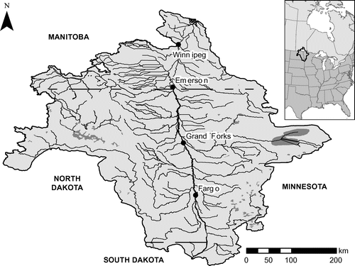
The Red River originates in the US, near the borders of North Dakota, South Dakota and Minnesota (Figure 1), and flows north along the border of North Dakota and Minnesota, entering Manitoba at the town of Emerson about 100 km south of Winnipeg. The basin area south of the Canadian border is approximately 102,000 km². In downtown Winnipeg, the Red River is joined by its main tributary, the Assiniboine River. The Assiniboine River has a basin area that is roughly 33% larger than the Red River basin below the confluence, but because of the relatively low average precipitation in the Assiniboine watershed and extensive withdrawal for irrigation and other water uses, the average annual runoff is only about one third of the total runoff from the combined watershed. Simultaneous flood events on the Assiniboine River and the Red River are relatively rare, and the two river systems are usually treated separately in the analysis of floods. Spring flooding on the Red River is a recurrent concern in Manitoba. The City of Winnipeg is protected by an extensive dike system and the Red River floodway that is used to direct water around the city during significant flood events. The 47-km floodway was recently expanded to a 700-year design capacity and has protected Winnipeg from flooding on many occasions, including the 1997 “flood of the century” event. South of Winnipeg, the smaller communities are protected by ring dikes, and individual properties are either protected by dikes or placed on raised ground. A characteristic of the Red River valley is the extremely low gradient, both along the main channel and of the adjacent land. During severe floods, this results in the inundation of large areas, causing damage to agricultural businesses and transportation infrastructure, as well as significant inconvenience for people living in the floodplain. A detailed description of the 1997 flood and Winnipeg's flood protection system is provided respectively by Rannie (2015) and Blais et al. (this issue).

Figure 1. Red River basin.

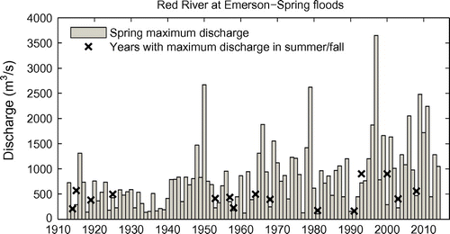
One of the longest continuous records of Red River flows is from the hydrometric station at Emerson at the US border. Figure 2 shows the time series of maximum spring discharge at Emerson for the period 1913 to 2014. Most of the observed maximum annual flows are the result of snowmelt in the spring, and occur in April or early May. In the 102-year record, there are 15 occurrences where summer storms produced flows that exceeded the peak of the spring freshet. As seen in Figure 2, these events are relatively small and more symptomatic of the lack of significant spring runoff than of large summer events. The first part of the record, from 1913 to the mid-1940s – with perhaps the exception of 1916 – is characterized by quite small maximum annual discharge. There were, of course, major floods before 1913, including several large flood events in the nineteenth century (Rannie 1998). The largest flood about which we have somewhat accurate information occurred in 1826. The flood in 1852 has also been estimated to be larger in magnitude than the 1997 flood. Although the exact magnitudes of the pre-record floods are not available, various statistical methods have been devised to include such information in a flood frequency analysis; see for example Benito et al. (2004).

Figure 2. Spring peak discharge for the Red River at Emerson for the period 1913–2014. Years where the maximum annual flow did not occur in the spring are indicated with markers.

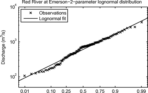
It is not a specific objective of this paper to perform a detailed flood frequency analysis for the Red River where all pertinent information is accounted for. A number of engineering studies have done that. The main interest here is to examine what kind of changes one might expect to see in the distribution of floods under climate change. For reasons explained in the next section, we will employ the two-parameter lognormal distribution to represent spring floods on the Red River. Figure 3 shows that the lognormal distribution provides a good fit to observed spring peak flows on the Red River at Emerson.

Figure 3. Two-parameter log-normal distribution fitted to spring peak flows at Emerson.

The main factors influencing spring floods in the Red River basin are soil moisture at the time of freeze-up in the preceding fall, the winter snow accumulation and rainfall during the spring freshet. Other factors may also play a role, notably the temperature during the melt period and the timing of peak runoff on the tributaries. Alf Warkentin, former chief flood forecaster in Manitoba, compiled a data set of predictor variables with strong links to spring floods on the Red River (Warkentin 1999). The data set is reproduced in Table 1 and covers the period 1940–1999. It includes the following variables:

•	API (antecedent precipitation index): index of soil moisture at freeze-up during the previous autumn, based on weighted basin precipitation from May to September;
•	WP (winter precipitation): total average basin precipitation from 1 November of the previous year to the start of active melt (inches);
•	SP (spring precipitation): total basin precipitation from the start of active spring melt to the date of the spring crest at Emerson (inches);
•	MI (melt index): average degree-days per day at Grand Forks during the active melt period (in Fahrenheit);
•	TF (timing factor): an index of the south–north time phasing of the runoff based on the percentage of tributary peaks experienced on the date of the main stem peak at specific points from Halstad to Winnipeg.

Table 1. Table of flood predictors used in the study.

Year	API	MI	WP	SP	TF	Qpeak
1940	1.87	6.3	1.85	0.98	55	413
1941	2.17	8.0	3.50	1.89	50	787
1942	3.52	6.6	3.23	0.24	60	790
1943	2.23	5.4	4.29	0.04	68	835
1944	2.08	8.4	1.97	0.20	55	348
1945	2.90	8.8	3.90	1.03	44	833
1946	2.09	7.8	2.87	0.73	37	682
1947	2.68	4.7	2.60	2.02	57	804
1948	2.38	8.2	4.61	1.46	64	1470
1949	1.71	9.9	4.09	0.12	78	827
1950	2.71	8.6	4.80	4.06	20	2670
1951	2.19	6.3	3.39	0.24	63	753
1952	2.22	6.9	3.35	0.38	55	685
1953	1.59	9.1	2.91	0.08	36	225
1954	2.14	4.9	2.95	0.00	68	326
1955	2.09	12.9	2.64	0.31	65	663
1956	2.06	6.6	4.02	0.94	61	954
1957	2.24	13.2	2.68	0.20	57	351
1958	2.99	11.3	2.05	0.28	58	174
1959	1.72	10.4	3.15	0.15	44	445
1960	2.78	5.1	2.28	1.26	81	864
1961	2.02	5.3	2.17	0.20	12	121
1962	2.45	3.7	3.82	0.71	36	943
1963	2.59	4.2	1.97	1.34	28	388
1964	1.61	6.1	2.44	1.81	52	481
1965	2.35	5.8	2.52	2.64	35	1310
1966	3.06	6.0	6.18	0.15	12	1880
1967	2.12	9.1	3.46	0.43	67	940
1968	1.50	4.4	3.19	0.04	48	244
1969	2.68	14.9	4.21	1.14	57	1550
1970	2.27	6.9	3.50	2.44	47	1120
1971	2.13	4.6	3.50	0.00	55	753
1972	3.24	6.7	3.35	0.88	70	869
1973	2.10	5.4	2.44	0.39	28	402
1974	3.03	10.1	3.35	2.01	63	1230
1975	2.04	7.3	4.13	2.72	63	1210
1976	2.29	11.4	3.62	0.12	50	886
1977	1.02	11.1	3.27	0.00	19	126
1978	2.95	7.0	4.29	0.94	53	1420
1979	2.03	18.0	4.88	2.89	47	2620
1980	1.86	8.0	3.03	0.00	41	614
1981	2.57	6.0	2.52	0.00	12	107
1982	2.88	3.1	4.09	0.47	37	963
1983	3.18	3.0	3.70	0.08	75	714
1984	2.61	7.3	3.46	0.01	21	855
1985	2.64	8.3	2.48	0.00	50	472
1986	2.70	5.4	3.15	0.55	60	969
1987	2.29	8.6	4.17	0.00	48	1060
1988	2.02	7.5	2.99	0.00	30	444
1989	1.81	3.5	4.96	0.70	43	1200
1990	1.77	3.6	3.19	0.16	30	155
1991	1.75	3.0	2.36	0.06	30	141
1992	2.82	5.4	3.11	0.07	44	445
1993	2.06	9.0	3.66	0.16	51	720
1994	2.50	7.0	3.94	0.15	55	761
1995	3.20	11.0	4.49	0.00	35	1200
1996	2.89	10.0	4.88	0.12	75	1870
1997	2.49	11.6	8.60	0.10	62	3650
1998	2.82	2.7	3.70	0.00	28	780
1999	2.96	9.0	4.69	1.38	44	1660

Note:

API = antecedent precipitation index, MI = melt index, WP = winter precipitation, SP = spring precipitation, TF = timing factor. Qpeak is the spring peak flow at the hydrometric station at Emerson. Detailed definitions of the predictors are given in the main text.

These variables can be related through regression analysis to spring peak discharge on the Red River. It is reasonable to assume that the regression error variance increases with discharge, so some form of variable transformation should be done to satisfy the requirement of linear regression analysis. A logarithmic transformation of dependent and independent variables is used here. Because some years have zero precipitation in the spring, winter and spring precipitation are added in the model:

(1)

where in this study ln  refers to the spring peak discharge at Emerson. The above expression corresponds to a regression function of the form

(2)

This is similar to the model employed by Warkentin (1999), except that he used the discharge at the James Avenue station in Winnipeg rather than at Emerson, and employed nonlinear regression to determine the parameters. The parameters of Equation (1(1) ) can be estimated using standard linear regression. Stepwise regression shows that the variable MI is not significant in the model, and it is therefore not included here. This leads to the following regression relationship:

(3)

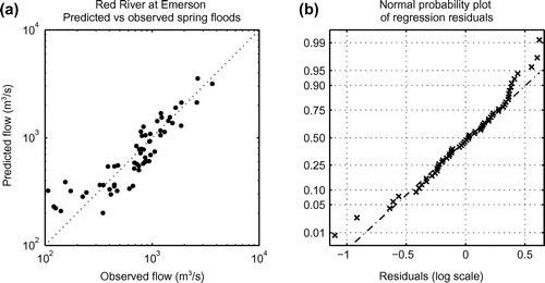
where is assumed to have a normal distribution with constant variance. Figure 4 shows that these assumptions are reasonably satisfied. The adjusted R-square value for the above model is 0.83. It should be noted that as a flood forecasting tool, the regression model may not be quite as effective as suggested by the relatively high R-square value. The predictor variables SP and TF will typically only be fully known during or even after the actual flood, leaving little lead time to act. Nonetheless, as a tool for understanding how climatic factors influence floods in the Red River basin, the regression model in Equation (3(3) ) is useful, and it will be employed for climate change projection in the next section.

Figure 4. Performance of the flood prediction model in Equation (3(3) ) for the period 1940–1999. (a) Predicted versus observed spring peak discharge at Emerson. (b) Normal probability plot of residuals from the regression model in Equation (3(3) ).

Climate change flood scenarios for the Red River

Equation (3(3) ) provides a means to assess changes in the statistical characteristics of floods as a result of changes in the predictor variables. A common assumption in climate change studies is that a model estimated from historical data will apply equally in the future. For Equation (3(3) ), this implies that the regression coefficients and the error variance will remain unchanged. However, the statistical characteristics of the predictor variables may change. Perhaps the most common use of climate model data is the calculation of change factors based on control and future climate scenarios. For precipitation, this involves taking the ratio of future mean values of precipitation and mean values for the control run – typically on a monthly basis – and subsequent scaling of historically observed values with the computed ratios. This approach is alternately called the change factor method or the delta method. The usefulness of the method resides in the fact that it eliminates, or at least reduces, the impact of bias in climate models by considering only relative changes between simulated future and simulated current conditions. In addition, the change factor method is relatively transparent and easy to understand. While more advanced downscaling methods are available, the change factor method is particularly suitable in this study. This is because the climate variables of interest here (API, WP, SP) are highly aggregated both in the temporal and spatial dimension. For the model used here, it is not obvious that advanced downscaling techniques would produce more accurate information beyond what can be gathered from the global climate model simulations.

The procedure used in the following involves finding change factors for the predictor variables API, WP and SP in Equation (3(3) ) and evaluating the implication on the statistics of the dependent variable. There is no reason to suspect that the statistical characteristics of the timing factor TF would change dramatically in the future, and the historical TF values are therefore used in the simulation of future flood distributions. Of particular interest here are the mean value and the variance of ln  which will be used to determine flood frequency distributions for future climates. Consider for a moment a generic regression model of the form

(4)

For a given set of observations, , the parameters can be estimated by the method of least squares. Assuming that the parameters in the above expression have been obtained in this way, it is known from the theory of regression that the following relationships apply:(5) (6) (7)

where the hat indicates values predicted by the model and the overbar indicates mean value. The last two expressions may be written more succinctly as(8) (9)

where E and V are mean and variance operators, respectively. Equation (9(9) ) assumes that all variances, including the variance of the regression error, are calculated as sample variances by dividing by . For a new set of predictor variables, , Equations (8(8) ) and (9(9) ) can be used to estimate the mean value and variance of the dependent variable. Note that to obtain the variance of the dependent variable it is not sufficient to simply calculate the variance of the predicted values; the variance of the error term must be added. In the present context, Equations (8(8) ) and (9(9) ) provide a means to obtain the mean value and variance of in Equation (3(3) ).

The proposed procedure for generating future flood frequency distributions can be summarized as follows:

(1)	Determine delta values for the predictor variables API, WP and SP in Equation (3(3) ) from climate model data. The procedure for this is explained below.
(2)	Modify the observed time series of API, WP and SP in Table 1 using the delta values.
(3)	Use the modified series of API, WP and SP to generate a time series of using Equation (3(3) ), with set to zero.
(4)	Use Equations (8(8) ) and (9(9) ) to determine the mean value and variance of .
(5)	Since, from the regression assumptions, has a normal distribution, the mean value and variance from the previous point represent the parameters of a two-parameter lognormal distribution of floods in the future climate.

The delta values for the three predictor variables are obtained as described below.

API

The antecedent precipitation index is based on a weighted average of basin precipitation from May to October. In calculating the delta factor for API, an exponential filter is used to weight delta values for each month in the period, giving higher weights to months closer to the start of the freezing period. It is necessary to take into account that any change in average precipitation may be modulated by a change in evapotranspiration. One expects that in a generally warmer climate, the evapotranspiration will increase. To calculate the delta value for the API, the following formula is used:(10)

where index i refers to calendar month, overbar indicates mean values, P and E are precipitation and evaporation, respectively, and superscripts “fut” and “con” refer to future values and control period values. is the weight associated with month i, which in the present context is defined as(11)

where c is a constant chosen so that the sum of the weights over the five months equals 1. The highest weight is then given to the change in the month of October and the smallest weight is given to the month of May.

WP

As previously discussed, WP is by definition the precipitation from 1 November to the start of the active melt period. The duration thus varies from year to year. For the calculation of delta factors for WP, it is sufficient to define a fixed period, chosen here to be the period from November to March. In a generally warmer climate, the period of snow accumulation will be shorter, and this must be taken into account in the evaluation of the delta factors. The following formula is used to calculate the delta factors for WP:

(12)

where the overbars refer to averages over the winter months (November to March, averaged over all years), and D refers to the average duration of the below-zero period. For example, if the below-zero period is on average 10% shorter in a future climate, one would expect – everything else being equal – a 10% reduction in the average accumulated snow pack. The average duration of the below-zero period is calculated from the monthly mean temperatures from the different climate models. Linear interpolation is used to find the Julian day in the late fall and early spring where the mean temperature is zero. This information can be used to determine the average below-zero period. Equation (12(12) ) also takes into account that evaporation during winter may be different in the future and could affect the total snow accumulation.

SP

Delta values for spring precipitation are calculated as (13)

where the averages are calculated over the months of April and May. Changes in evaporation are assumed to be unimportant here since the temperatures in current and future climates can reasonably be assumed to be similar during the melt period. Of course, in a warmer climate, the melt period would start earlier.

Once the delta values have been obtained from the model data, new values of the predictor variables can be calculated by multiplying the numbers in Table 1 by the delta values:

(14)

These values can then be used to generate new flood distributions following the procedure described earlier in this section.

The climate model data used in the study were obtained from the Coupled Model Intercomparison Project – Phase 5 (CMIP5) multi-model ensemble (Taylor et al. 2012). The CMIP5 is an updated version of CMIP3, and was the basis for part of the material presented in the Fifth Assessment Report of the Intergovernmental Panel on Climate Change (IPCC) (Hartman et al. 2013). The monthly data were downloaded from the Earth System Grid Federation (ESGF) portal. Although many models are included in the CMIP5 archive, not all have the data required for this study. Table 2 provides a list of the 16 climate models used in this investigation. The control climate was based on the 30-year period from 1971 to 2000. Two future periods were considered: the period 2031–2060 and the period 2071–2100. As for climate scenarios, two Representative Concentration Pathways, the RCP4.5 and RCP8.5, were considered. These are the ones with the most data available in the CMIP5 data set. The RCPs replace the scenarios that were used in the Fourth Assessment Report of the IPCC. The numbering of RCPs refers to the increase in radiative forcing in 2100 relative to pre-industrial levels. For example, RCP4.5 indicates an increase of radiative forcing of +4.5W/m² in year 2100. The RCP8.5 is the most severe of the four RCP scenarios.

Table 2. Global climate models from the Coupled Model Intercomparison Project – Phase 5 (CMIP5) ensemble used in the study.

Modeling center (or group)	Institute ID	Model name
Beijing Climate Center, China Meteorological Administration	BCC	BCC-CSM1.1(m)
Canadian Centre for Climate Modelling and Analysis	CCCMA	CanESM2
National Center for Atmospheric Research	NCAR	CCSM4
Community Earth System Model Contributors	NSF-DOE-NCAR	CESM1(BGC)
Centro Euro-Mediterraneo per I Cambiamenti Climatici	CMCC	CMCC-CM
Centre National de Recherches Météorologiques/Centre Européen de Recherche et Formation Avancée en Calcul Scientifique	CNRM-CERFACS	CNRM-CM5
LASG, Institute of Atmospheric Physics, Chinese Academy of Sciences and CESS, Tsinghua University	LASG-CESS	FGOALS-g2
Meteorological Office Hadley Centre (additional HadGEM2-ES realizations contributed by Instituto Nacional de Pesquisas Espaciais)	MOHC(additional realizations by INPE)	HadGEM2-CCHadGEM2-ES
Institute for Numerical Mathematics	INM	INM-CM4
Japan Agency for Marine-Earth Science and Technology, Atmosphere and Ocean Research Institute (The University of Tokyo), and National Institute for Environmental Studies	MIROC	MIROC-ESMMIROC-ESM-CHEM
Atmosphere and Ocean Research Institute (The University of Tokyo), National Institute for Environmental Studies, and Japan Agency for Marine-Earth Science and Technology	MIROC	MIROC5
Max-Planck-Institut für Meteorologie (Max Planck Institute for Meteorology)	MPI-M	MPI-ESM-MRMPI-ESM-LR
Meteorological Research Institute	MRI	MRI-CGCM3

For each of the models considered in the study, the grid point closest to the centroid of the part of the Red River basin south of the Canada–US border was identified. Data are typically provided at a resolution of 1 to 2 degrees, and it was deemed unnecessary to perform any spatial interpolation or averaging of grid values as the differences in climate statistics from a grid cell to neighbouring grid cells are relatively small. For each of the models, monthly precipitation, temperature and evaporation values for the control period (1970–1999) and the two future periods (2031–2060 and 2071–2100) were extracted. This was done for the two climate scenarios RCP4.5 and RCP8.5.

Results

Figure 5 shows a scatter plot of the delta values for annual precipitation and annual mean temperature in the Red River basin for the 16 climate models considered in the study, and for the two time periods and two emission scenarios. All models agree that temperature will increase in the future and, as expected, the changes are more significant for RCP8.5 compared to RCP4.5, as well as more severe for the period 2071–2100 than for the 2031–2060 period. In the RCP8.5 scenario, one should expect mean temperature increases in the order of 6–9 degrees by the end of this century, whereas under the more moderate RCP4.5 scenario temperatures could rise by 3–5 degrees by the end of the century. As seen in Figure 5, there are quite large differences in the predicted effects of higher greenhouse gas concentration. A closer examination of the monthly mean values from model simulations suggests that temperature increases are fairly consistent throughout the year (Figure 6a). The implication of the warmer weather is a generally shorter winter season. Based on the climate normals for Grand Forks in North Dakota, the average period with mean temperatures below 0°C is 143 days. Depending on the scenario and time period, the typical below-zero period is expected to decrease in duration by 10–20%, shortening the effective time of snow accumulation.

Figure 5. Delta values for annual precipitation and mean annual temperature in the Red River basin. For precipitation (P), delta values represent the ratio of the mean of future annual precipitation (average of the 30-year periods) to the mean of annual precipitation for the control simulation. For temperature (T), delta values represent differences between future mean annual temperature and control mean annual temperature. The points correspond to the 16 global climate models listed in Table 2. RCP = Representative Concentration Pathways.

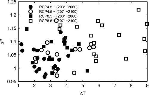
Figure 6. Monthly ensemble means of control simulation and future simulations for (a) temperature, (b) precipitation and (c) evaporation. Each curve is obtained by averaging over the 16 global climate models in Table 2.

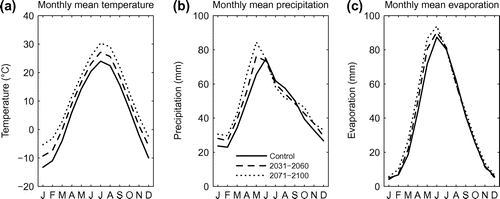
There is considerably more inter-model variability in the prediction of changes in mean annual precipitation. The various experiments do not all agree on the sign of change, but in the large majority of cases, there is evidence that annual precipitation will increase in the future. One can generally conclude that the increases are higher with the more severe RCP8.5 scenario, and larger toward the end of the century compared to the middle of the century. Under the RCP8.5 scenario, one would expect an increase in annual precipitation in the order of 5–10% for the 2031–2060 period, while at the end of the century annual precipitation may increase by roughly 10–20%. This observation is consistent with the general expectation that annual precipitation will increase with warmer temperatures in the region. As seen in the model composite results in Figure 6b for the RCP8.5 scenario, the increase in annual precipitation is primarily due to an increase in winter precipitation, whereas there is little or no change in the summer months. From a runoff perspective, the increase in winter precipitation will likely be partly offset by an increase in evaporation (Figure 6c). Evaporation is expected to increase in the winter and spring months, while being relatively unchanged in the later part of the calendar year.

The projected changes in temperature, precipitation and evaporation will impact the predictor variables in the flood prediction model. Figure 7 shows boxplots of the delta values for the three predictor variables API, WP and SP for each of the emission scenarios and each time period. The API does not appear to be changing significantly in any particular direction, although on average there appears to be a slight increase. This is consistent with the previous conclusion that precipitation and evaporation in the fall on average (over models) are not expected to change significantly. The WP variable is likely to decrease in future years. Although mean monthly precipitation is expected to increase, the delta values for WP take into account the possible offset by higher evaporation rates and the generally shorter snow accumulation period. For most models, the net effect is a decrease in WP, although a couple of models are seen to produce rather high increases in WP (outliers indicated in the box plot).

Figure 7. Change factors for flood predictors used in the regression model in Equation (3(3) ). The box plots are based on the 16 global climate models in Table 2 and are calculated using Equations (1(1) 0), (12) and (13). RCP = Representative Concentration Pathways.

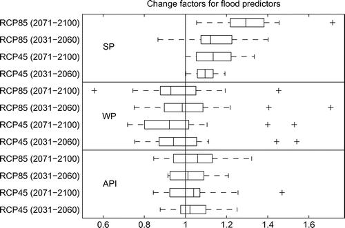
The most significant change in predictor variables is in the variable SP, with virtually all models indicating an increase. Although delta values for SP are quite high compared to the delta values for WP, it should be kept in mind that the numerical values of WP are generally larger than SP, so changes in WP may therefore still have a more significant impact on flood distributions.

The methodology described previously was applied to generate flood distributions for the Red River under current and changed climate conditions. The results are reported in Figure 8. The figure shows the results obtained from each of the 16 climate models in grey scale, for each of the emission scenarios and each time period. The average and median of the models are also presented in the figure. As can be seen, two models produce flood quantiles that are significantly higher than the others. They correspond to the outlying WP delta values in Figure 7. There is always a possibility that some models produce results that are dramatically different from the bulk of other models. That is why one might prefer to consider the median of model results rather than the mean value. The median is generally less sensitive to outliers than the mean value.

Figure 8. Projected changes in the distribution of floods for different emission scenarios and different time periods. Grey lines show the results from individual global climate models. RCP = Representative Concentration Pathways.

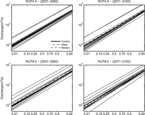
From Figure 8, it can be seen that while individual climate models may suggest significant changes in flood distributions both in the direction of more severe and less severe floods, there is little difference between the median of the model ensemble and the control run. The variability of the individual model results is a measure of model uncertainty, and highlights the difficulty in assessing the impact of climate change on extreme events such as floods. Based on the present study, there is insufficient evidence to suggest a particular direction of change in the distribution of floods on the Red River. What one can conclude is that changes are likely to happen, but whether they will be in the form of more frequent or less frequent floods is impossible to say.

Conclusions

In this study, a simple regression-based flood prediction model has been used to investigate the impact of climate change on the distribution of floods in the Red River basin. An alternative approach would be the use of continuous hydrologic models with future climate data derived from downscaling of global climate model output. For the particular case of the Red River basin, it is not evident that the use of a hydrologic model would produce superior results. First of all, as discussed in the paper, the regression-based model performs quite well and is specifically designed to estimate flood peaks. To perform well, a continuous hydrologic model must reproduce a range of other flow characteristics and may not estimate peak flows any better than the regression model. The regression model uses spatially and temporally integrated predictor variables, and to obtain information about changes to the predictor variables, it does not seem unreasonable to rely directly on the output from global climate models which have a spatial resolution of the same order of magnitude as the Red River basin. This eliminates the need for temporal and spatial downscaling that can introduce new uncertainties but would be required for continuous hydrologic modelling. The possible advantage of using a hydrologic model is that certain processes that may influence spring peak runoff can be explicitly modelled. For example, in a future warmer climate there may be more frequent occurrences of liquid precipitation events during the winter, which may have an impact on antecedent soil moisture at the start of the spring freshet.

A number of studies of climate change impacts on hydrology have concluded that the largest sources of uncertainty are the global climate models and the emission scenarios. While little can be done to reduce the uncertainty in emission projections, which necessarily involve hypotheses about things such as future population growth and environmental policies, climate models are continuously being improved, resulting in increasing accuracy. However, at present, there are still rather significant discrepancies between models. It is therefore imperative to use ensembles of climate models when assessing the impact of climate change on, for example, flood frequency. Ensemble results provide a framework for quantifying the uncertainty in future projections, and should be useful for decision makers. For the specific case of the Red River basin and the methodology employed in this paper, the main conclusion is that changes are likely to happen, but there is insufficient evidence to suggest a particular direction of the change.

Acknowledgements

The climate data used in this study were provided by the World Climate Research Programme's Working Group on Coupled Modelling, which is responsible for the CMIP initiative. The data were extracted and compiled by Scott Pokorny; the author gratefully acknowledges his assistance.

References

- Ahmad, S., and S. P. Simonovic. 2005. An artificial neural network model for generating hydrograph from hydro-meteorological parameters. Journal of Hydrology 315(1): 236–251.
- Benito, G., M. Lang, M. Barriendos, M. C. Llasat, F. Francés, T. Ouarda, and B. Bobée. 2004. Use of systematic, palaeoflood and historical data for the improvement of flood risk estimation. Review of scientific methods. Natural Hazards 31(3): 623–643.
- Blais, E., S. Clark, K. Dow, B. Rannie, T. Stadnyk., and L. Wazney. This issue. Background to flood control measures in the Red and Assiniboine River Basins. Canadian Water Resources Journal. doi:10.1080/07011784.2015.1036123.
- Booy, C., and D. R. Morgan. 1985. The effect of clustering of flood peaks on a flood risk analysis for the Red River. Canadian Journal of Civil Engineering 12(1): 150–165.
- Burn, D. H., and A. Taleghani. 2013. Estimates of changes in design rainfall values for Canada. Hydrological Processes 27(11): 1590–1599.
- Bush, E. J., J. W. Loder, T. S. James, L. D. Mortsch, and S. J. Cohen. 2014. An overview of Canada’s changing climate. In Canada in a changing climate: Sector perspectives on impacts and adaptation, eds. F. J. Warren and D. S. Lemmen, 23–64. Ottawa: Government of Canada.
- Eum, H. I., and S. P. Simonovic. 2012. Assessment on variability of extreme climate events for the Upper Thames River basin in Canada. Hydrological Processes 26(4): 485–499.
- Hartmann, D. L., A. M. G. Klein Tank, M. Rusticucci, L.V. Alexander, S. Brönnimann, Y. Charabi, F.J. Dentener, et al. 2013. Observations: Atmosphere and surface. In Climate change 2013: The physical science basis. Contribution of Working Group I to the Fifth Assessment Report of the Intergovernmental Panel on Climate Change, ed. T. F. Stocker, D. Qin, G.-K. Plattner, M. Tignor, S. K. Allen, J. Boschung, A. Nauels, et al., 159–254. Cambridge, UK and New York: Cambridge University Press.
- Hassanzadeh, E., A. Nazemi, and A. Elshorbagy. 2013. Quantile-based downscaling of precipitation using Genetic Programming: Application to IDF curves in Saskatoon. Journal of Hydrologic Engineering 19(5): 943–955.
- Mailhot, A., I. Beauregard, G. Talbot, D. Caya, and S. Biner. 2012. Future changes in intense precipitation over Canada assessed from multi-model NARCCAP ensemble simulations. International Journal of Climatology 32(8): 1151–1163.
- Mailhot, A., S. Duchesne, D. Caya, and G. Talbot. 2007. Assessment of future change in intensity–duration–frequency (IDF) curves for Southern Quebec using the Canadian Regional Climate Model (CRCM). Journal of Hydrology 347(1): 197–210.
- Rannie, W. F. 1998. A survey of hydroclimate, flooding, and runoff in the Red River basin prior to 1870. Winnepeg, MB: University of Winnipeg.
- Rannie, W. F. 2015. The 1997 flood event in the Red River basin: Causes, assessment, and damages. Canadian Water Resources Journal. doi:10.1080/07011784.2015.1004198.
- Simonovic, S. P., and R. W. Carson. 2003. Flooding in the Red River Basin: Lessons from post flood activities. Natural Hazards 28(2–3): 345–365.
- Simonovic, S. P., and L. Li. 2004. Sensitivity of the Red River Basin flood protection system to climate variability and change. Water Resources Management 18(2): 89–110.
- St. George, S., and E. Nielsen. 2003. Palaeoflood records for the Red River, Manitoba, Canada, derived from anatomical tree-ring signatures. The Holocene 13(4): 547–555.
- Taylor, K. E., R. J. Stouffer, and G. A. Meehl. 2012. An overview of CMIP5 and the experiment design. Bulletin of the American Meteorological Society 93: 485–498. doi:10.1175/BAMS-D-11-00094.1.
- Trenberth, K. E. 2011. Changes in precipitation with climate change. Climate Research 47(1): 123–138. doi:10.3354/cr00953.
- Vincent, L. A., X. L. Wang, E. J. Milewska, H. Wan, F. Yang, and V. Swail. 2012. A second generation of homogenized Canadian monthly surface air temperature for climate trend analysis. Journal of Geophysical Research 117: D18110.
- Warkentin, A. A. 1999. Red River at Winnipeg, hydrometeorological parameter generated floods for design purposes. In Proceedings of Red River Flooding Decreasing our Risk, Canadian Water Resources Association, Winnipeg, October 27–28, 1999.
- Willett, K. M., P. D. Jones, N. P. Gillett, and P. Thorne. 2008. Recent changes in surface humidity: Development of the Had-CRUH dataset. Journal of Climate 21: 5364–5383.