Modeling of subsurface agricultural drainage using two hydrological models with different conceptual approaches as well as dimensions and spatial scales

Abstract

In regions where soils are seasonally or perennially wet, subsurface drainage represents an essential water management practice. Two hydrological models with different modeling approaches as well as different dimensional and spatial scales, DRAINMOD (1D, lumped and field-scale) and CATHY (3D, spatially distributed and watershed-scale), were compared in terms of their performance to predict tile-drain flow and to simulate evapotranspiration (ET) under field conditions. Two metrics were defined to assess the capacity of the models to represent the soil water dynamics: relative errors in simulating peak flow and drainage volume. Using different hydraulic conductivity scenarios, both models provided similar results. For the total predicted/observed tile-drain flow comparison, the two models yielded very similar results. In terms of coefficient of determination (R²) and Nash–Sutcliffe model efficiency (NSE), their performances were low in simulating tile-drain flows for dry periods (low observed tile-drain flow). During periods with higher observed tile-drain flow, the performance of both models was good (R² > 0.75 and NSE mostly > 0.60), but DRAINMOD produced better results than CATHY did. The two models had similar ET values (R² > 0.80). Regarding the impact of the hydraulic conductivity of each soil layer on subsurface drainage outflow, this study showed that the soil layer below the tile-drain system was the most influential for the two models.

Dans les régions où les sols sont saisonnièrement ou perpétuellement humides, le drainage souterrain agricole représente une pratique essentielle de gestion de l’eau. Deux modèles hydrologiques avec différentes approches de modélisation ainsi que différentes échelles dimensionnelles et spatiales, DRAINMOD (1D, localisé et à l’échelle du champ) et CATHY (3D, spatialement distribué et à l’échelle de bassin versant), ont été comparés en fonction de leur performance pour prédire l’écoulement aux drains et à simuler le processus d’évapotranspiration dans des conditions de terrain. Deux mesures ont été définies pour évaluer la capacité des modèles à représenter la dynamique de l’eau dans le sol: les erreurs relatives à simuler le débit de pointe et le volume de drainage. En utilisant différents scénarios de conductivité hydraulique, les deux modèles ont fourni des résultats similaires. Vis-à-vis de la comparaison d’écoulement total drainé simulé/observé, les deux modèles ont donné des résultats très similaires. En termes de coefficient de détermination (R²) et le coefficient d’efficacité de Nash-Sutcliffe (NSE), pendant les périodes sèches (faible débit observé aux drains souterrains) leurs performances ont été faibles en simulant l’écoulement aux drains souterrains. Pendant les périodes d’écoulement observé aux drains plus élevé, la performance des deux modèles était bonne (R² > 0,75 et NSE généralement > 0,60), mais DRAINMOD produit de meilleurs résultats que CATHY. Les deux modèles ont bien simulé le processus d’évapotranspiration (R² > 0,80). En ce qui concerne l’impact de la conductivité hydraulique de chaque couche de sol sur l’écoulement sortant de drains souterrains, cette étude a montré que la couche de sol sous le système des drains souterrains était la plus influente pour les deux modèles.

Introduction

Subsurface drainage is a common agricultural practice to improve aeration and trafficability of soil in regions characterized by seasonal high water tables (Eggelsmann 1981; Skaggs et al. 1994). When installing an agricultural subsurface drainage system, farmers do so for two major reasons: (1) agricultural drainage systems usually increase crop yield of poorly drained soils by providing a better environment for plant growth, especially during wet periods; and (2) drainage systems generally improve field conditions for timely tillage, planting and harvesting.

When subsurface drains are in place, the drainable water fraction of the soil profile is converted to short-term (detention) storage over a period of few hours, days or weeks, depending on a number of variables. These include tile drain size, depth and spacing, soil type, outlet size/condition, and whether or not under continuous rainfall or snowmelt conditions. When drainable water is removed from the soil profile, infiltration can then occur. This is due to available soil pore space allowing water that would otherwise be stored in the surface depressions to infiltrate and have a direct pathway to downstream flow via the subsurface drains (BTSAC 2012).

Although agricultural production has benefited from agricultural drainage in many regions and countries, there are concerns about potential environmental impact (e.g. St-Hilaire et al. 2015). The most dramatic hydrological changes in a landscape occur when the latter is converted from native vegetation to intensive cropping systems. When tile drains are implemented, they can substantially alter the total water yield from a field or small watershed as well as modify the timing and shape of the hydrograph (Schilling and Helmers 2008). Tile drainage increases the proportion of annual precipitation that is discharged to surface waters via subsurface flow relative to the amount that is stored, evaporated or transpired (Serrano et al. 1985; Magner et al. 2004; Tomer et al. 2005).

In several studies across the midwestern United States and Canada, discharge from tile drains constitutes the majority of stream flow in many agricultural watersheds. King et al. (2014) found that tile drainage contributed 51% of annual stream flow in a headwater watershed in Ohio. Meanwhile, in a watershed in Ontario, Canada, it was estimated that 42% of annual watershed discharge originated from tile flow (Macrae et al. 2007). Culley and Bolton (1983) and Xue et al. (1998) also estimated that 60 and 86%, respectively, of stream flow was derived from tile drains. Although total water yield from a field tends to increase with the installation of subsurface drainage, surface runoff and sediment yield are often significantly decreased (Istok and Kling 1983; Skaggs et al. 1994; Robinson and Rycroft 1999; Dolezal et al. 2001). Subsurface drainage reduces both peak outflows and the frequency of surface runoff events at sites characterized by high water tables or prolonged surface saturation (“ponding”) under undrained conditions (Robinson 1990; Robinson and Rycroft 1999).

The main water quality concern about subsurface drainage is the increased loss of nitrates and other soluble constituents (i.e. pesticides, dissolved phosphorus, to name a few) that can move through soils and end up in nearby surface waters. It is therefore generally agreed that the installation of subsurface drainage decreases the amount of phosphorus and soil lost in surface runoff because the volume of surface runoff is reduced (Bengtson et al. 1995; Zucker and Brown 1998). Phosphorus loss via artificial drainage has been shown to contribute to the accelerated eutrophication of rivers, lakes, estuaries and even coastal waters, including some of the most challenging cases of agriculturally derived eutrophication (Kleinman et al. 2015). The installation of artificial drainage not only increases peak flows, which accounts for the majority of phosphorus loss, but also connects areas of landscape with plumbing and channels where flows were previously more diffuse (King et al. 2015; Smith et al. 2015).

The impact of artificial drainage strongly depends on characteristics of an individual site, that is: topography (slope), drainage system design (spacing, depth and size of drains) and soil type (hydraulic conductivity) (Dunn and Mackay 1996; Holden et al. 2004). The hydrological response of tile drainage during a given event varies based on event characteristics, such as rainfall amount and intensity (Vidon and Cuadra 2011), and antecedent soil moisture conditions (Kung et al. 2000; Dolezal et al. 2001; Macrae et al. 2007).

There have been numerous studies on tile drainage, and various modeling approaches have been proposed such as the classical Hooghoudt equation (Hooghoudt 1940), Kirkham equation (Kirkham 1958), Ernst equation (Ernst 1962), Richards equation (Fipps and Skaggs 1991) and Laplace or Boussinesq equations (Bouarfa and Zimmer 2000). These approaches have been incorporated into several conceptual and distributed models. The Kirkham and Hooghoudt equations are used, for example, in DRAINMOD (Skaggs 1980), while the MACRO (Larsbo and Jarvis 2003) uses the Hooghoudt equation. In SWAP (Kroes et al. 2008), the user has the option of using either the Hooghoudt equation or that of Ernst, depending on the issue under consideration.

Fipps et al. (1986) tested four different methods of tile drain representation in the finite elements solution of the two-dimensional form of Richards’ equation. These methods are: (1) hole approach as drain model, (2) nodal-point approach with specified or imposed flux, (3) imposed pressure-head approach, and (4) resistance-adjustment approach. In the latter method, the conductivity at the drain is adjusted by a factor determined by the ratio between the effective radius of the drain and the size of the elements surrounding the drain node. The problem with methods (1) and (2) is that a large number of nodes are necessary in the vicinity of the drain for more realistic results, while methods (3) and (4) are implemented with coarse grids.

For grids in three dimensions where there are a number of tile drains in the domain, the extremely fine discretization required to represent the small openings (drains) is computationally time consuming (Fipps et al. 1986). In order to get a solution to this problem, a Dirichlet boundary condition (imposed pressure head) or that of Neumann (imposed flux) is generally applied to the nodes representing tile drains. One of these two conditions can be integrated in CATHY (Camporese et al. 2010) to simulate the subsurface drainage system. Using the pressure-head condition implies that the head at the tile drains remains constant throughout the simulation and the flow in the drains is not affected by factors such as the cross section of drains (MacQuarrie and Sudicky 1996). In order to simulate the drainage system in a three-dimensional mesh of the porous matrix, where groundwater flow is governed by the Richards equation, one can distinguish between the following three approaches among others. First, a one-dimensional flow equation is introduced to the tile drain. This is the case of HydroGeoSphere (MacQuarrie and Sudicky 1996; Therrien et al. 2007; Brunner and Simmons 2012) where the flow is based on the continuity equation in an open channel. Next, the subsurface drainage system flow depends on the water height above the drain level and an imposed time constant which is calculated according to the linear reservoir concept. This is the case for MIKE-SHE (DHI 2007). Finally, we may use the equivalent representation of tile drains in the soil profile using an anisotropic homogeneous porous medium. Indeed, as reported by Carlier et al. (2007), this tile-drain representation, when compared to other approaches using the three-dimensional (3D) SWMS code of Simunek et al. (1995), provided acceptable results for global water outflow and mean water table elevation.

To our knowledge, although there are studies dealing with testing (evaluation) and application of CATHY, there are no exhaustive studies on the simulation of the water flow through a subsurface drainage system at the field or watershed scale using this model. On the other hand, the DRAINMOD model is widely used throughout the world to describe the hydrology of poorly or artificially drained soils. Thus, these reasons have guided the selection of these two hydrological models.

Locally based research is necessary to better understand the impact that subsurface drainage can have at the field scale as well as at the catchment scale. The objectives of this study were: (1) to investigate the soil water dynamics using two hydrologic models, DRAINMOD (Skaggs 1978; Skaggs et al. 2012), a one-dimensional (1D), lumped and field-scale model, and CATHY (Camporese et al. 2010), a 3D, spatially distributed and watershed-scale model; (2) to evaluate the ability of CATHY to simulate the water flow through a subsurface drainage system and the evapotranspiration process while comparing the latter with DRAINMOD; and (3) to evaluate the impact of the saturated hydraulic conductivity of each soil layer on the simulated subsurface drainage outflow.

Materials and methods

Description of the hydrologic models

DRAINMOD, a field-scale hydrologic model, was developed to simulate the performance of drainage and related water table management systems on subsurface drainage, water table fluctuations, and yields (Skaggs 1978; Skaggs et al. 2012). CATHY (CATchment HYdrology) is a coupled, physically based and spatially distributed model simulating surface-subsurface flows processes (Camporese et al. 2010).

The following paragraphs provide a description of the two models in terms of their respective approach to simulate surface flow, subsurface flow and tile-drain flow, and main input data and boundary conditions. Detailed descriptions of DRAINMOD and CATHY can be found in Skaggs (1978) and Skaggs et al. (2012); and in Bixio et al. (2000) and Camporese et al. (2010), respectively.

Surface flow

At each computational time step Δt, DRAINMOD computes runoff (RO) [L] using a water balance approach(1)

where P is the precipitation [L], F infiltration [L] and ΔS is the change in volume of water stored on the surface [L]. There is no surface flow routing.

For CATHY, the available water for surface flow, computed using a water balance approach, is routed using the diffusive wave equation describing surface flow propagation over hillslopes and in stream channels identified using terrain topography and the hydraulic geometry concept:(2)

where Q is the discharge along the rivulet/stream channel [L³/T], c_k is the kinematic celerity [L/T], s is the 1D coordinate system [L] describing each element of the drainage network, D_h is the hydraulic diffusivity [L²/T] and q_s is the inflow (positive) or outflow (negative) rate from the subsurface to surface [L³/LT].

Subsurface flow

DRAINMOD is based on a water balance for a section of soil of unit surface area that extends from the impermeable layer to the surface and is located midway between parallel drains. The water balance for a time increment Δt may be expressed as:(3)

where ΔV_a is the change in the water-free pore space or air volume [L], D is drainage from (or subirrigation into) the section [L], ET is evapotranspiration [L], DLS is deep and lateral seepage [L] and F is infiltration [L] entering the section.

For CATHY, the subsurface flow model solves the 3D Richards equation describing flow in variably saturated porous media:(4)

where is relative soil saturation, θ is the volumetric moisture content [L³/L³], ϕ is the porosity [L³/L³], S_s is the aquifer specific storage coefficient [L⁻¹], ψ is pressure head [L], t is time [T], is the gradient operator [L⁻¹], K_s is the saturated hydraulic conductivity tensor [L/T], K_r(ψ) is the relative hydraulic conductivity function [dimensionless], η_z = (0,0,1)^T the unit vector representing vertical flow, z is the vertical coordinate directed upward [L], and q_ss represents distributed source (positive) or sink (negative) terms [L³/L³T].

Tile-drain flow

Under most conditions, the drainage rate for DRAINMOD can be estimated with the steady-state Hooghoudt equation, which is based on the Dupuit-Forchheimer assumptions:(5)

where q is the drainage rate [L/T], m is the midpoint water table elevation above the drain [L], K_e is the equivalent lateral hydraulic conductivity of the profile [L/T], d_e is the equivalent depth from the drain to the restrictive layer [L], and L is the drain spacing [L]. The tile-drain flow for the CATHY model is due to the consideration of zero pressure head (atmospheric pressure) at the nodes delineating the drainage network in the porous media.

Main model input data and boundary conditions

The major difference between the two models is that DRAINMOD is a lumped, 1D model and CATHY is a spatially distributed 3D model which in its current form does not take into account the effective radius, drainage coefficient. As a reminder, according to Moradkhani and Sorooshian (2008) for lumped models, the entire river basin is taken as a single unit where spatial variability is disregarded and hence the outputs are generated without considering the spatial processes, whereas a distributed model can make predictions that are distributed in space by dividing the entire catchment into small units, usually square cells or triangulated irregular network, so that the parameters, inputs and outputs can vary spatially.

As noted above, the simulation domain for DRAINMOD is a section of soil of unit surface area extending from the impermeable layer to the surface and located midway between parallel drains. Precipitation and evapotranspiration are applied at the soil surface (upper boundary conditions), while deep and lateral seepage takes place through the impermeable layer. Considering flow in the saturated zone only, from a drain to its half-distance to nearby drains, the boundary conditions are given by the height of the water table. With respect to the physical domain accounted for by DRAINMOD, the simulation domain for CATHY corresponds to field dimensions along with the following boundary conditions: zero flux for lateral and deep boundaries, while the flux at the soil surface results from the difference between precipitation and evapotranspiration. The atmospheric pressure (zero pressure head) is applied at the nodes delineating the artificial subsurface drainage.

Study site and database source

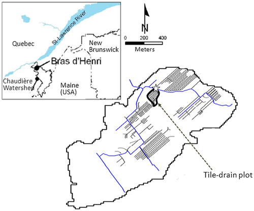
The study site is a 2.44-ha tile-drained plot of a headwater micro-watershed (Figure 1) characterized by intensive livestock production supported by forages and annual crops such as corn grain and soybeans. It is located in the Bras d’Henri watershed, Quebec (Canada), as part of a Canada-wide research program called Watershed Evaluation of Beneficial management practices, WEBs (Yang et al. 2007). This program, launched in 2004, was led by Agriculture and Agri-food Canada (AAC) to measure the environmental and economic impacts of selected agricultural Beneficial Management Practices (BMPs) at the watershed scale.

Figure 1. Location of tile-drained plot of interest in the Bras d’Henri micro-watershed (the star indicates the outlet).

Located in the Quebec Appalachians, the Bras d’Henri watershed is characterized by a rolling relief ranging from 150 to 170 m above mean sea level. The surficial geologic materials were deposited during the presence of the Champlain Sea and consist of thin (< 10 m) littoral sediments overlying clayed glacial diamictons (Gadd 1974). These diamictons generally reach a thickness of 1.0 to 1.5 m, but they are not present throughout the watershed. Soils in tile-drained field have textures ranging from coarse sandy loams to very fine loamy sands. Winters are long and cold, summers are fresh and short with substantial annual precipitation, averaging 1150 mm, where one third accumulates as snow. During summer, precipitation is generally greater than evaporated water, and therefore no water deficit in soils is observed (Lamontagne et al. 2010).

The database provided by AAC includes meteorological data (mean air temperature, maximum and minimum air temperatures, relative humidity, saturation vapour pressure at air temperature, wind speed at height of 2 m, net radiation at the crop surface, precipitation, vapour pressure), and hydraulic properties (hydraulic conductivity, porosity, water content) obtained by suction test from the soil surface up to 1.25 m depth. Saturated hydraulic conductivity in the horizontal direction was inferred from vertical saturated hydraulic conductivity. The horizontal, saturated, hydraulic conductivity at depths greater than 1.25 m was obtained from slug-tests, from which vertical saturated hydraulic conductivity was derived.

Assessment of soil water dynamics

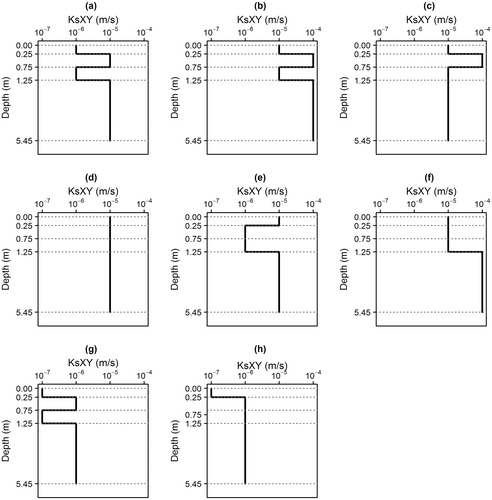
This section provides the necessary background on the saturated hydraulic conductivity (KsXY) values that were used to corroborate as well as possible the observed tile-drain flows. Figure 2 presents eight scenarios of lateral saturated hydraulic conductivity. The KsXY values of scenario 1 correspond to those measured at the study tile-drained plot. The KsZ values were maintained constant and equal to those in the horizontal direction of scenario 1 (i.e. KsXY) for all scenarios in the vertical direction with regard to CATHY. The way in which the soil profile was discretized is given in the next section. Simulations for the eight scenarios were done using the 2012 meteorological data. Given that calibration and validation for the two models were done over short periods of 15 days during which observed tile-drain flows were manually recorded, this idealized analysis of DRAINMOD and CATHY was focussed on the 292nd to 307th Julian day of 2012.

Figure 2. Different scenarios of saturated hydraulic conductivity (KsXY) configurations for soil dynamics models assessment: (a) Scenario 1; (b) Scenario 2; (c) Scenario 3; (d) Scenario 4; (e) Scenario 5; (f) Scenario 6; (g) Scenario 7; and (h) Scenario 8.

Model inputs

Soil properties – CATHY

The 3D subsurface computational domain for the tile-drained field was constructed from a 20-m resolution digital elevation model (DEM). Each DEM cell was subdivided into two triangles. The resulting two-dimensional (2D) surface mesh pattern of 140 nodes, among which 59 nodes were above the tile-drain network, was then used to subdivide a 5.45-m porous media into 15 soil layers. Nodes delineating the subsurface drainage network were located between the eighth and ninth layers at 1.15 m below soil surface. The thinnest layers were placed at the surface and around the drainage network to accurately resolve the partitioning of the rainfall-runoff process or to better capture the interactions between surface water and groundwater, and to properly take into account the tile-drain influence on subsurface flow. The resulting 3D grid contained 2240 nodes and 10,530 tetrahedral elements. Table 1 summarizes the values of the physical properties associated with each soil layer, namely, saturated hydraulic conductivity in the horizontal (KsXY) and vertical (KsZ) directions, specific storage (Ss), and porosity (ϕ). Soil hydraulic properties were described by parameters of the van Genuchten and Nielsen (1985) relationships, that is: the fitting parameter (VGN), the residual moisture content (VGRMC) and the air entry pressure head (VGPSAT).

Table 1. CATHY soil hydraulic parameters in the porous media.

Layers	Depth (m)	Thickness (m)	KsXY (cm/h)	KsZ (cm/h)	Ss (m^−1)	ϕ (-)
01–03	0.00–0.25	0.25	16.25	3.25	6.0 x 10^−4	0.48
04–05	0.25–0.75	0.50	97.60	32.5	1.8 x 10^−4	0.48
06–10	0.75–1.25	0.50	16.25	3.25	6.0 x 10^−4	0.41
11–15	1.25–5.45	4.20	25.90	5.18	3.5 x 10^−4	0.45
VGN (-): 4.85 VGRMC (-): 0.105 VGPSAT (-): −0.25

Soil properties – DRAINMOD

The soil profile was divided into four layers as shown in Table 2. The unsaturated hydraulic conductivities, drained volume, upward flux and Green-Ampt infiltration parameters versus water table depth relationship were estimated by DRAINMOD soil utility program using required input such as soil water characteristic data and saturated hydraulic conductivity for each layer of the soil profile, and crop rooting depth.

Table 2. DRAINMOD soil input values.

Layer bottom depth (cm)	KsXY (cm/h)	Tension (cm)
		0	50	100	333	15,000
		Volumetric moisture content (cm^−3 cm^−3)
25	16.25	0.50	0.37	0.33	0.30	0.13
75	92.70	0.40	0.10	0.07	0.05	0.02
125	16.25	0.50	0.37	0.33	0.30	0.13
545	6.47	0.45	0.23	0.20	0.17	0.08

Subsurface drainage design parameters

The DRAINMOD and CATHY subsurface drainage system design are shown in Table 3. DRAINMOD provides a utility program for calculating the distance from the drain to the effective barrier and Kirkham’s coefficient based on the spacing and the estimated distance from the drain to the restricting layer. The spacings between drains are 18.25 and 20.00 m for DRAIMOD and CATHY, respectively. The effective radius of drains used for DRAINMOD is 1.02 cm. The drainage coefficient, which is the depth of water that can be drained from the system in 24 h due to the hydraulic capacity of the drains, was set to 0.63 cm/day according to the design value of 1.77 L/s.

Table 3. List of drainage design input parameter values.

Parameter	DRAINMOD	CATHY
Depth from soil surface to drain (cm)	110	115
Spacing between drains (cm)	1825	2000
Effective radius of drains (cm)	1.02	-
Actual distance from surface to impermeable layer (cm)	545	545
Equivalent depth from drain to permeable layer (cm)	111.73	-
Drainage coefficient (cm day^−1)	0.63	-
Kirkham’s coefficient	10.81	-
Initial depth to water table (cm)	60	60
Maximum surface storage (cm)	0.50	-
Kirkham’s depth for flow to drain (cm)	0.25	-

Meteorological data

DRAINMOD requires hourly precipitation and daily maximum and minimum air temperature data measured at the AAC meteorological station located at the edge-of-Bras d’Henri intervention micro-watershed. The daily potential evapotranspiration (PET), which represents the amount of water that will be removed from the soil–plant system by evapotranspiration, was calculated by DRAINMOD using the temperature-based Thornthwaite method (Thornthwaite 1948) based on Saint-Narcisse-de-Beaurivage latitude 46°29’ and an average heat index of 88. Monthly adjustment factors were used for correcting the empirical Thornthwaite predictions.

For CATHY, the upper boundary condition at the plot surface is given by effective precipitation, which is actual precipitation minus potential evaporation evaluated by reference evaporation weighted by a soil evaporation coefficient. The potential transpiration rate or the maximum possible water uptake by roots was calculated using the potential evapotranspiration from both plant and soil surface minus evaporation from the soil surface. The potential evapotranspiration was evaluated using the Food and Agriculture Organization of the United Nations (FAO) Penman-Monteith universal approach for computing reference evapotranspiration (Allen et al. 1998; Walter et al. 2005) weighted by a crop coefficient (Pereira et al. 2006). The reference evaporation from the soil surface was computed using the mass-transfer approach, often called the Dalton-type equation.

Evaluation of model performance

Simulations were performed during the growing season, which starts mostly from mid-May until the end of October of each year, but the time length of interest corresponded to 15 days of each season as indicated in Table 4. This time length included days during which tile-drain flow was manually measured on site (i.e. the tile-drained plot). The soil water dynamics simulated by the two models were compared for fall 2012. Calibration was performed during summer and fall 2011, while falls 2010 and 2012 were periods of validation (Table 4).

Table 4. Calibration and validation procedure periods.

Year	Season	Days of interest (Julian day)	Crop	Procedure
2010	Fall	18 October–1 November (291–305)	Corn	Validation
2011	Summer	4–18 July (185–199)	Soybean	Calibration
	Fall	17–31 October (290–304)
2012	Fall	19 October–3 November (292–307)	Oat	Validation

The percent error in peak flow (PEP) and in drainage volume (PEV) were used to assess the soil water dynamics simulated by DRAINMOD and CATHY. The agreement between observed and predicted drainage flows during calibration and validation was quantified using the total predicted/observed tile-drain flow ratio (TPDF/TODF), coefficient of determination (R²), Nash-Sutcliffe model efficiency (NSE) and modified Nash-Sutcliffe model efficiency (NSE_m). These metrics are summarized in Table 5. To assess model efficiency in simulating the evapotranspiration process, simulated values from each model, expressing actual evapotranspiration (AET), were compared to those of potential evapotranspiration (PET) (computed using the Penman-Monteith method, generally considered the most physically realistic (Oudin 2004)).

Table 5. Model performance statistics.

Objective	Statistic (unit)	Symbol and expression
Soil dynamics model assessment	Percent error in peak (%)
	Percent error in volume (%)
Model evaluation	Total predicted drain flow (mm) Total observed drain flow (mm)
	Coefficient of determination (-)
	Coefficient of efficiency (Nash) (-)
	Modified coefficient of efficiency (-)

Note:

n = number of observations during the simulated period, i = Julian day, O = observed drain flow, P = predicted drain flow,  = arithmetic mean of observed drain flow,  = arithmetic mean of predicted drain flow. Assuming a 20% error on tile-drain flow observed values, J is defined as follows (Bessiere 2008):

Sensitivity of tile-drain flow to the saturated hydraulic conductivity

When modeling soil water movement, hydraulic conductivity is one of the most relevant basic soil properties (Skaggs 1980). Since artificial drainage usually involves lateral flow to and from drains, the saturated hydraulic conductivity (Ks) of each horizon above the restricting layer represents a key input. As lateral Ks controls the rate of water movement in the soil and determines the partition of water between soil and stream channel (Cuo et al. 2006, 2009, 2011), an ad hoc sensitivity analysis with respect to tile-drain flow was conducted. Thus, the calibrated values of lateral Ks in each layer (Tables 1 and 2) were multiplied or divided by 10 for the fall 2012 period. Depths for layers L1 through L4 were 0.00–0.25, 0.25–0.75, 0.75–1.25, and 1.25–5.45 m, respectively.

Results and discussion

Soil water dynamics

The maximum and total tile-drain flows simulated by DRAINMOD and CATHY and their corresponding PEP and PEV values are introduced in Table 6, while Figure 3 shows tile-drain flow hydrographs. The tile-drain flows simulated by DRAINMOD were higher than those of CATHY. Maximum and total tile-drain flow varied from 2.4 to 4.9 mm/d and from 19.8 to 40.5 mm for DRAINMOD, and were from 0.9 to 2.5 mm/d and from 6.3 to 16.5 mm for CATHY, respectively. These behaviours can be partly explained by the fact that during a day with precipitation, DRAINMOD does not consider PET (it is zero), whereas for CATHY, PET is subtracted from precipitation regardless of the type of day (i.e. with or without precipitation). Secondly, above the restrictive layer, two kinds of flows are simulated by CATHY, i.e. exfiltration (contribution of groundwater to surface flow) and seepage (flow of water through a bank between the water table in the porous media and a stream channel). These flows tend to decrease the amount of groundwater which could pass through the tile-drain system. Thirdly, the spacing between nodes representing drains given by the DEM (20 m) for CATHY is higher than the real spacing between drains (18.25 m), which is the spacing used by DRAINMOD.

Table 6. Model maximum and total predicted drain flows and their PEP and PEV values.

Model	Scenarios	1	2	3	4	5	6	7	8
DRAINMOD	Max.(mm/d)	3.1	4.9	3.0	3.0	3.1	4.9	2.4	2.9
	TPDF (mm)	29.3	19.8	26.3	26.3	29.4	19.8	38.9	40.5
CATHY	Max.(mm/d)	2.5	1.2	2.5	0.9	2.2	2.5	1.4	1.5
	TPDF (mm)	12.1	6.3	16.5	9.0	11.5	9.5	7.1	8.7
Statistic	|PEP| (%)	19	75	16	71	27	50	49	48
	|PEV| (%)	59	68	37	68	61	52	82	78

Figure 3. DRAINMOD and CATHY simulated tile-drain flow under soil dynamics models assessment using 2012 meteorological data: (a) Scenario 1; (b) Scenario 2; (c) Scenario 3; (d) Scenario 4; (e) Scenario 5; (f) Scenario 6; (g) Scenario 7; and (h) Scenario 8.

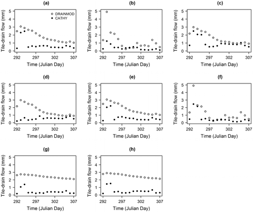
According to two values of PEP and PEV simulated by each model, it can be noted that their values were lower for scenario 3, and consequently the tile-drain flow hydrographs had very similar behaviour for this scenario. Therefore, the KsXY values of this scenario constituted the starting point of the calibration process for both models.

Calibration and validation

Calibration procedure – tile drain flow

Observed and simulated tile drain flow plots are reported in Figure 4, while statistics of model performance during the calibration periods (summer and fall 2011) are introduced in Table 7. Two different behaviours can be noticed. During summer, DRAINMOD and CATHY are on either side of the observed hydrographs, while in the fall DRAINMOD overestimates drained flow whereas CATHY underestimates drained flow.

Figure 4. DRAINMOD and CATHY predicted and observed tile-drain flow comparison during calibration process: (a) summer 2011 and (b) fall 2011.

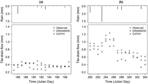
Table 7. Statistical comparison between simulated and observed tile-drain flow for the calibration periods. (TPDF: total predicted drain flow, TODF: total observed drain flow, R²: coefficient of determination, NSE: coefficient of efficiency (Nash), NSEm: modified coefficient of efficiency).

Period	Summer 2011		Fall 2011
TODF (mm)	5.85		11.52
Model	DRAINMOD	CATHY	DRAINMOD	CATHY
TPDF (mm)	5.66	5.28	12.88	10.18
TPDF/TODF (-)	0.98	0.90	1.12	0.88
R^2 (-)	0.36	0.02	0.96	0.76
NSE (-)	−0.50	−8.32	0.67	0.34
NSEm (-)	0.90	−0.32	0.99	0.96

Globally the two models yield low performance (low values of R² and NSE) during summer (0.36 and −0.50 for DRAINMOD, and 0.02 and −8.32 for CATHY). During the fall, DRAINMOD performed well (R² = 0.96; NSE = 0.67). Meanwhile, CATHY did not perform as well, with smaller values of R² (0.74) and NSE (0.34). In terms of total predicted drain flow (mm, TPDF) and total observed drain flow (mm, TODF), the two models performed well for both summer and fall 2011. According to these calibration results, both models had better statistical performance during the fall than in the summer, with larger values of TODF (11.52 mm versus 5.85 mm) and of TPDF (12.88 m versus 5.66 mm) for DRAINMOD and 10.18 mm versus 5.28 mm for CATHY.

Validation procedure – tile drain flow

The shape of predicted and observed drain flow plots during the validation periods (falls 2010 and 2012) are shown in Figure 5 and their performance metrics are summarized in Table 8. As mentioned before, CATHY and DRAINMOD curves are on either side of the observed curve during the first validation period, and during the second validation period DRAINMOD tends to overestimate while CATHY tends to underestimate the tile-drain flows.

Figure 5. DRAINMOD and CATHY predicted and observed tile-drain flow comparison during validation process: (a) fall 2010; and (b) fall 2012.

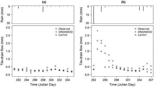
Table 8. Statistical comparison between simulated and observed tile-drain flow for the validation periods. (TPDF: total predicted drain flow, TODF: total observed drain flow, R²: coefficient of determination, NSE: coefficient of efficiency (Nash), NSEm: modified coefficient of efficiency).

Period	Fall 2010		Fall 2012
TODF (mm)	4.29		10.46
Model	DRAINMOD	CATHY	DRAINMOD	CATHY
TPDF (mm)	4.47	4.21	13.67	7.67
TPDF/TODF (-)	1.04	0.98	1.31	0.73
R^2 (-)	0.31	0.10	0.97	0.87
NSE (-)	−0.25	−1.41	0.79	0.73
NSEm (-)	0.61	0.22	0.95	0.92

The performance metrics indicate low performances for the two models during fall 2010 (R² = 0.31 and NSE = −0.25 for DRAINMOD: R² = 0.10 and NSE = −1.41 for CATHY); and excellent performance during fall 2012 (R² = 0.97 and NSE = 0.79 for DRAINMOD; R² = 0.87 and NSE = 0.73 for CATHY). For falls 2010 and 2012, the total tile-drain flows simulated by the models were good, with TODF values of 4.29 and 10.46 mm compared to TPDF values of 4.47 and 13.67 mm for DRAINMOD, and 4.21 and 7.67 mm for CATHY. Besides summer 2011, it is noteworthy that during all other calibration and validation periods, TPDF/TODF ratios for DRAINMOD are higher than 1.0 (1.12, 1.13 and 1.04 during falls 2010, 2011 and 2012, respectively) and those for CATHY are lower than 1.0 (0.88, 0.73 and 0.98 during falls 2010, 2011 and 2012, respectively), and their relative departures from 1.00 are almost the same. These results revealed good performances and illustrate that DRAINMOD over-predicted while CATHY under-predicted subsurface drainage flow.

Figure 6 illustrates the tile-drain flows predicted by DRAINMOD and CATHY, and the uncertainty range (in gray) associated with an error of ± 20% on observed drained flows for all simulation periods. The corresponding NSE_m (see Table 5 for definition) values are given in Tables 7 and 8. It was found that NSE_m increased the performance of the models compared to NSE. For example, the DRAINMOD simulated drained flows were practically within the uncertainty range, characterized by an NSE_m value closed to 1.00 for fall 2011. Larger NSE_m values for the two models were noted for falls 2011 and 2012, corresponding to larger observed tile-drain flows. Hence, CATHY performed very well (0.96 and 0.92 instead of 0.34 and 0.73 in terms of NSE). The two models were calibrated and validated using only observed tile drain flows. It is very important to note that under ideal conditions, water table elevation should be also used as a calibration criterion.

Figure 6. DRAINMOD and CATHY predicted tile-drain flows and the uncertainty range (in gray) with an error of ± 20% on observed tile-drain flows: (a) summer 2011; (b) fall 2011; (c) fall 2010; and (d) fall 2012.

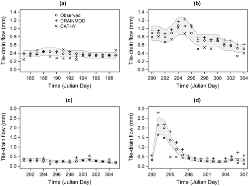
It is noteworthy that during an inter-comparison study of MIKE-SHE (spatially distributed, watershed-scale model) and DRAINMOD (lumped, field-scale model) in terms of their performance in predicting stream flow (as a sum of subsurface drainage and surface runoff), Dai et al. (2010) observed that both models showed relatively large uncertainty in simulating stream flow for dry years. Similarly, the results of this study show that the performances of DRAINMOD and CATHY were low during dry periods. Meanwhile, both models successfully simulated subsurface drainage during periods characterized by larger observed tile-drain flow values.

Potential evapotranspiration and actual evapotranspiration comparison

Figure 7 illustrates the time-dependent cumulative PET and model cumulative AET while Table 9 shows R² values for AET versus PET, and the difference between total potential evapotranspiration (TPET) and total actual evapotranspiration (TAET) over TPET (%). There was good corroboration between evapotranspiration estimates from the two models (R² > 0.80). Differences between PET and AET were greater for DRAINMOD than for CATHY based on the (TPET − TAET)/TPET values, which varied from 19.97 to 40.03% for DRAINMOD, and from 15.32 to 27.54% for CATHY. These results reveal the fact that during a day with precipitation, DRAINMOD considers evapotranspiration to be zero. Thus, its TAET at the end of the simulation period is lower than that of CATHY.

Figure 7. Cumulative PET and cumulative AET simulated by DRAINMOD and CATHY: (a) summer 2011; (b) fall 2011; (c) fall 2010; and (d) fall 2012. (PET: Potential Evapotranspiration, AET: Actual Evapotranspiration).

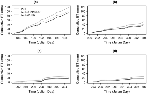
Table 9. Model performance in simulating actual evapotranspiration.

Criteria	R^2 (AET versus PET) (-)				(TPET-TAET)/TPET (%)
Model	S 2011	F 2011	F 2010	F 2012	S 2011	F 2011	F 2010	F 2012
DRAINMOD	0.84	0.94	0.97	0.95	19.97	25.54	40.03	38.73
CATHY	0.96	0.95	0.98	0.97	15.32	18.50	27.54	23.46

S: summer; F: fall, PET: Potential Evapotranspiration, AET: Actual Evapotranspiration, TPET: Total Potential Evapotranspiration, TAET: Total Actual Evapotranspiration.

Impact of saturated hydraulic conductivity

The one-at-a-time change in KsXY of each layer of the porous media had a differential effect on the tile-drain flow simulated by both models (Figure 8). Compared to the validation cumulative tile-drain flow scenario (VSc), the first layer (L1) and second layer (L2) generally did not have an effect on drained flow when multiplying or dividing KsXY by 10 for the two models. When KsXY was divided by 10 in the third and fourth layers (L3 and L4), tile-drain flow given by DRAINMOD and CATHY slightly increased and decreased in the first case, and decreased and increased in the second case, respectively. For DRAINMOD, it was noticed for VSc that the cumulative tile-drain flow increased with an increase in the L4 KsXY value (multiplied by 10) and that the cumulative tile-drain flow decreased when both L3 and L4 KsXY values increased. For CATHY, the tile-drain flow decreased when multiplying KsXY value by 10 in L3 and L4, but the tile-drain flow decrease induced by L4 was higher than that of L3.

Figure 8. Impact of lateral saturated hydraulic conductivity (KsXY) change in each layer (variation of value of layer 1 (L1), 2 (L2), 3 (L3), 4 (L4)) of the porous media one at a time with respect to the cumulative tile-drain flow: (a) 1/10 KsXY – DRAINMOD; (b) 10 KsXY – DRAINMOD; (c) 1/10 KsXY – CATHY; and (d) 10 KsXY – CATHY.

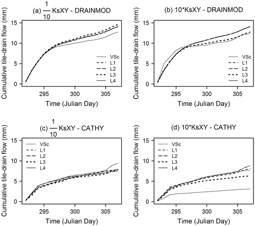
For CATHY, Muma et al. (2014) found that the most influential parameter with respect to tile-drain flow and stream flow from a micro-watershed was KsXY in layers underlying those in which the tile-drain systems are located. By multiplying or dividing KsXY by 10 in each layer at a time, the current study further highlights that layers below the subsurface drainage network had an important impact on tile-drain flow.

Conclusions

The capability of two models, DRAINMOD and CATHY, to simulate tile-drain flow was evaluated and compared. From a goodness-of-fit point of view, the results showed that the performance of the two models was low during low observed subsurface drainage flow. The model calibration and validation during periods with higher observed subsurface drainage revealed on the one hand that DRAINMOD tended to over-predict subsurface drainage discharge, while CATHY tended to under-predict flow. On the other hand, when looking at the total tile-drain flow ratios, both models performed well, with DRAINMOD yielding better results than CATHY. With respect to (computed) potential evapotranspiration, the two models had similar results. The differences between them are related to the processes simulated by each model, namely the exfiltration and seepage processes and evaporation on days with precipitation. According to the impact of horizontal saturated hydraulic conductivity on tile-drain flow, efforts should be focused on making additional measurements of the saturated hydraulic conductivity of the layers underlying the tile-drain system.

The validation of CATHY to simulate subsurface drainage will be further tested by installing an automatic tile-drain system for flow measurement at the field plot in order to obtain additional tile-drain flow data. This study could benefit from field measurements of evapotranspiration to further validate the simulated actual evapotranspiration. In order to analyze the performance of the models with respect to water table elevation, a piezometer should be installed in the center of the tile drain plot.

This study demonstrated that both DRAINMOD and CATHY can reliably predict subsurface drainage flow during wet periods, which is the time when it is imperative to know whether a tile-drain system can meet design criteria. On another front, this study illustrated that even if a model has been widely applied to design and understand artificial drainage systems (DRAINMOD), there can be field conditions under which the model cannot yield satisfactory results because of the misrepresentation of some main hydrological processes. Meanwhile, application of a more complex model (CATHY) does not necessarily imply increased simulation performance. Therefore, the use or application of a model depends on the nature of the problem or the modeling objectives.

Acknowledgements

The authors wish to thank Eric van Bochove, Georges Thériault, Catherine Bossé, Geneviève Montminy, Michel Nolin, Luc Lamontagne, and Mario Deschênes of Agriculture and Agri-food Canada for providing data. Special thanks to Brook Harker and David Kiely of AAC for their coordination of the WEBs (Watershed Evaluation of Beneficial Management Practices) project. This study has received financial support from AAC (A.N. Rousseau, principal investigator of the project “Hydrological-economic modelling of Beneficial Managements Practices impact on water quality in an agricultural watershed”) and Ontario Ministry of Agriculture, Food and Rural Affairs (OMAFRA; Wanhong Yang of the University of Guelph, principal investigator of the project “Evaluating the Cost Effectiveness of Multiple Best Management Practices in Agricultural Watersheds”).

References

- Allen, R. G., L. S. Pereira, D. Raes, and M. Smith. 1998. Crop evapotranspiration: Guidelines for computing crop water requirements. Irrigation and Drainage Paper 56, FAO, Roma.
- Bengtson, R. L., C. E. Carter, J. L. Fouss, L. M. Southwick, and G. H. Willis. 1995. Agricutural drainage and water quality in the Mississippi delta. Journal of Irrigation and Drainage Engineering 121 (4): 292–295.10.1061/(ASCE)0733-9437(1995)121:4(292)
- Bessiere, H. 2008. Variational data assimilation for distributed hydrological modeling of fast kinetic flood. Thèse de doctorat, Université de Toulouse, Institut National Polytechnique de Toulouse, 321.
- Bixio, A. C., S. Orlandini, C. Paniconi, and M. Putti. 2000. Physically-based distributed model for coupled surface runoff and subsurface flow simulation at the catchment scale. In Computational methods in water resources, eds. L. R. Bentley, J. F. Sykes, C. A. Brebbia, W. G. Gray, and G. F. Pinder, 2: 1115–1122. Rotterdam, The Netherlands: Balkema.
- Bouarfa, S., and D. Zimmer. 2000. Water-table shapes and drain flow rates in shallow drainage systems. Journal of Hydrology 235 (3–4): 264–275.10.1016/S0022-1694(00)00280-8
- Brunner, P., and C. T. Simmons. 2012. HydroGeoSphere: A fully integrated. Physically Based Hydrological Model. Ground Water 50 (2): 170–176.
- BTSAC (Basin Technical and Scientific Advisory Committee). 2012. Water management options for subsurface drainage: Briefing Paper 2. http://www.rrbdin.org/archives/4520 (accessed June 2014).
- Camporese, M., C. Paniconi, M. Putti, and S. Orlandini. 2010. Surface-subsurface flow modeling with path-based runoff routing, boundary condition-based coupling, and assimilation of multisource observation data. Water Resources Research 46 (2): W02512.
- Carlier, J. P., C. Kao, and I. Ginzburg. 2007. Field-scale modeling of subsurface tile-drained soils using an equivalent-medium approach. Journal of Hydrology 341 (1–2): 105–115.10.1016/j.jhydrol.2007.05.006
- Culley, J. L. B., and E. F. Bolton. 1983. Suspended solids and phosphorus loads from a clay soil: II. Watershed study. Journal of Environmental Quality 12 : 498–503.10.2134/jeq1983.00472425001200040012x
- Cuo, L., T. W. Giambelluca, A. D. Ziegler, and M. A. Nullet. 2006. Use of the distributed hydrology soil vegetation model to study road effects on hydrological processes in Pang Khum Experimental Watershed, northern Thailand. Forest Ecology and Management 224 (1–2): 81–94.10.1016/j.foreco.2005.12.009
- Cuo, L., D. P. Lettenmaier, M. Alberti, and J. E. Richey. 2009. Effects of a century of land cover and climate change on the hydrology of the Puget Sound basin. Hydrological Processes 23 (6): 907–933.10.1002/hyp.v23:6
- Cuo, L., T. W. Giambelluca, and A. D. Ziegler. 2011. Lumped parameter sensitivity analysis of a distributed hydrological model within tropical and temperate catchments. Hydrological Processes 25 (15): 2405–2421.10.1002/hyp.v25.15
- Dai, Z., D. M. Amatya, G. Sun, C. C. Trettin, and H. Li. 2010. A comparison of MIKE-SHE and DRAINMOD for modeling forested wetland hydrology in coastal South Carolina, USA. XVIIth World Congress of the International Commission of Agricultural Engineering (CIGR), Quebec City, Canada, June 13–17.
- DHI. 2007. MIKE-SHE user manual, volume 2: Reference guide. Danemark: DHI Water and Environment, Danish Hydraulic Institute.
- Dolezal, F., Z. Kulhavy, M. Soukup, and R. Kodesova. 2001. Hydrology of tile drainage runoff. Physics and Chemistry of the Earth, Part B: Hydrology, Ocean and Atmosphere 26 (7–8): 623–627.10.1016/S1464-1909(01)00059-4
- Dunn, S. M., and R. Mackay. 1996. Modelling the hydrological impact of open ditch drainage. Journal of Hydrology 179 (1–4): 37–66.10.1016/0022-1694(95)02871-4
- Eggelsmann, R. 1981. Drainage management for farming, civil engineering and lanscaping. 2nd ed. Hamburg, Berlin: Verlag Paul Parey.
- Ernst, L. F. 1962. Groundwater movement in the saturated zone and calculation in the presence of horizontal parallel open channels. Versl. Landbouwk. Onderz. 67.15. Wageningen: PUDOC, 189.
- Fipps, G., and R. Skaggs. 1991. Simple methods for predicting flow to drains. Journal of Irrigation and Drainage Engineering 117 (6): 881–896.10.1061/(ASCE)0733-9437(1991)117:6(881)
- Fipps, G., R. W. Skaggs, and J. L. Nieber. 1986. Drains as a boundary condition in finite elements. Water Resources Research 22 (11): 1613–1621.10.1029/WR022i011p01613
- Gadd, N. R. 1974. Surficial geology - Saint-Sylvestre. Geological Survey of Canada, Ottawa, ( 1:50000).
- van Genuchten, M. T., and D. R. Nielsen. 1985. On describing and predicting the hydraulic properties of unsaturated soils. Annales Geophysicae 3 (5): 615–628.
- Holden, J., P. J. Chapman, and J. C. Labadz. 2004. Artificial drainage of peatlands: hydrological andhydrochemical process and wetland restoration. Progress in Physical Geography 28 (1): 95–123.10.1191/0309133304pp403ra
- Hooghoudt, S. 1940. Hooghoudt’s theory of drainage. Technical report. The Netherlands: Institut voor Cultuurtechnik en Waterhuishouding (in Dutch).
- Istok, J. D., and G. F. Kling. 1983. Effect of subsurface drainage on runoff and sediment yield from an agricultural watershed in western Oregon, USA. Journal of Hydrology 65 (4): 279–291.10.1016/0022-1694(83)90082-3
- King, K. W., N. R. Fausey, and M. R. Williams. 2014. Effect of subsurface drainage on streamflow in an agricultural headwater watershed. Journal of Hydrology 519 (Part A): 438–445.10.1016/j.jhydrol.2014.07.035
- King, K. W., M. R. Williams, and N. R. Fausey. 2015. Contributions of systematic tile drainage to watershed-scale phosphorus transport. Journal Environmental Quality 44 (2): 486–494.10.2134/jeq2014.04.0149
- Kirkham, D. 1958. Seepage of steady rainfall through soil into drains. Transactions of American Geophysical Union 39 (5): 892–908.10.1029/TR039i005p00892
- Kleinman, P. J. A., D. R. Smith, C. H. Bolster, and Z. M. Easton. 2015. Phosphorus fate, management, and modeling in artificially drained systems. Journal Environmental Quality 44 (2): 460–466.10.2134/jeq2015.02.0090
- Kroes, V. D., P. Groenendijk, R. F. A. Hendriks, and C. M. J. Jacobs. 2008. SWAP version 3.2 theory description and user manual, Alterrareport, Wageningen, 262.
- Kung, K. J. S., E. J. Kladivko, T. J. Gish, T. S. Steenhuis, G. Bubenzer, and C. S. Helling. 2000. Quantifying preferential flow by breakthrough of sequentially applied tracers: Silt loam soil. Soil Science Society of America Journal 64 (4): 1296–1304.10.2136/sssaj2000.6441296x
- Lamontagne, L., A. Martin, and M. C. Nolin. 2010. A pedological study of the Bras d'Henri watershed (Quebec). Québec: Laboratoires de pédologie et d’agriculture de précision, Centre de recherche et de développement sur les sols et les grandes cultures, Service national d’information sur les terres et les eaux, Direction générale de la recherche, Agriculture et Agroalimentaire Canada.
- Larsbo, M., and N. Jarvis. 2003. MACRO 5.0. A model of water flow and solute transport in macroporous soil. Technical description, Swedish University of Agricultural Sciences, 40.
- MacQuarrie, K. T. B., and E. A. Sudicky. 1996. On the incorporation of drains into three-dimensional variably saturated groundwater flow models. Water Resources Research 32 (2): 477–482.10.1029/95WR03404
- Macrae, M. L., M. C. English, S. L. Schiff, and M. Stone. 2007. Intra-annual variability in the contribution of tile drains to basin discharge and phosphorus export in a first-order agricultural catchment. Agricultural Water Management 92 (3): 171–182.10.1016/j.agwat.2007.05.015
- Magner, J. A., G. A. Payne, and L. J. Steffen. 2004. Drainage effects on stream nitrate-n and hydrology in South-Central Minnesota (USA). Environmental Monitoring Assessment 91 (1–3): 183–198.10.1023/B:EMAS.0000009235.50413.42
- Moradkhani, H., and S. Sorooshian. 2008. General review of rainfall-runoff modeling: Model calibration, data assimilation, and uncertainty analysis. Hydrological modeling and the water cycle.Springer. 291 p. ISBN 978-3-540-77842-4.
- Muma, M., S. J. Gumiere, and A. N. Rousseau. 2014. Comprehensive analysis of the CATHY model sensitivity to soil hydrodynamic properties of a tile-drained agricultural micro-watershed. Hydrological Sciences Journal 59 (8): 1606–1623.10.1080/02626667.2013.843778
- Oudin, L. 2004. Research of a relevant evapotranspiration model as an input of a global rainfall-runoff model. Thèse de doctorat, École Nationale de Génie Rural, des Eaux et Forets, Paris, France, 495.
- Pereira, L. S., R. G. Allen, and A. Perrier. 2006. Practical method of calculating water requirements. 2e ed., eds. J. R. Tiercelin, and A. Vidal, 227–268. Paris: Lavoisier.
- Robinson, M. 1990. Impact of improved land drainage on river flows. Institute of Hydrology Report no. 113. Center for Ecology and Hydrology, Edinburgh, UK.
- Robinson, M., and D. W. Rycroft. 1999. The impact of drainage on stream flows. Agronomy Monograph 38 : 767–800.
- Schilling, K. E., and M. Helmers. 2008. Effects of subsurface drainage tiles on streamflow in Iowa agricultural watersheds: Exploratory hydrograph analysis. Hydrological Processes 22 (23): 4497–4506.10.1002/hyp.v22:23
- Serrano, S. E., H. R. Whiteley, and R. W. Irwin. 1985. Effects of agricultural drainage on streamflow in the Middle Thames River, Ontario, 1949–1980. Canadian Journal of Civil Engineering 12 (4): 875–885.10.1139/l85-100
- Šimůnek, J., K. Huang, and M. Th. van Genuchten. 1995. The SWMS_3D code for simulating water flow and solute transport in three-dimensional variably-saturated media. Riverside, CA: U.S. Salinity Laboratory Agricultural Research Service, U.S. Department of Agriculture, 155.
- Skaggs, R. W. 1978. A water management model for shallow water table soils. Technical Report n°134. Water Resources Research Institute, North Carolina State University, Raleigh
- Skaggs, R. W. 1980. DRAINMOD: Reference report. http://www.bae.ncsu.edu/soil_water/documents/drainmod/chapter1.pdf (Accessed June 2014).
- Skaggs, R. W., M. A. Breve, and J. W. Gilliam. 1994. Hydrologic and water quality impacts of agricultural drainage. Critical Reviews in Environmental Science and Technology 24 (1): 1–32.10.1080/10643389409388459
- Skaggs, R. W., M. A. Youssef, and G. M. Chescheir. 2012. DRAINMOD: Model use, calibration, and validation. Transactions of the ASABE 55 (4): 1509–1522.10.13031/2013.42259
- Smith, D. R., K. W. King, L. Johnson, W. Francesconi, P. Richards, D. Baker, and A. N. Sharpley. 2015. Surface runoff and tile drainage transport of phosphorus in the Midwestern United States. Journal of Environmental Quality 44 (2): 495–502.10.2134/jeq2014.04.0176
- St-Hilaire, A., S. Duchesne, and A. N. Rousseau. 2015. Floods and water quality in Canada – A review of the interactions with urbanization, agriculture and forestry. Canadian Water Resources Journal 41 (1–2): 273–287. doi:10.1080/07011784.2015.1010181.
- Therrien, R., R. G. McLaren, E. A. Sudicky, and S. M. Panday. 2007. HydroGeo-Sphere: A three-dimensional numerical model describing fully-integrated subsurface and surface flow and solute transport: User manual. Groundwater Simulation Group. Waterloo, ON, Canada: University of Waterloo.
- Thornthwaite, C. W. 1948. An Approach toward a rational classification of climate. Geographical Review 38 (1): 55–94.10.2307/210739
- Tomer, M. D., D. W. Meek, and L. A. Kramer. 2005. Agricultural practices influence flow regimes of headwater streams in Western Iowa. Journal Environmental Quality 34 (5): 1547–1558.10.2134/jeq2004.0199
- Vidon, P., and P. E. Cuadra. 2011. Phosphorus dynamics in tile-drain flow during storms in the US Midwest. Agricultural Water Management 98 (4): 532–540.10.1016/j.agwat.2010.09.010
- Walter, I. A., R. G. Allen, R. Elliot, M. E. Jensen, D. Itenfisu, B. Mechan, T. A. Howell, et al. 2005. The ASCE standardized reference evapotranspiration equation. http://www.kimberly.uidaho.edu/water/asceewri/ascestzdetmain2005.pdf (Accessed June 2014).
- Xue, Y., M. B. David, L. E. Gentry, and D. A. Kovacic. 1998. Kinetics and modeling of dissolved phosphorus export from a tile-drained agricultural watershed. Journal Environmental Quality 27 (4): 917–922.10.2134/jeq1998.00472425002700040028x
- Yang, W., A. N. Rousseau, and P. Boxall. 2007. An integrated economic-hydrologic modeling framework for the watershed evaluation of beneficial management practices. Journal of Soil and Water Conservation 62 (6): 423–432.
- Zucker, L. A., and L. C. E.Brown, eds. 1998. Agricultural drainage: Water quality impacts and subsurface drainage studies in the Midwest. Ohio State University Extension Bulletin 871. The Ohio State University.