Pixel-Based Image Compositing for Large-Area Dense Time Series Applications and Science

Abstract

Free and open access to the more than 40 years of data captured in the Landsat archive, combined with improvements in standardized image products and increasing computer processing and storage capabilities, have enabled the production of large-area, cloud-free, surface reflectance pixel-based image composites. Best-available-pixel (BAP) composites represent a new paradigm in remote sensing that is no longer reliant on scene-based analysis. A time series of these BAP image composites affords novel opportunities to generate information products characterizing land cover, land cover change, and forest structural attributes in a manner that is dynamic, transparent, systematic, repeatable, and spatially exhaustive. Herein, we articulate the information needs associated with forest ecosystem science and monitoring in a Canadian context, and indicate how these new image compositing approaches and subsequent derived products can enable us to address these needs. We highlight some of the issues and opportunities associated with an image compositing approach and demonstrate annual composite products at a national-scale for a single year, with more detailed analyses for two prototype areas using 15 years of Landsat data. Recommendations concerning how to best link compositing decisions to the desired use of the composite (and the information need) are presented, along with future research directions.

Résumé

L’accès libre et gratuit à plus de 40 ans de données dans l’archive Landsat combiné à l’amélioration des produits d’imagerie standardisés et l’augmentation des capacités de traitement et de stockage informatiques ont permis la production d’images composites basées sur les pixels de réflectance de surface de grande superficie sans nuages. Les composites du « meilleur pixel disponible » (best-available-pixel; BAP) représentent un nouveau paradigme en matière de télédétection qui ne dépend plus de l’analyse par scène. Une série chronologique de ces images composites BAP offre de nouvelles occasions de générer des produits d’information qui caractérisent la couverture terrestre, le changement de la couverture terrestre et les attributs structurels de la forêt d’une manière dynamique, transparente, systématique, répétable et spatialement exhaustive. Ici, nous articulons les besoins d’information liés à la science et à la surveillance des écosystèmes forestiers dans un contexte canadien, et nous indiquons comment ces nouvelles approches de composition d’image et les produits qui en découlent peuvent nous permettre de répondre à ces besoins. Nous soulignons quelques-uns des problèmes et des possibilités associés à une approche de composition d’image et nous démontrons des produits composites annuels à l’échelle nationale pour une année, avec des analyses plus détaillées pour deux zones prototypes utilisant 15 ans de données Landsat. Des recommandations concernant la meilleure façon de lier des décisions de composition d’images à l’utilisation souhaitée du composite (et le besoin d’information) ainsi que les orientations futures de la recherche sont présentées.

INTRODUCTION

Free and open access to the Landsat archive enables the generation of pixel-based composites that can be used to address a broad range of information needs associated with national ecosystem monitoring. For a country the size of Canada (approaching 10 million km²), with limited access to remote forests and a multiplicity of jurisdictions responsible for resource stewardship, remotely sensed data offers the only viable means, economic or otherwise, to generate national information products for ecosystem monitoring in a dynamic, transparent, systematic, repeatable, and spatially exhaustive manner (Wulder et al. 2007a; Falkowski et al. 2009). Landsat data brings two key elements to ecosystem monitoring: a spatial dimension that is at a scale appropriate for capturing anthropogenic impacts (Townshend and Justice 1988), and a temporal dimension that enables retrospective analyses and characterization of changes over the more than 40 years of data captured by successive Landsat sensors (Wulder et al. 2012). Pixel-based image compositing with Landsat is a new paradigm in remote sensing science that applies a suite of user-defined rules to leverage the extensive Landsat archive for generating cloud-free, radiometrically and phenologically consistent image composites that are spatially contiguous over large areas (Roy et al. 2010; Hansen and Loveland 2012; Griffiths et al. 2013).

Pixel-based image compositing of Landsat data has emerged from a unique confluence of scientific and operational developments, predicated by free and open access to the Landsat archive (Woodcock et al. 2008; Wulder et al. 2012), and supported by the computing and data storage capacity to fully automate radiometric and geometric pre-processing and create increasingly robust standardized image products (Masek et al. 2006; Roy et al. 2010). Prior to the era of free access to the Landsat archive, pixel-based compositing approaches were limited to low spatial resolution data, with pixels 500 × 500 m or greater, such as Advanced Very High Resolution Radiometer (AVHRR) (Holben 1986; Cihlar et al. 1994) and MODerate-resolution Imaging Spectrometer (MODIS) (Roy 2000; Justice et al. 2002; Ju et al. 2010). Common to these datasets is their free availability with near-daily global coverage allowing for selection of pixels based upon user-defined rules. The compositing approaches were used primarily to reduce the impact of clouds, aerosol contamination, and view angle effects, as well as data volumes (Holben 1986; Cihlar et al. 1994). Due to the large number of observations available, AVHRR and MODIS compositing approaches were relatively simple, using rules such as the maximum Normalized Difference Vegetation Index (NDVI) or the minimum view angle to select the “best” observation for a given pixel within a specified compositing period (e.g., 16 days) (Wolfe et al. 1998). For Landsat, high data purchase costs prior to 2008 precluded the application of any such data-intensive compositing approach. With the opening of the Landsat archive, compositing approaches using Landsat data became economically feasible. Such approaches have benefitted and been informed by earlier compositing methods developed for AVHRR and MODIS data (Roy et al. 2010).

Early efforts at compositing with Landsat serendipitously took advantage of the overlap between adjacent Landsat scenes. For example, Du et al. (2001) created a large-area Landsat mosaic and applied pixel-based compositing in overlap areas between adjacent scenes, selecting the pixel with the highest NDVI for the final composite. Post-classification compositing of Landsat data from scene overlap areas has also been used to produce large-area land cover products (Guindon and Edmonds 2002; Wijedasa et al. 2012). Epochal global Landsat datasets—whereby single best observations are selected over a given time period—were also produced and distributed free of charge to the science community and the general public via the Global Land Survey (GLS) project (Townshend et al. 2012; Gutman et al. 2013). The 1975, 1990, and 2000 GLS datasets were produced using the best single-date image for each Landsat path/row (Tucker et al. 2004), whilst the 2005 and 2010 GLS data were produced via compositing up to three dates of imagery for each path/row, primarily to fill gaps resulting from Scan Line Corrector (SLC)-off data (Gutman et al. 2013). Given the limited availability of cloud-free Landsat data in some areas of the globe, epochal composites have been used extensively to support change detection studies (e.g., Hansen et al. 2008; Potapov et al. 2011). Lindquist et al. (2008) evaluated the potential of the epochal 2000 and 2005 GLS datasets, relative to more data intensive per-pixel compositing approaches (e.g., Hansen et al. 2008), for mapping forest cover change in the tropics. The authors concluded that in order to provide sufficient spatial coverage to support change detection between epochs, Landsat-based image compositing approaches should make use of all available Landsat data for any given path/row (and certainly more than the three images prescribed for in the GLS products). In a similar study, Broich et al. (2011) generated epochal Landsat composites for 2000 and 2005 over Sumatra and Kalimantan, Indonesia and assessed the efficacy of these composites for quantifying forest cover change. The authors found that a time series approach that used “all good land observations” provided more accurate estimates of forest cover change when compared to change maps generated from the epochal composites. It should be noted however that these epochal composites were generated to serve a broad range of applications and were not tailored specifically to forest monitoring.

Since the opening of the Landsat archive in 2008, several Landsat compositing approaches have emerged in the literature (Table 1). Many of the approaches have relied exclusively on Landsat Enhanced Thematic Mapper (ETM+ data) corrected to TOA reflectance (Roy et al. 2010; Potapov et al. 2011, 2012). The per-pixel compositing approach applied by Hansen et al. (2008) that was later adapted by Potapov et al. (2011), relied on a MODIS-generated forest/non-forest mask to support radiometric normalization via a dark object subtraction (DOS) method (Chavez 1988). Potapov et al. (2012) further refined this approach, using a 10-year MODIS surface reflectance composite to facilitate band-wise mean bias adjustments with corresponding Landsat bands. For very large areas, the use of coarser spatial resolution data for normalization increases computational overhead and imposes temporal limitations related to the operational lifetime of a given satellite or sensor (i.e., precludes applicability to the pre-MODIS era in this case). A more recent trend is to combine observations from both TM and ETM+ that have been corrected to surface reflectance (Flood 2012; Griffiths et al. 2013) using standardized and largely automated approaches such as LEDAPS (Masek et al. 2006; Feng et al. 2013). Indeed, the United States Geological Survey (USGS) now provides Landsat surface reflectance products as a Climate Data Record (CDR)¹, and the provision of these higher level products could further reduce the amount of pre-processing required to enable pixel-based compositing in the same way that the standard Level-1 Terrain Corrected (L1T) products have enabled processing efficiencies (Hansen and Loveland 2012). L1T products are 8-bit with a compressed file size of approximately 250 MB/file (Landsat-8 L1T files are 16-bit with a compressed file size of 1GB/file). By contrast, CDR products are 16-bit, with a file size of approximately 500 MB/file. Given the increased file size of the CDR, there is a trade-off between downloading the larger CDR files via the internet, versus downloading the smaller L1T files and running LEDAPS locally to generate surface reflectance products.

TABLE 1 Review of studies applying Landsat pixel-based image compositing approaches

Study	Sensor	Physical Unit	Processing	# of unique path/row s	# of images	Compositing period	Cloud-masking	Rule-base
Hansen et al. 2008	TM, ETM+	TOA reflectance	MODIS forest/non-forest mask used as reference for normalization via dark object subtraction (DOS) and a regression-based surface anisotropic correction.	20	∼4–7 per path/row (98 total)	Two epochs: pre-1996 and post-1996	Custom (supervised classification using decision trees)	Selected image date with the lowest cloud and shadow likelihood; if two were equal used the pixel value closest to the forest reference value (TOA = 100).
Roy et al. 2010	ETM+	TOA reflectance	Standard practice for TOA estimation (Chander et al. 2009).	459	6521	Monthly, seasonal, annual (Dec 2007 to Nov 2008)	Custom (ACCA and supervised classification using decision trees)	Valid surface observations with minimal cloud, snow, and atmospheric contamination. Heritage maximum NDVI for vegetated pixels; maximum brightness temperature for unvegetated pixels; cloud masks.
Potapov et al. 2011	ETM+	TOA reflectance	MODIS forest/non-forest mask used as reference for normalization via DOS and regression-based surface anisotropic correction	406	7227	Two epochs: 2000 and 2005	Custom (supervised classification using CART decision trees)	Per-pixel QA assessment based on criteria for cloud/shadow and image date (year and season), then for probability of water and “no data”. QA assessment provided a data pool for selecting “best” observation. All data pool observations for each pixel were then ranked based on NIR values (band 4). The observation with a band 4 value closest to the pixel's band 4 median was selected for compositing.
Potapov et al. 2012	ETM+	TOA reflectance	Standard practice for TOA estimation (Chander et al. 2009). Normalized to MODIS 10-year surface reflectance using band-wise mean bias. Regression-based surface anisotropic correction.	120	8881	Two epochs: 2000–2005 and 2005–2010	Custom (supervised classification using CART decision trees)	As per Potapov et al. (2011) and described above.
Flood 2013	TM, ETM+	Surface reflectance	Atmospheric BRDF Topographic	1	Not reported. March 2000 to November 2012, minimum of 3 images per season	Seasonal composites (spring, summer, autumn, winter)	Fmask (Zhu and Woodcock 2012)	Medoid NDVI as a seasonally representative value
Griffiths et al. 2013	TM, ETM+	Surface reflectance	LEDAPS	42	Y2000 = 890; Y2005 = 1478; Y2010 = 1590	Three epochs: 2000, 2005, 2010.	Fmask (Zhu and Woodcock 2012)	Weighted pixel-based scoring system based on acquisition year, acquisition day of year, and distance of a given pixel to cloud.

The majority of compositing approaches detailed in Table 1 have relied on customized cloud detection algorithms, developed using supervised approaches such as decision tree classifiers (Hansen et al. 2008; Roy et al. 2010; Potapov et al. 2011, 2012). As an alternate, a robust automated cloud detection algorithm is now available that is being included into workflows for compositing approaches (i.e., Fmask; Zhu and Woodcock 2012). It should be noted that Fmask is also now being used in the production of CDR products (United States Geological Survey 2013).

Hansen and Loveland (2012) posit that advances in pixel-based image compositing signal the end of scene-based analysis approaches, making way for progressively more novel opportunities for large-area characterization and monitoring. This shift from a scene-based perspective to a pixel-based perspective for image understanding and processing is key, and certainly mirrors trends and developments in time series analysis approaches (Kennedy et al. 2010). The full impact of this change from scene-based to pixel-based analysis has yet to be realized. New approaches of providing data to users based upon multiple spatial and temporal considerations, rather than solely on image temporal resolution and programmatic acquisition plans are anticipated (e.g., area of interest driven rather than by path / row). Further, a best-available pixel philosophy also creates opportunities for fusion of multiple streams of image data from complementary sensors. For instance, given a sufficient level of similarity between image data and processing levels, the best-available pixels could come from different sensors. The Landsat series of sensors, with similar viewing geometry, precise geolocation, analogous band passes, and—critically—rigorous calibration that enables reflectance conversion, have offered insights into how measures from multiple satellites can be combined. The ability to integrate measures from different satellite programs in a virtual constellation would reduce reliance on individual satellite programs and offer an increased temporal resolution. The scheduled 2015 launch of Sentinel-2 will provide measures that are analogous to those of the Landsat-8 Operational Land Imager (OLI) and will provide an opportunity to develop and test a virtual constellation. Sentinel-2 is designed to place two satellites in orbit. A five day revisit will be realized with the launch of the second Sentinel-2 satellite (Drusch et al. 2012) and when combined with Landsat-8, a three day revisit cycle is anticipated. Areas of persistent cloud, such as some locations in the humid tropics, will remain a challenge for both Landsat and Sentinel, and although the increased revisit frequency increases the total number of acquisitions, it does not guarantee cloud-free observations (Kovalskyy and Roy 2013). Both Landsat-8 OLI and Sentinel-2 are calibrated instruments, allowing for conversion of at-satellite digital numbers to surface reflectance. Data blending techniques (such as those after Gao et al. 2006) also provide for the production of image values that could be included in a compositing application. Based upon the maturity of compositing algorithms and a growing suite of satellites and sources of suitable imagery, operational programs built upon these data streams are increasingly possible and appear sustainable.

There are a wide range of information needs that drive national mapping and change detection efforts in Canada that provide the motivation for transparent and operational image compositing applications. The objective of this paper is to present the context and current status of data and processing knowledge that allow for these needs to be met in a novel fashion through pixel-based image composites. We outline various approaches and considerations when developing pixel-based composites over large areas and define a lexicon that describes the different types of composites that may be generated and link these back to the required information needs. To demonstrate pixel-based compositing over large areas, we present an annual BAP composite for Canada for the year 2010. Then, to further demonstrate the potential for products to support times-series applications, we present 15 years of Landsat data from 1998 to 2012 for the province of Saskatchewan and the island of Newfoundland. We close with an exploration of potential applications and product directions and identify persistent issues and research opportunities that remain.

TABLE 2 Key attributes for Canada's NFI and Carbon Accounting programs

Attributes
Land cover
Crown closure
Age
Species
Height
Volume
Biomass
Pre-disturbance land cover
Post-disturbance land cover
Disturbance agent
Disturbance year
Disturbance extent (area)
Disturbance intensity

TABLE 3 A lexicon of pixel-based image composites

Composite type	Typical compositing period	Typical rule-base
Annual BAP	Target DOY ± 30 days (for a single year)	1. DOY (relative to a target DOY, i.e., Aug 1)
		2. Distance to cloud and cloud shadow
		3. Sensor
		4. Atmospheric opacity
Multi-year BAP	For a given target year and target DOY ± 30 days (± 1 or 2 years)	1. Year (relative to a target year)
		2. DOY (relative to a target DOY, i.e., Aug 1)
		3. Distance to cloud and cloud shadow
		4. Sensor
		5. Atmospheric opacity
Proxy value composite	Same as per annual BAP	Annual BAP composite used as source (generated using contextual rule-base as described above. Areas of no data or anomolous values are assigned a proxy value by examining a temporal trajectory of pixel values at the same or neightbouring pixel locations.

BACKGROUND

Forest Ecosystem Monitoring in Canada: Information Needs

In Canada, national forest data are needed to support a range of science and program information needs, policy development, and to fulfill national and international reporting obligations. For example, Canada produces an annual State of the Forest report (Natural Resources Canada 2013), and reports on specific criteria and indicators for sustainable forest management (Canadian Council of Forest Ministers 1995) and forest certification. Internationally, Canada has reporting commitments associated with the United Nations FAO Forest Resource Assessment program, The Montreal Process (Criteria and Indicators for the Conservation and Sustainable Management of Temperate and Boreal Forests), the United Nations Framework Convention on Climate Change, and the United Nations Convention on Biological Diversity. These data must be timely, consistent, and spatially exhaustive, and must enable assessment of trends over time, as well as characterization of non-timber resources (Gillis 2001). Canada's National Forest Inventory (NFI) is designed to provide the necessary data to support, in part, the aforementioned information needs; however, the NFI is a sample-based inventory, designed to survey a minimum of 1% of Canada's landmass (Gillis et al. 2005). There is a need to extend this information beyond the existing sample plots to provide spatially explicit information that can support increasingly sophisticated information and modelling requirements for both the NFI and carbon accounting programs, particularly for Canada's northern forest areas where there is currently the greatest paucity of forest information (Wulder et al. 2004; Falkowski et al. 2009). The attributes listed in Table 2 represent a subset of the full suite of attributes required by the NFI and carbon accounting programs (Gillis et al. 2005; Wulder et al. 2004; Kurz et al. 2009). This subset includes those attributes that are fundamental for meeting programmatic information needs. For example, land cover, crown closure, and height are necessary for the NFI to distinguish “forest” from “other wooded land”—an important distinction for reporting purposes (Gillis 2005). Some of the attributes presented in Table 2 are readily obtained from remotely sensed data (e.g., land cover, crown closure, and disturbance related attributes), whilst in other cases, remotely sensed data can be used to generate a proxy for the attribute of interest (i.e., time since disturbance as a proxy for age (Helmer et al. 2010)). Other attributes can be modeled (i.e. height, volume, and biomass), with the aid of an appropriate source of calibration data (e.g., Chen et al. 2012; Wulder et al. 2012). Of the items listed in Table 2, species is the most difficult attribute to determine using medium resolution remotely sensed data such as Landsat (e.g. van Aardt and Wynne (2001)), although forest types (e.g., coniferous, deciduous) can be reliably mapped (Wulder et al. 2007b).

FIG. 1. An overview of pixel-based image compositing methods used to generate prototype products for Saskatchewan and Newfoundland.

A Lexicon for Pixel-Based Image composites

In overall terms, we propose three unique types of pixel-based image composites: annual (single-year) composites, multi-year composites, and proxy-value composites (Table 3). Annual composites are surface reflectance composites that use the best available pixel observation (from the target year) for any given pixel location. Annual composites are produced using a set of specified rules that are defined according to the information need. For example, an annual composite may be designed to capture a specific time period or a limited phenological window (e.g., August 1 ± 30 days). In addition to a day-of-year rule, rules may also constrain observations according to sensor (e.g., preference for Landsat-5 over Landsat-7), distance to cloud and cloud shadows, and atmospheric opacity (to reduce the impact of haze). If there are no observations that satisfy the compositing rules for a given pixel location, then the pixel is coded as “no data” and as a result, annual composites may have areas of missing data. Multi-year composites are generated according to a set of user-specified rules; however, pixel observations from previous or subsequent years may be used when no suitable observation is found within a desired target year. Proxy value composites are annual BAP composites where “no data” pixels are populated using a time series of annual BAP composites to determine proxy values. Likewise, pixels with anomalous values—those that exceed a pre-defined range of expectation or which have opacity values indicative of hazy imagery—may also be assigned a proxy value. In essence, the objective of the proxy value composite is to assign the most similar value in time and space to a pixel that either has “no data” or has an anomalous value. Ideally, a pixel's full temporal trajectory is used to determine whether the pixel is stable over time (i.e., within an expected range of spectral values), or whether spectral change has occurred beyond a specified range of expectation. If a pixel has a stable trajectory, the infilling of missing values or resetting of anomalous values through the averaging (or some other method) of pixel values in the pixel's trajectory is possible. If the pixel's value is not stable through time, proxy values will have to be determined in accordance with spectral change events and (possibly) by examining the pixel's immediate spatial neighbourhood in the year of missing data. Detection of change events in the pixel's spectral trajectory is a necessary precursor to the generation of proxy value composites.

METHODS

An overview of the pixel-based imaging composite methods used to develop annual BAP composites is provided in Figure 1; details follow in the subsequent sections.

Study Area

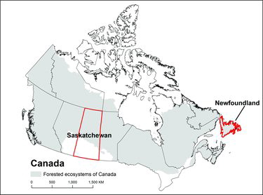
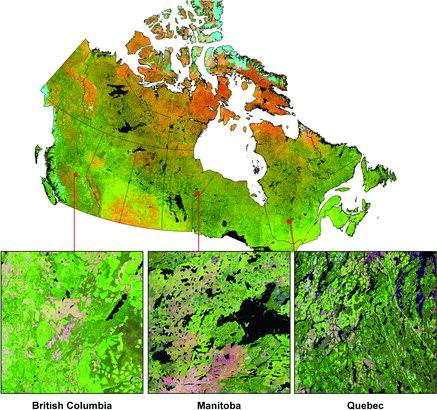
Approaching 10 million km² in area, Canada is a large nation with a gradient in ecosystem productivity that is influenced by latitude and precipitation (Hofgaard et al. 1999) (Figure 2). Forested ecosystems represent over 60% of Canada's land area (Wulder et al. 2008) and ninety-three percent of Canada's forests are publicly owned (Wulder et al. 2007a), with the capacity to harvest and process timber allocated through tenure agreements to the private sector (Haley and Luckert 1990). As a complex mosaic of trees, wetlands, and lakes, the forests of Canada represent 10% of global forests, and offer a range of ecosystem services that are economic, ecological, and sociocultural in nature. Canada's terrestrial area is represented by 1285 unique WRS-2 path/rows and approximately 10.7 billion 30 x 30 m pixels. Saskatchewan is the seventh largest province or territory in Canada with an area of approximately 651,900 km². More than half of this area is forest, with wildfire as the dominant disturbance agent (Saskatchewan Ministry of Environment 2012). Saskatchewan is comprised of approximately 702 million 30 × 30 m pixels (with 71 WRS-2 path/row locations), and has a diverse forest assemblage and a latitudinal gradient. Newfoundland has an area of approximately 108,860 km² with 46% of this area considered forest (Department of Forest Resources and Agrifoods 2003). Newfoundland is the most eastern extent of the Boreal Shield Ecozone and its forests are typically composed of small trees that are primarily coniferous species, with the dominant species being Black spruce (Picea mariana [Mill.] B.S.P.). Newfoundland is an island and is comprised of approximately 122 million 30 × 30 m pixels (with 21 WRS-2 path/row locations).

FIG. 2. Study area: Canada, Saskatchewan, and Newfoundland.

Data

Candidate images for producing an annual composite for a given year were selected from the Landsat metadata archive based on distance to a specified target day of year (DOY) and percent cloud cover. Images acquired within ±62 days of the target DOY with less than 70% cloud cover were considered viable candidates for compositing. A target DOY of August 1 (Julian day 213) was selected for its likelihood of being within the growing season for the majority of Canada's terrestrial landscape (McKenney et al. 2006). In Canada's north (that is, >60°N) the date range for candidate images was further restricted to ±30 days, to minimize the presence of snow cover. Image overlap is significant in the north (i.e. 85% at 80°N; Wulder and Seemann 2001) increasing the likelihood of cloud-free observations despite the more limited date range for candidate images. When cloud cover exceeds 70%, images are difficult to geometrically correct due to obscured ground control points (White and Wulder 2013). Identified candidate images were downloaded from the USGS Landsat archive as L1T products; L1T products are systematically corrected for radiometric, geometric, and terrain distortions (Irons et al. 2012). A master list of all candidate images for the area of interest is compiled that contains a user-generated unique numeric identifier for each image, as well as the unique Landsat scene identifier (i.e., LT50350232001211PC00). This list is used as a look-up table (LUT) to track the source image that is used for each pixel in order to support the development of image composites.

Pre-Processing

The L1T candidate images are pre-processed using Fmask (version 2.1), an object-based algorithm designed to identify clouds and cloud shadows, as well as clear land and water pixels, snow, and areas of no data (Zhu and Woodcock 2012). The Landsat Ecosystem Disturbance Adaptive System (LEDAPS; version 1.3.0; Schmidt et al. 2013) is used to generate surface reflectance values for use in the final image composite. LEDAPS produces top-of-atmosphere (TOA) reflectance from Landsat TM and ETM+ digital numbers (DN) and applies atmospheric corrections to generate a surface reflectance product (Masek et al. 2006). LEDAPS atmospheric corrections are based on the Second Simulation of a Satellite Signal in the Solar Spectrum (6S) radiative transfer model (Vermote et al. 1997).

Calculate Pixel Scores

Four scores were calculated for each pixel: sensor score, day of year score, distance to cloud or cloud shadow score, and opacity score. The sensor and DOY score were calculated at the image level (i.e., all pixels within the image receive the same score), whilst the cloud/cloud shadow and opacity scores were unique to each pixel. All scores were then summed to provide a total score for each pixel, and the pixel with the largest score (i.e., the BAP) was used in the image composite.

Sensor Score

In order to give preference to images captured by the Landsat TM sensor and mitigate the impact of spatial gaps associated with Landsat 7 ETM+ SLC-off data, a sensor score is assigned to the pixels in each image acquired after May 31, 2003 as follows: pixels from Landsat TM images were assigned a score of 1; pixels in Landsat ETM+ images were assigned a score of 0.5. Pre-2003, both sensors received a score of 1.

Day of Year Score

A score was assigned to all pixels in an image according to the DOY the image was acquired relative to the target DOY. A DOY score was assigned to all pixels in an image as per Griffiths et al. (2013): [1] where μ and σ denote the mean and standard deviation respectively of all the image DOYs, and x_i is the DOY for the image being assessed. In our processing, μ was forced to our target DOY (August 1 or Julian day 213) and the standard deviation was set to 38 by examining the distribution of DOYs for all candidate images in the two prototype regions of Saskatchewan and Newfoundland. The DOY score is scaled to a value between 0 and 1 by dividing by the maximum score.

Distance to Cloud or Cloud Shadow Score

Using the outputs from Fmask, a distance to cloud or cloud shadow score is assigned, whereby pixels identified as clouds or cloud shadows are assigned “no data” value and any pixel located at a distance greater than 50 pixels from an identified cloud or cloud shadow pixel is assigned a score of 1. Pixels that are not identified as clouds or cloud shadows and that are less than 50 pixels away from clouds and cloud shadows are assigned a score between 0 and 1 using Equation (2)[2] as per Griffiths et al. (2013): [2] where D_i is the pixel's distance to cloud or cloud shadow, D_req is the minimum required distance (i.e., 50 pixels), and D_min is the minimum distance of the given pixel observations (i.e., 0 pixels).

Opacity Score

LEDAPS applies the dark dense vegetation method of Kaufman et al. (1997) to estimate aerosol optical thickness (AOT) directly from the imagery and the AOT is one of the inputs used in the 6S radiative transfer model (Ju et al. 2012). The LEDAPS surface reflectance output includes an AOT map derived from the Landsat TM or ETM+ blue band (Masek et al. 2006), hereafter referred to as opacity. In general, opacity values less than 0.1 are considered clear, opacity values between 0.1 and 0.3 are average, and opacity values greater than 0.3 are considered hazy². Since hazy images can confound the generation of quality image composites, an opacity score was calculated using the atmospheric opacity band output by LEDAPS. Pixels with an opacity value < 0.2 were assigned a score of 1 and pixels with an opacity value > 0.3 were labelled as “no data”. Pixels with opacity values ≥ 0.2 and < 0.3 were assigned a score between 0 and 1 using Equation (3)[3] . [3] where O_i is the pixel's opacity value, O_max is the maximum opacity value (i.e., 0.3), and O_min is the minimum opacity value (i.e., 0.2).

Pixel-Based Image Compositing

The objective of the composite processing is to populate the final image composite with the surface reflectance value from the BAP for each pixel in the composite. To develop the pixel-based image composites, the summed score rasters for all available L1T candidate images are evaluated to determine the image with the maximum score for each pixel location. This is accomplished in two stages: first, the BAP for each pixel in each WRS-2 path/row is identified, and then the overall area of interest is considered, at which time overlap with adjacent path/row locations also figures into the determination of the BAP. Once the final BAPs are identified, the surface reflectance data is projected from its source UTM projection to a standard national Lambert Conformal Conic projection using cubic convolution, to populate the final composite.

Annual BAP Composites

A national, annual BAP composite was generated for the target year 2010. This composite used Landsat TM and ETM+ imagery from 2010. For this national annual BAP composite, we assessed the observation yield (the number of BAP observations from within the target range of ±30 days of August 1), distance to target DOY, and prevalence and spatial distribution of missing data (i.e., data > ±30 days from August 1). In addition, annual composites were generated for Saskatchewan and Newfoundland to demonstrate the image compositing approach for time series applications. We assessed the observation yield and evaluated the number of consecutive years where the annual composites had missing data. Newfoundland is, by nature of its geography, prone to clouds and our expectation was that the production of annual composites in this area would result in more areas of “no data”.

The radiometric consistency of the annual BAP composites for Saskatchewan and Newfoundland were assessed by selecting a single path/row in each area, identifying a target year, and withholding the most cloud-free image in each case as a reference image. For Saskatchewan we used WRS-2 Path 38, Row 22 and generated an annual BAP composite for 2001 using 18 unique images with DOY ranging from July 10 to August 27. The reference image was a Landsat 7 ETM+ image from August 3, 2001. For Newfoundland, we used Path 3, Row 26 and generated an annual BAP composite for 2000 using 8 unique images with DOY ranging from July 1 to August 27. The reference image was a Landsat 7 ETM+ image from August 27, 2000. The remaining set of images was used to build an annual BAP composite for the same path/row locations using the aforementioned scoring system. Samples of pixels (n = 500) were then randomly selected from areas of dense forest for each of these two scenes, constrained by a DOY of August 1 ± 30 days. Dense forest areas were identified using a combination of circa 2000 land cover classification (Wulder et al. 2008) and an NDVI threshold of 0.9. Values for surface reflectance were extracted at the selected sample locations from both the annual BAP composites and the reference images and the strength of the band-wise correspondence between reflectance values was evaluated using the coefficient of determination (R²).

RESULTS

National 2010 Annual BAP Composite

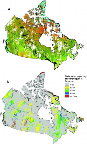
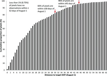
We generated a national 2010 annual BAP composite for Canada (Figure 3a) using the aforementioned rule-base and assessed the observation yield relative to our target DOY, August 1 (Figure 3b). Approximately 17% of pixels do not have BAP observations within ± 30 days of our target DOY; however, if the date range is expanded to ± 45 days, then only 4% of pixels have no BAP observations (Figure 4). There are some areas in the country (i.e., Rocky Mountains, central Saskatchewan, eastern Newfoundland), where pixels were obscured with persistent cloud in 2010 and yielded no cloud-free observations within a ± 62 day window of August 1; however, this accounts for less than 1% of pixels. To fill in these areas would require the development of either a proxy BAP composite or a multi-year BAP composite (Table 3). We generated a multi-year composite (Figure 5) wherein pixels with no observations within the ± 30 day window for 2010 were populated with BAP observations from 2009 and 2011.

FIG. 3. 2010 annual best available pixel (BAP) composite (A) using August 1 ± 30 days. Approximately 17% of pixels have no observations within that date range. The distance to target day of year (DOY; B) indicates the DOY distribution; less than 1% of pixels have no observations (no data).

FIG. 4. Observation yield for 2010 annual BAP composite for Canada.

FIG. 5. Multi-year BAP composite for Canada incorporating pixels from years 2009, 2010, 2011.

Annual BAP composites for Saskatchewan and Newfoundland: 1998–2012

BAP Observation Yield

For the annual image composites in Saskatchewan, 29% of pixels had observations from within ± 30 days of August 1 for all 15 years considered, whilst 74% of pixels have 13 or more years of observations within the target date range. All pixels in Saskatchewan had at least seven years of observations within the target date range (Figure 6a). Approximately 86% of pixels in Saskatchewan have no consecutive years of missing data (i.e., they are either missing only 1 or no years of data) (Figure 7a). Of the 14% of pixels with consecutive years of missing data, approximately 11% have two consecutive years of missing data, whilst 3% of pixels have 3 or more consecutive years of missing data. The geometric fidelity of Landsat imagery and the SLC-off failure are major contributors to this 14% of pixels that have several consecutive years of missing data, since this situation is more common after 2003 (the year of the SLC failure), as the SLC-off no-data gaps recur spatially.

FIG. 6. The observation yield of BAP pixels that provide the basis for composite development for Saskatchewan (A) and Newfoundland (B).

FIG. 7. The number and spatial distribution for consecutive years of missing data for Saskatchewan (A) and Newfoundland (B).

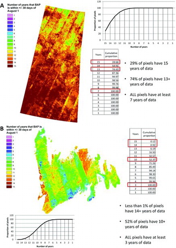
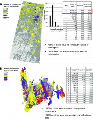
The observation yield from the annual composites for the island of Newfoundland contrasts with that in Saskatchewan: less than 1% of pixels had observations for 14 or more years within ± 30 days of August 1, whilst 52% of pixels have 10 or more years of observations within the target date range (Figure 6b). All pixels in Newfoundland had at least three years of observations within the target date range. Only about 18% of pixels in Newfoundland have no consecutive years of missing data, whilst 82% are missing two or more consecutive years of observations (Figure 7b). Similar to the results of our analysis in Saskatchewan, more pixels in Newfoundland had fewer consecutive years of missing data before 2003: 62% of pixels had no consecutive years of missing data before 2003, compared to only 24% of pixels after 2003.

Assessment of the Radiometric Consistency of Annual BAP Composites

Our assessment of the radiometric consistency of our annual BAP composites is summarized in Figure 8. The surface reflectance values in the annual BAP composite for both Saskatchewan and Newfoundland had strong correspondence with the single-date reference images in the near- and mid-infrared regions (bands 4, 5, 7), with R² > 0.79. Correspondence was lower in the visible wavelengths (bands 1, 2, and 3), with R² ranging from 0.60 to 0.75—likely as a result of atmospheric effects, which are more prevalent in these wavelengths. Moreover, despite the greater likelihood of clouds and cloud shadows in Newfoundland, which further limits the selection of the BAP and reduces the observation yield (Figures 6 and 7) compared to Saskatchewan, the Newfoundland composites had greater correspondence in the visible bands. Using a stable target (i.e., dense forest), the assessment of the annual BAP composites relative to an independent, single-date image indicates that no systematic artifacts are being introduced in the compositing process.

FIG. 8. Quality assessment of annual BAP composite for a sample path/row in Saskatchewan (p38r22) and Newfoundland (p3r26). For a randomly selected set of 500 pixels, surface reflectance values from a reference image are plotted against BAP composite surface reflectance values (reflectance values are scaled by 10000).

DISCUSSION

Pixel-Based Compositing Over Large Areas

A pixel-based image compositing approach has been proposed to address information needs associated with forest ecosystem science and monitoring in the Canadian context. Herein, we demonstrate the approach over large areas by presenting an annual BAP composite for Canada generated with Landsat data for the year 2010 and annual BAP time-series from 1998 to 2012 for the province of Saskatchewan and the island of Newfoundland. The compositing approach we present is inherently flexible, and the rules used for compositing can, in theory, be adjusted to accommodate a range of information needs (Table 4). The parametric scoring mechanisms for selecting BAP observations can be adjusted to give more or less weight to particular sensors, DOY, or the influence of clouds and haze according to specific information needs or application requirements, and this flexibility is one of the key advantages of the scoring mechanism used (Griffiths et al. 2013).

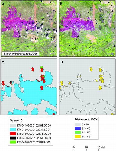
As indicated in our methods, we consider images acquired within ± 62 days of the target DOY with less than 70% cloud cover as viable candidates for compositing. However, given our knowledge of phenology and growing season length for much of the forested area of Canada, we limit our final composites to BAP observations that are within ± 30 days of our target DOY. We assign all BAPs from outside this temporal window as “no data”. We would then attempt to fill these “no data” pixels with proxy values derived using a time series approach or by generating a multi-year composite (Figure 5). The majority of BAP observations in the example presented in Figure 9 came from a Landsat-5 TM image acquired on day 210 (July 29), 2010 (LT50440202010210EDC00; Figure 9a). Pixels with clouds and cloud shadows in this image were identified with Fmask, and a distance to cloud score was assigned. In the final BAP composite (Figure 9b), these pixels were filled using observations from a number of different Landsat scenes (Figure 9c). Observations from images acquired outside the August 1 ± 30 day window (Figure 9d) are visibly different from the surrounding pixels, clearly demonstrating the need to constrain the DOY range.

Characteristics relevant to particular geographic regions, such as persistence of cloud cover, topography, dynamism of landscape processes, phenology, and Landsat data availability, are important considerations when applying a compositing approach. Likewise, different information needs (e.g., disturbance mapping, estimation of biophysical parameters) may dictate different compositing strategies, target dates, and compositing rules that are specific to the application (Table 4). Usually, there are trade-offs to be made in producing composite products. In general, it is desirable to generate composites that have consistent phenology with minimal “no data” pixels that best represent the phenomenon of interest (e.g., land cover classes, forest structural attributes, or specific disturbance events). These trade-offs may be location or application specific. For example, in northern Canada, a narrower DOY range for composite development is required to capture the shorter growing season in this area. Although a narrow date range in theory would reduce the probability of obtaining a cloud-free observation, the 80% overlap between Landsat scenes in the north (Wulder and Seemann 2001) ensures sufficient observations for annual BAP composites at this latitude. To enable the characterization of discrete disturbance events such as wildfires, it may be preferable to have a DOY range that is referenced to the end of the fire season (Table 4). Similarly, to characterize disturbances related to insects, the DOY range would very much depend on the type of damage requiring detection (i.e., a defoliator versus a bark beetle). An example of a program-specific information need is that of the National Deforestation Monitoring System (NDMS), which uses remotely sensed data to help create an estimate of anthropogenic change from a forest to a non-forest land use. NDMS is a sample-based program that produces national estimates of deforestation for a variety of clients; however, the mapping process could benefit from increased automation. The detection of possible deforestation events requires two core dates of imagery, typically bracketing a five year time period. The mapping process could be performed more efficiently by having access to two national annual BAP composites, which would allow for the display of various band combinations and the generation of a change enhanced image between the two composite years.

Fire is the primary natural disturbance agent in most boreal forests (Bond-Lamberty et al. 2007), and high inter-annual variability in the area burned, combined with large insect outbreaks, can have a profound influence on the greenhouse gas balance of Canada's forests (Kurz et al. 2008). Monitoring these types of natural disturbances requires acquisition of imagery before and after the disturbance to best detect spectral response changes that are in turn used to derive the spatial location, area, and magnitude of the disturbance. Fire is a random event that can occur over a broad temporal window from spring to late fall. Presently, a national annual map of areas burned in Canada is generated by compiling the best available information on burned areas from a variety of data sources such as Landsat TM or ETM+ imagery, SPOT VEGETATION, as well as data from provincial/territorial government fire management agencies (de Groot et al. 2007; Natural Resources Canada 2014). When the presence of cloud or smoke prevents the selection of a Landsat image, the burn polygon is extracted from fire agency data which may or may not be as accurate as what could be mapped from Landsat. Implementation of the BAP concept could potentially increase the likelihood of having a suitable cloud-free image for mapping burned areas.

The mapping of severe insect disturbances using remotely sensed data is an application that is highly time sensitive since the manifestation and detectability of damage varies by causal agent and time of year (Hall et al. 2006; Hicke et al. 2012). Particularly with insect defoliation, the opportunity to acquire cloud-free Landsat images may be confined to two or three satellite passes in the growing season (Hall et al. 2006). This very narrow temporal window can limit the use of optical satellite imagery for operational mapping of defoliation events. The potential to create cloud-free BAP composites from Landsat and Sentinel-2, with a three and five day revisit cycle could greatly increase the prospects of having suitable pre- and post-outbreak images for mapping of insect disturbances.

The most versatile compositing approach would have the entire Landsat image archive of Canada accessible on demand. Then, for any given information need, a customized rule-base could be constructed and implemented to create a suitable BAP composite. In this way, users bring their algorithms (and their information needs) to the data, rather than the opposite, where multiple users are downloading and replicating the Landsat archive of Canada in order to generate data products independently to support their information needs. Examples of this capacity include the NASA Earth Exchange (NEX) (Nemani et al. 2011), Google Earth Engine (Hansen et al. 2013), and Geoscience Australia (Geoscience Australia 2014). While such versatility is the ultimate goal, initial efforts are required to demonstrate pixel-based compositing over large areas, evaluate annual pixel-based composite products, and assess the potential for annual pixel-based composite products to support time-series applications.

TABLE 4 Examples of different information requirements and associated compositing criteria

Application area	Date range	Rule-base
Land cover	Aug 1 ± 30 days	Sensor
		Day of year
		Distance to cloud/cloud shadow
		Opacity
Forest structural attribution (height, volume, biomass)	Aug 1 ± 30 days	Sensor
		Day of year
		Distance to cloud/cloud shadow
		Opacity
Deforestation monitoring	Sep 1 +30, −60 days	Sensor
		Day of year
		Distance to cloud/cloud shadow
		Opacity
		Pixel temporal grouping
Wildfires	Nominally	Sensor
	Aug 20 to Oct 10	Day of year
	Pre- and post-burn image dates are influenced by early or late season burns	Distance to cloud/cloud shadow
		Opacity
		Date of end fire date
Insects	Variable depending on insect	Sensor
		Day of year
		Distance to cloud/cloud shadow
		Opacity
		Type of damage: eg., defoliator vs bark beetle based on agency aerial survey

Issues and Opportunities

Canada's large size and geographic complexity pose significant challenges for a pixel-based compositing approach. Primarily, the probability of cloud-free observations is a complex combination of regional weather conditions, acquisition scheduling, and historic downlink activity, among other issues (White and Wulder 2013). When it comes to scheduling, the conterminous United States (CONUS) has preferential data acquisition under the Landsat program (Kovalskyy and Roy 2013), with approximately 831,318 images for 459 unique path/rows for the period 1972–2012. For that same time period, Canada, as a strong International Cooperator in the Landsat program and with close proximity to CONUS, has approximately 605,000 images in the archive for 1224 unique path/rows (White and Wulder 2013). With this lower total number of images also comes a lower probability of cloud-free imagery. Given the large size of Canada and the need to monitor terrestrial ecosystems in a way that is systematic, consistent, transparent, and repeatable, BAP compositing offers the potential to increase the availability of cloud-free EO observations at a spatial resolution that can support monitoring requirements, however, the challenge of acquiring complete spatial and temporal coverage over large and geographically complex areas remains. With Landsat-8, a more globally inclusive data acquisition plan has been implemented that captures the majority of terrestrial WRS-2 path/rows within the satellite's orbit each day (Roy et al. 2014).

Through our product development, it is clear that the observation yield for our standard rule-base varies markedly in different regions of the country. Newfoundland is more prone to cloud cover, resulting in lower annual observation yield and the BAP compositing approach is most challenging in environments that are prone to cloud cover and haze. In such circumstances, leveraging the time series of Landsat is an important consideration. Saskatchewan may have fewer issues associated with cloud cover, but has a very dynamic natural disturbance regime, which is also challenging if the information need is to characterize discrete disturbance events.

The issue of “missing data” (i.e., pixels that have no BAP observations within the specified DOY range) requires specific attention. This is especially true for areas where cloud and haze conditions limit opportunities for pixels to meet the criteria for consideration as BAPs. These data gaps limit applications that require spatially exhaustive and location-specific coverage. Therefore, alternate methods are required to populate missing data. As presented in the lexicon for pixel-based image composites, the BAP approach could produce multi-year composite products or proxy-value composites depending on the information needs of the application. Multi-year composite methods, while simpler to develop, might be suitable for generating products for national reporting for specific time windows, while more complex methods for developing proxy-value products are needed for annual monitoring and modeling applications. In such cases, detection of change events in the pixel's spectral trajectory is a necessary precursor to the generation of proxy-value composites. For the development of proxy composites, the distribution of BAP observations within the 15-year period is also important: theoretically it is simpler to assign proxy values to single years of missing data interspersed in a time series of observations, than it is to assign proxy values to five consecutive years of missing data. Further development is needed in this area for operational implementation over large areas.

FIG. 9. Areas of cloud in a single-date image (LT50440202010210EDC00) (A) are replaced with cloud-free observations in the annual BAP composite for 2010 (B). The composite uses observations from several unique images (C), with the greatest difference visible for those images acquired outside the August 1 ± 30 day window (D).

Herein, we focused on forest ecosystem science and monitoring needs of the Canadian Forest Service. The goal was to create satellite-based image composite products that could expand the current sample-based NFI monitoring approach and provide spatially explicit information on forest dynamics for carbon accounting as well as a myriad of other information needs in Canada that would benefit from wall-to-wall image and data products with an annual time stamp. In the case of the NFI, satellite-based analyses are needed when plot density or temporal coverage is insufficient to meet the monitoring and reporting requirements at regional and national levels, such as can occur in northern Canada (Falkowski et al. 2009). For the products presented, we selected compositing parameters to support key forest ecosystem monitoring needs— characterization of land cover and land cover change, and attribution of forest structural parameters. Further research is needed to optimize the parameters for more specific applications. For example, an alternate DOY or narrower phenological window for identifying BAPs may result in improved land cover classification accuracy or improved predictions of structural parameters at the expense of areal coverage (i.e. more missing data). For time sensitive applications such as monitoring disturbances (e.g. fire, insect defoliation), imagery is required following the disturbance. Often, there is a very small window for detection and the optimal timing can vary by disturbance type. Capacity to generate products for such applications is currently limited by the frequency with which images are collected, but this limitation may be addressed with future sensors, with especial interest in the capacity of combined Sentinel-2 and Landsat 8 applications. Both Sentinel 2's remain to be launched and the complementarity of the measurements yet to be determined, as well as the nature of the data access. Opportunities for virtual constellations notwithstanding, continuity of Landsat measures remains of the highest priority, and the integration of Landsat-8 and Sentinel-2 observations into the BAP compositing process is an issue requiring further research.

Herein we have made some recommendations concerning how to best link compositing decisions to the desired use of the composite; however, further research may help to optimize these decisions across a broader range of applications. While our efforts to date have focused on information needs of the Canadian Forest Service (specifically, NFI and carbon accounting), monitoring, reporting, and science-based policy support are core activities of several other federal agencies in Canada. Each organization has sector-specific objectives associated with terrestrial monitoring, and while these objectives can often be met using the same or similar data, in some cases, optimization may improve product suitability for more specific information requirements (e.g. wetlands and agricultural monitoring).

CONCLUSIONS

The approach and products presented in this paper demonstrate that annual BAP compositing is possible for large areas and for time series application in the Canadian context. This is the first time that an annual BAP composite has been generated from Landsat imagery for all of Canada. In addition, annual BAP time-series extending from 1998 to 2012 were produced for Saskatchewan and the island of Newfoundland to support the further development of ecosystem monitoring applications. An important limitation for the application of annual BAP products to derive forest ecosystem information products (i.e., land cover, land cover change, and structural estimation) is missing data—pixels with no observations due to clouds, cloud shadows, sensor issues (SLC-off), or restricted acquisition period. In the future, it is expected that these limitations will be mitigated with increased coverage from future satellite sensors. However, to address historical and current information needs, further research is necessary to develop multi-year and BAP proxy-value composites targeted to specific monitoring applications. Future research will focus on developing approaches for using a time series of BAP proxy-value composites to generate information products for land cover, land cover change, and forest structure.

Additional information

Funding

This research was undertaken as part of the “National Terrestrial Ecosystem Monitoring System (NTEMS): Timely and detailed national cross-sector monitoring for Canada” project jointly funded by the Canadian Space Agency (CSA) Government Related Initiatives Program (GRIP) and the Canadian Forest Service (CFS) of Natural Resources Canada.

Notes

https://landsat.usgs.gov/CDR_ECV.php

http://landsat.usgs.gov/PLSRP_Tables.php

REFERENCES

- Bond-Lamberty, B., Peckham, S.D., Ahl, D.E., and Gower, S.T. 2007. Fire as a dominant driver of central Canadian boreal forest carbon balance. Nature Letters, Vol. 450: pp. 89–92.
- Broich, M., Hansen, M.C., Potapov, P., Adusei, B., Lindquist, E., and Stehman, S.V. 2011. Time series analysis of multi-resolution optical imagery for quantifying forest cover loss in Sumatra and Kalimantan, Indonesia. International Journal of Applied Earth Observation and Geoinformation, Vol. 13: pp. 277–291.
- Canadian Council of Forest Ministers. 1995. Defining sustainable forest management: A Canadian approach to criteria and indicators. Available online: http://cfs.nrcan.gc.ca/publications?id=10217
- Chander, G., Markham, B.L., and Helder, D.L. 2009. Summary of current radiometric calibration coefficients for Landsat MSS, TM, ETM+ and EO-1 ALI sensors. Remote Sensing of Environment, Vol. 113: pp. 893–903.
- Chavez, P.S. 1988. An improved dark-object subtraction technique for atmospheric scattering correction of multispectral data. Remote Sensing of Environment, Vol. 24(No. 3): pp. 459–479.
- Chen, G., Wulder, M.A., White, J.C., Hilker, T.H., and Coops, N.C. 2012. Lidar calibration and validation for geometric-optical modeling with Landsat. Remote Sensing of Environment, Vol. 124: pp. 384–393.
- Cihlar, J., Manak, D., and D’Iorio, M. 1994. Evaluation of compositing algorithms for AVHRR data over land. IEEE Transactions on Geoscience and Remote Sensing, Vol. 32(No. 2): pp. 427–436.
- de Groot, W.J., Landry, R., Kurz, W.A., Anderson, K.R., Englefield, P., Fraser, R., Hall, R.J., Raymond, D., Decker, V., Lynham, T.J., Banfield, E., and Pritchard, J.M. 2007. Estimating direct carbon emissions from Canadian wildland fires. International Journal of Wildland Fire, Vol. 16(No. 5): pp. 593–606.
- Department of Forest Resources and Agrifoods. 2003. Provincial sustainable forest management strategy. Government of Newfoundland and Labrador. Available online: http://www.nr.gov.nl.ca/nr/forestry/manage/sfm.pdf
- Drusch, M., Del Bello, U., Carlier, S., Colin, O., Fernandez, V., Gascon, F., Hoersch, B., Isola, C., Laberinti, P., Martimort, P., Meygret, A., Spoto, F., Sy, O., Marchese, F., and Bargellini, P. 2012. Sentinel-2: ESA's optical high-resolution mission for GMES operational services. Remote Sensing of Environment, Vol. 120: pp. 25–36.
- Du, Y., Cihlar, J., Beaubien, J., and Latifovic, R. 2001. Radiometric normalization, compositing, and quality control for satellite high resolution image mosaics over large areas. IEEE Transactions on Geoscience and Remote Sensing, Vol. 39: pp. 623–634.
- Falkowski, M.J., Wulder, M.A., White, J.C., and Gillis, M.D. 2009. Supporting large-area, sample-based forest inventories with very high spatial resolution satellite imagery. Progress in Physical Geography, Vol. 33(No. 3): pp. 403–423.
- Feng, M., Sexton, J.O., Huang, C., Masek, J.G., Vermote, E.F., Gao, F., Narasimhan, R., Channan, S., Wolfe, R.E., and Townshend, J.R. 2013. Global surface reflectance products from Landsat: Assessment using coincident MODIS observations. Remote Sensing of Environment, Vol. 134: pp. 276–293.
- Flood, N. 2013. Seasonal composite Landsat TM/ETM +images using the Medoid (a multi-dimensional median). Remote Sensing, Vol. 5(No. 12): pp. 6481–6500.
- Flood, N., Danaher, T., Gill, T., Gillingham, S. 2013. An operational scheme for deriving standardised surface reflectance from Landsat TM/ETM+ and SPOT HRG Imagery for Eastern Australia. Remote Sensing, Vol. 5: pp. 83–109.
- Gao, F., Masek, J., Schwaller, M., Hall, F. 2006. On the blending of the Landsat and MODIS surface reflectance: predicting daily Landsat surface reflectance. IEEE Transactions on Geoscience and Remote Sensing, Vol. 44: pp. 2207–2218.
- Geoscience Australia. 2014. The future of the Landsat archive. Available online: http://www.ga.gov.au/earth-observation/accessing-satellite-imagery/future-of-landsat-archive.html
- Gillis, M.D. 2001. Canada's National Forest Inventory (responding to current information needs). Environmental Monitoring and Assessment, Vol. 67: pp. 121–129.
- Gillis, M.D., Omule, A.Y., and Brierley, T. 2005. Monitoring Canada's forests: The National Forest Inventory. The Forestry Chronicle, Vol. 81: pp. 214–221.
- Griffiths, P., van der Linden, S., Kuemmerle, T., and Hostert, P. 2013. A pixel-based Landsat compositing algorithm for large area land cover mapping. Journal of Selected Topics in Applied Earth Observations and Remote Sensing, Vol. 6(No. 5): pp. 2088–2101.
- Guindon, B., and Edmonds, C.M. 2002. Large-area land cover mapping through scene-based classification compositing. Photogrammetric Engineering and Remote Sensing, Vol. 68: pp. 589–596.
- Gutman, G., Huang, C., Chander, G., Noojipady, P., and Masek, J.G. 2013. Assessment of the NASA-USGS Global Land Survey (GLS) datasets. Remote Sensing of Environment, Vol. 134: pp. 249–265.
- Haley, D. and Luckert, M.K. 1990. Forest tenures in Canada: A framework for policy analysis. Ottawa, Forestry Canada: Information Report E-X-43, 104 p.
- Hall, R.J., Skakun, R.S. Skakun, and Arsenault, E.J. 2006. Remotely sensed data for mapping insect defoliation. pp. 85–111 in M.A. Wulder and S.E. Franklin (editors). Forest Disturbance and Spatial Pattern: Remote Sensing and GIS Approaches. Taylor and Francis. CRC Press.
- Hansen, M.C., and Loveland, T.R. 2012. A review of large area monitoring of land cover change using Landsat data. Remote Sensing of Environment, Vol. 122: pp. 66–74.
- Hansen, M.C., Potapov, P.V., Moore, R., Hancher, M., Turubanova, S.A., Tyukavina, A., Thau, D., Stehman, S.V., Goetz, S.J., Loveland, T.R., Kommareddy, A., Egorov, A., Chini, L., Justice, C.O., and Townshend, J.R. G. 2013. High resolution global maps of 21st-century forest cover change. Science, Vol. 342: pp. 850–853.
- Hansen, M.C., Roy, D.P., Lindquist, E., Adusei, B., Justice, C.O., Alstatt, A. 2008. A method for integrating MODIS and Landsat data for systematic monitoring of forest cover and change in the Congo Basin. Remote Sensing of Environment, Vol. 112(No. 5): pp. 2495–2513.
- Helmer, E.H., Ruzycki, T.S., Wunderle, J.M., Vogesser, S., Ruefenacht, C., Kwit, C., Brandeis, T.J., and Ewert, D.N. 2010. Mapping tropical dry forest height, foliage height profiles and disturbance type and age with a time series of cloud-cleared Landsat and ALI image mosaics to characterize avian habitat. Remote Sensing of Environment, Vol. 114: pp. 2457–2473.
- Hicke, J.A., Allen, C.D., Desai, A.R., Dietze, M.C., Hall, R.J., Hogg, E.H., Kashian, D.M., Moore, D., Raffa, K., Sturrock, R., and Vogelmann, J. 2012. Effects of biotic disturbances on forest carbon cycling in the United States and Canada. Global Change Biology, Vol. 18(No. 1): pp. 7–34.
- Hofgaard, A., Tardif, J., and Bergeron, Y. 1999. Dendroclimatic response of Picea mariana and Pinus banksiana along a latitudinal gradient in the eastern Canadian boreal forest. Canadian Journal of Forest Research, Vol. 29: pp. 1333–1346.
- Holben, B. 1986. Characteristics of maximum-value composite images from temporal AVHRR data. International Journal of Remote Sensing, Vol. 7: pp. 1417–1434.
- Irons, J.R., Dwyer, J.L., and Barsi, J.A. 2012. The next Landsat satellite: the Landsat Data Continuity Mission. Remote Sensing of Environment, Vol. 122: pp. 11–21.
- Ju, J., Roy, D.P., Shuai, Y., and Schaaf, C. 2010. Development of an approach for generation of temporally complete daily nadir MODIS reflectance time series. Remote Sensing of Environment, Vol. 114(No. 1): pp. 1–20.
- Justice, C.O., Townshend, J.R. G., Vermote, E.F., Masuoka, E., Wolfe, R.E., Saleous, N., Roy, D.P., and Morisette, J.T. 2002. An overview of MODIS land data processing and product status. Remote Sensing of Environment, Vol. 83: pp. 3–15.
- Kaufman, Y.J., Tanre, D., Remer, L.A., Vermote, E.F., Chu, A., and Holben, B.N. 1997. Operational remote sensing of tropospheric aerosol over the land from EOS-MODIS. Journal of Geophysical Research-Atmosphere, Vol. 102: pp. 17051–17068.
- Kennedy, R., Yang, Z., and Cohen, W.B. 2010. Detecting trends in forest disturbance and recovery using yearly Landsat time series: 1. LandTrendr—temporal segmentation algorithms. Remote Sensing of Environment, Vol. 114: pp. 2897–2910.
- Kovalskyy, V., and Roy, D.P. 2013. The global availability of Landsat 5 TM and Landsat 7 ETM+ land surface observations and implications for global 30 m Landsat data product generation. Remote Sensing of Environment, Vol. 130: pp. 280–293.
- Kurz, W.A., Stinson, G., Rampley, G.J., Dymond, C.C., and Neilson, E.T. 2008. Risk of natural disturbances makes future contribution of Canada's forests to the global carbon cycle highly uncertain. Proceedings of the National Academy of Sciences of the United States of America, Vol. 105: pp. 1551–1555.
- Kurz, W.A., Dymond, C.C., White, T.M., Stinson, G., Shaw, C.H., Rampley, G.J., Smyth, C., Simpson, B.N., Neilson, E.T., Trofymow, J.A., Metsaranta, J., and Apps, M.J. 2009. CBM-CFS3: A model of carbon dynamics in forestry and land-use change implementing IPCC standards. Ecological Modelling, Vol. 220: pp. 480–504.
- Lindquist, E.J., Hansen, M.C., Roy, D.P., and Justice, C.O. 2008. The suitability of decadal image data sets for mapping tropical forest cover change in the Democratic Republic of Congo: implications for the global land survey. International Journal of Remote Sensing, Vol. 29: pp. 7269–7275.
- Masek, J.G., Vermote, E.F., Saleous, N., Wolfe, R., Hall, F.G., Huemmrich, F., Gao, F., Kutler, J., and Lim, T.K. 2006. A Landsat surface reflectance data set for North America, 1990–2000. IEEE Geoscience and Remote Sensing Letters, Vol. 3(No. 1): pp. 68–72.
- McKenney, D., Pedlar, J.H., Papadopol, P., and Hutchinson, M.F. 2006. The development of 1901-2000 historical monthly climate models for Canada and the United States. Agricultural and Forest Meterology, Vol. 138(Nos. 1–4): pp. 69–81.
- Natural Resources Canada. 2013. The State of Canada's Forests Annual Report 2013. Canadian Forest Service, Headquarters, Ottawa. 56 p. Available online: https://cfs.nrcan.gc.ca/publications?id=35191
- Natural Resources Canada. 2014. FireMARS [Internet]. Ottawa, ON: Nat. Resour. Can. Available online: http://www.nrcan.gc.ca/forests/ fire/13159
- Nemani, R., Votava, P., Michaelis, A., Melton, F., and Milesi, C. 2011. Collaborative supercomputing for global change science. EOS Transactions, Vol. 92(No. 13): pp. 109–110.
- Potapov, P., Turubanova, S., and Hansen, M.C. 2011. Regional-scale boreal forest cover and change mapping using Landsat data composites for European Russia. Remote Sensing of Environment, Vol. 115: pp. 548–561.
- Potapov, P., Turubanova, S., Hansen, M.C., Adusei, B., Broich, M., Alstatt, A., Mane, L., and Justice, C.O. 2012. Quantifying forest cover loss in Democratic Republic of the Congo, 2000-2010, with Landsat ETM+ data. Remote Sensing of Environment, Vol. 122: pp. 106–116.
- Roy, D.P. 2000. The impact of misregistration upon composited wide field of view satellite data and implications for change detetcion. IEEE Transactions on Geoscience and Remote Sensing, Vol. 38: pp. 2017–2032.
- Roy, D.P., Ju, J., Kline, K., Scaramuzza, P.L., Kovalskyy, V., Hansen, M., Loveland, T.R., Vermote, E., and Zhang, C. 2010. Web-enabled Landsat Data (WELD): Landsat ETM+ composited mosaics of the conterminous United States. Remote Sensing of Environment, Vol. 114: pp. 35–49.
- Roy, D.P., Wulder, M.A., Loveland, T.R., Woodcock, C.E., Allen, R.G., Anderson, M.C., Helder, D., Irons, J.R., Johnson, D.M., Kennedy, R., Scambos, T.A., Schaaf, C.B., Schott, J.R., Sheng, Y., Vermote, E.F., Belward, A.S., Bindschadler, R., Cohen, W.B., Gao, F., Hipple, J.D., Hostert, P., Huntington, J., Justice, C.O., Kilic, A., Kovalskyy, V., Lee, Z.P., Lymburner, L., Masek, J.G., McCorkel, J., Shuai, Y., Trezza, R., Vogelmann, J., Wynne, R.H., and Zhu, Z. 2014. Landsat-8: Science and product vision for terrestrial global change research. Remote Sensing of Environment. Vol. 145: pp. 154–172.
- Saskatchewan Ministry of Environment. 2012. 2012 Report on Saskatchewan Forests. Government of Saskatchewan. Available online: http://www.environment.gov.sk.ca/forests.
- Schmidt, G.L., Jenkerson, C.B., Masek, J., Vermote, E., and Gao, F. 2013. Landsat ecosystem disturbance adaptive processing system (LEDAPS) algorithm description. U.S. Geological Survey Open-File Report 2013–1057, 17 p. Available online: http://pubs.usgs.gov/of/2013/1057/
- Townshend, J.R. G., and Justice, C.O. 1988. Selecting the spatial resolution of satellite sensors required for global monitoring of land transformations. International Journal of Remote Sensing, Vol. 9(No. 2): pp. 187–236.
- Townshend, J.R., Masek, J.G., Huang, C., Vermote, E.F., Gao, F., Channan, S., Sexton, J.O., Feng, M., Narasimhan, R., Kim, D., Song, K., Song, D., Song, X., Noojipady, P., Tan, B., Hansen, M.C., Li, M., and Wolfe, R.E. 2012. Global characterization and monitoring of forest cover using Landsat data: opportunities and challenges. International Journal of Digital Earth. Vol 5(No. 5): pp. 373–397.
- Tucker, C.J., Grant, D.M., and Dykstra, J.D. 2004. NASA's global orthorectified Landsat data set. Photogrammetric Engineering and Remote Sensing, Vol. 70: pp. 313–322.
- United States Geological Survey. 2013. Product Guide Landsat Climate Data Record (CDR) Surface Reflectance. Version 3.4. December, 2013. Available online: http://landsat.usgs.gov/documents/cdr_sr_product_guide.pdf
- van Aardt, J.A. N., and Wynne, R.H. 2001. Spectral separability among six southern tree species. Photogrammetric Engineering and Remote Sensing, Vol. 67(No. 12): pp. 1367–1375.
- Vermote, E.F., Tanre, D., Deuze, J.L., Herman, M., and Morcrette, J.-J., 1997, Second simulation of the satellite signal in the solar spectrum, 6S—An overview. IEEE Transactions on Geoscience and Remote Sensing, Vol. 35(No. 3): pp. 675–686.
- White, J.C., and Wulder, M.A. 2013. The Landsat observation record of Canada: 1972-2012. Canadian Journal of Remote Sensing, Vol. 39: pp. 455–467.
- Wijedesa, L.S., Sloan, S., Michelakis, D.G., and Clements, G.R. 2012. Overcoming limitation with Landsat imagery for mapping of peat swamp forests in Sundaland. Remote Sensing, Vol. 4(No. 9): pp. 2595–2618.
- Wolfe, R.E., Roy, D.P., and Vermote, E. 1998. MODIS land data storage, gridding, and compositing methodology: Level 2 grid. IEEE Transactions on Geoscience and Remote Sensing, Vol. 36: pp. 1324–1338.
- Woodcock, C.E., Allen, R., Anderson, M., Belward, A., Bindschadler, R., Cohen, W., Gao, F., Goward, S.N., Helder, D., Helmer, E., Nemani, R., Oreopoulos, L., Schott, J., Thenkabail, P.S., Vermote, E.F., Vogelmann, J., Wulder, M.A., and Wynne, R. 2008. Free access to Landsat imagery. Science, Vol. 320(No. 5874): p. 1011.
- Wulder, M.A., and Seemann, D. 2001. Spatially partitioning Canada with the Landsat Worldwide Referencing System. Canadian Journal of Remote Sensing, Vol. 27(No. 3): pp. 225–231.
- Wulder, M.A., Kurz, W., and Gillis, M.D. 2004. National level forest monitoring and modelling in Canada. Progress in Planning, Vol. 61: pp. 365–381.
- Wulder, M.A., Campbell, C., White, J.C., Flannigan, M., and Campbell, I.D. 2007a. National circumstances in the international circumboreal community. The Forestry Chronicle, Vol. 83(No. 4): pp. 539–556.
- Wulder, M.A., White, J.C., Magnussen, S., and McDonald, S. 2007b. Validation of a large-area land cover product using purpose acquired airborne video. Remote Sensing of Environment, Vol. 106: pp. 480–491.
- Wulder, M.A., White, J.C., Cranny, M., Hall, R.J., Luther, J.E., Beaudoin, A., Goodenough, D.G., and Dechka, J.A. 2008. Monitoring Canada's forests. Part 1: Completion of the EOSD land cover project. Canadian Journal of Remote Sensing Vol. 34(No. 6m): pp. 549–562.
- Wulder, M.A., Masek, J.G., Cohen, W.B., Loveland, T.R., and Woodcock, C.E. 2012. Opening the archive: How free data has enabled the science and monitoring promise of Landsat. Remote Sensing of Environment, Vol. 122: pp. 2–10.
- Zhu, Z., and Woodcock, C.E. 2012. Object-based cloud and cloud shadow detection in Landsat imagery. Remote Sensing of Environment, Vol. 118: pp. 83–94.