A High Spatial Resolution Satellite Remote Sensing Time Series Analysis of Cape Bounty, Melville Island, Nunavut (2004–2018)

Abstract

Changes in vegetation have been observed in areas of the Arctic due to changing climate. This study examines a normalized difference vegetation index (NDVI) time series (2004–2018) of high spatial resolution satellite data (i.e., IKONOS, WorldView-2, WorldView-3) to determine if vegetation abundance has changed over the Cape Bounty Arctic Watershed Observatory, Melville Island, Nunavut. Image data were corrected to top-of-atmosphere reflectance and normalized for time series analysis using the pseudo-invariant feature (PIF) method. Percent vegetation cover measurements and indices derived from local climate data (growing degree days base 5 °C; GDD₅) were used to contextualize NDVI trends in different vegetation types and within active layer detachments (ALDs). NDVI showed similar patterns within the different vegetation types and across the ALDs. There was no significant change in NDVI nor in GDD₅ over time. However, there were statistically significant (p < 0.05) relationships between the GDD₅ and NDVI for all vegetation types. Using field measurements with high spatial resolution remote sensing data helps link changes in NDVI with changes to vegetation and earth surface processes. The challenges of integrating high spatial resolution satellite data from different sensors in a time series analysis are also discussed.

Résumé

Des modifications de la couverture végétale ont été observées dans des zones de l'Arctique en raison des changements climatiques. Cette étude consiste en l’analyze d’une série temporelle d’indice de végétation par différence normalisée (NDVI) (2004–2018) provenant de données satellitaires à haute résolution spatiale (IKONOS, WorldView-2, WorldView-3). L’étude vise à déterminer si des changements d’abondance de la végétation sont survenus dans la région de Cape Bounty Arctic Watershed Observatory (CBAWO), île Melville, Nunavut. Une correction atmosphérique de la réflectance TOA (top-of-atmosphère) et une normalization à l’aide de la méthode des attributs pseudo-invariants (« pseudo-invariant features » ou PIF) ont été appliquées aux données satellitaires afin de réaliser l’analyze de la série temporelle. Les pourcentages de couverture végétale et les indices dérivés des données climatiques locales (degrés-jours de croissance ou GDD₅) ont été utilisés pour contextualiser les tendances du NDVI observées dans différents types de végétation et au sein de zones affectées par des décrochements de couche active (ALD). Des patrons similaires du NDVI ont été observés dans les différents types de végétation et dans les ALDs. Aucun changement significatif du NDVI et du GDD₅ n’a été identifié pendant la période à l’étude. Cependant, des relations statistiquement significatives (p < 0.05) entre le GDD₅ et le NDVI ont été identifiées et ce, pour tous les types de végétation. L'utilisation de données de terrain, combinée à l’utilisation de données de télédétection à haute résolution spatiale, permet de relier les changements du NDVI aux changements de la végétation et à des processus de surface spécifiques. Les défis d’intégrer des données satellitaires à haute résolution spatiale provenant de différents capteurs dans une même analyze de séries temporelles sont également abordés.

Introduction

Warming in the Arctic is two to three times greater than the global average (Screen and Simmonds 2010; AMAP 2019; IPCC 2018). As a result, there is strong evidence of environmental change occurring in the High Arctic attributed to warming (Bjorkman et al. 2020; Davis et al. 2020; IPCC 2018; Overland et al. 2014); i.e., observations from coarse and intermediate spatial resolution satellite data have observed increases and decreases in vegetation indices, with increases (‘greening’) more prevalent than decreases (‘browning’) in Arctic vegetation over four decades (e.g., Bhatt et al. 2013; Bonney et al. 2018; Epstein et al. 2012; 2018; Ju and Masek 2016; Myers-Smith et al. 2020; Vickers et al. 2016). Additionally, field experiments that have simulated warming conditions (i.e., within sheltered enclosures) and/or increased snow cover (i.e., with snow fences) have shown that changes to climate can affect vegetation phenology, reproductive tendencies and height (e.g., Barrett et al. 2015; Barrett and Hollister 2016; Myers-Smith et al. 2011), vegetation cover (e.g., Elmendorf et al. 2012; Zamin et al. 2014) and species composition (Leffler et al. 2016). Likewise, long-term observational studies in areas of warming have shown that species composition has shifted (Edwards and Henry 2016; Kapfer et al. 2012) with an increase in shrub cover in some areas (e.g., Elmendorf et al. 2012; Fraser et al. 2014; Hill and Henry 2011; Hudson and Henry 2009; Myers-Smith et al. 2011).

Changes to vegetation and abiotic components (i.e., snow, water, ice and permafrost condition) of the vast and remote Arctic landscape can occur over very short distances (i.e., metres) calling for a combination of in-situ observations and high spatial resolution remote sensing data to detect and quantify environmental change over time. Spectral vegetation indices like the normalized difference vegetation index (NDVI) (Tucker 1979) have been used to track changes in vegetation ‘greenness’ across the Arctic. For example, products from the Advanced Very High Resolution Radiometer (AVHRR, l.1 km spatial resolution) and the Global Inventory Modeling and Mapping Studies (GIMMS, 8 km resolution) have used NDVI to track changes in vegetation at a circumpolar or continental scale (e.g., Bhatt et al. 2013, 2017; Epstein et al. 2012, 2018; Reichle et al. 2018; Vickers et al. 2016; Walker et al. 2012; Zhao et al. 2015). Studies at this resolution have shown that there has been a general greening trend through most of the Arctic since the 1980s, but there is evidence that the strength of this trend has been weakening in recent years (e.g., Bhatt et al. 2013, 2017; Vickers et al. 2016; Epstein et al. 2018).

Coarse spatial resolution satellite products are valuable for tracking Arctic vegetation change due to their long record and relatively high temporal frequency. However, recent comparisons with remote sensing data collected at intermediate spatial resolution (e.g., Landsat 30 m resolution) have suggested that there may be discrepancies between trends observed with different sensor products. Specifically, Ju and Masek (2016) found that the magnitude, heterogeneity and extent of greening differed between Landsat and AVHRR time series, while Raynolds et al. (2013) reported that greening trends observed with Landsat on Alaska’s North Slope were more spatially heterogeneous than those observed with AVHRR. Furthermore, this heterogeneity was driven by environmental factors that varied over small spatial scales (e.g., topography, glacial history, elevation, permafrost conditions, and soil conditions). Pattison et al. (2015) suggest that in some Arctic landscapes, satellite products with coarser spatial resolutions may fail to accurately capture trends on the landscape due to the influence of sub-pixel sized features/surfaces and the potential interference of shadows and standing water on the derivation of NDVI. This suggests that changes on the landscape may be better captured by imagery with a finer spatial resolution (i.e., resulting in decreased spectral mixing of surface types in an inherently heterogeneous environment).

In addition to tracking changes in undisturbed landscapes, coarser spatial resolution imagery may not be suited to tracking changes in disturbed landscapes, specifically when disturbances are sub-pixel in scale such as many permafrost disturbances. For example, active layer detachments (ALDs) occur when the active layer becomes unstable and slides downslope. This creates a scar zone with no vegetation at the top of the slope and a zone with compressed soil and vegetation at the base (Lewkowicz 2007). Though localized, the vegetation in the ALDs can be heavily disturbed and may take decades to return to pre-disturbance conditions (Cannone et al. 2010). In addition to the role vegetation plays in the Arctic carbon cycle through carbon sequestration, the removal of vegetation from the surface can change the amount of energy received by the soil below through changes in snow accumulation, albedo (Juszak et al. 2014) and shading (Juszak et al. 2016). Even large ALDs and retrogressive thaw slumps (RTS) are generally smaller than the cell size of satellite products like AVHHR or MODIS. Hence, high spatial resolution satellite data provide opportunities for locating and tracking changes in the landscape due to these disturbances.

The application of high spatial resolution imagery for time-series analysis in the Arctic is not as common as those with moderate or coarse resolutions as high spatial resolution data have only more recently become available. Further, unlike most of the coarser resolution products, high spatial resolution imagery must be contracted through a private sector data provider. In addition to the issue of cost, it can be difficult to acquire imagery during the short Arctic growing season due to often extensive and persistent cloud cover (Karlsen et al. 2018). Here, we analyze high spatial resolution multispectral data (IKONOS (4 m) and WorldView-2 (2 m), WorldView-3 (1.6 m)) collected from 2003–2018 at the Cape Bounty Arctic Watershed Observatory (CBAWO), Melville Island, Nunavut, Canada. Using these high spatial resolution multispectral data, local climate data and vegetation surveys in 2004 and 2017, we examine the trends observed in the high spatial resolution multispectral data in the context of changes in vegetation and climate at this High Arctic site.

In order to conduct this analysis, these remote sensing data must be normalized to account for different sensors, dates of acquisition and atmospheric conditions. These procedures must also be suited for application to high spatial resolution optical imagery, require no empirical atmospheric information (as these data are largely unavailable for remote areas), and be applicable in a High Arctic setting. As highlighted by Guay et al. (2014), there are challenges with using multiple sensors to track change, including differences in spatial and spectral resolutions and contrasting calibrations of spectral data which are sensor specific. Though time series with multiple Landsat sensors are common (e.g., Bonney et al. 2018; Edwards and Treitz 2017; Fraser et al. 2014; Ju and Masek 2016; Raynolds et al. 2013; Vickers et al. 2016), and there have been multi-sensor studies with different sensors (e.g., Simms and Ward 2013), time series combining IKONOS, WorldView-2 and WorldView-3 data are lacking.

Therefore, the objectives of this study are three-fold. First, we present an application and discussion of the use of the pseudo-invariant feature (PIF) method (Chen et al. 2005; Eckhardt et al. 1990; Heo and FitzHugh 2000; Hong and Zhang 2008; Schott et al. 1988) in a High Arctic setting to normalize data from different high spatial resolution sensors. Second, we analyze the time series to determine changes in greenness in the context of field data collected in a High Arctic environment at a landscape scale and in areas of disturbance. Finally, we compare the high spatial resolution time series analysis with an “upscaled” (i.e., spatially averaged) version of the high resolution (i.e., 2 m) time series to explore the advantages of high spatial resolution time series data for detecting change at landscape and local scales.

Data and Methods

Site Description

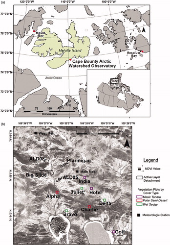
This research was conducted at the CBAWO, an interdisciplinary field research station located on Melville Island, Nunavut (74º55′ N, 109º35′ W; Figure 1a). Meteorological data have been collected at the CBAWO since 2003 at WestMet (Figure 1b). The typical growing season starts in early July, peaks in mid-late July with the onset of senescence early in August. The mean July temperature and precipitation between 2003 and 2018 was 5.4 °C and 22 mm respectively. The study site has three general vegetation types arranged along a soil moisture gradient, i.e., wet sedge, mesic heath tundra and polar semi-desert. These correspond in general to W1 (sedge/grass, moss wetland), G1 (rush/grass, forb, cryptogam tundra) and P1 (prostrate dwarf-shrub, herb tundra) respectively from the Circumpolar Arctic Vegetation Map (CAVM) (Walker et al. 2005). Though precipitation does deliver moisture to the landscape, snowmelt from semi-permanent snowbanks (associated with a shallow active layer) is an important source of water during the growing season for wet sedge areas. The polar semi-desert areas tend to be present on exposed uplands where vegetation tends to occur in moist depressions. The mesic areas tend to exhibit intermediate moisture.

Figure 1. (a) Map of Canada (inset) and the Cape Bounty Arctic Watershed Observatory in the Canadian High Arctic (basemap created using data from Statistics Canada (2011)); and b) WorldView-2 2012 NDVI image of the study area with plot identifiers (Alpha, Bravo, Charlie, Delta, Golf, Hotel, India, Juliet), active layer detachments (ALDs)(ALD05, ALD08, Big Slide, Ptarmigan) and meteorological stations (Main Met, West Met).

Satellite Multispectral Data

Image data were acquired during peak growing season (July 10 to August 2) and were relatively free of cloud and haze. The high spatial resolution satellite data used for these analyses are summarized in Table 1. Due to the pointable nature of the sensors (i.e., non-nadir look angles) changes in the bidirectional reflectance function may have had an impact on the measured reflectance. However, due to lack of anisotropic reflectance models for the vegetated surfaces at this latitude and the solar elevation angles being comparable (Table 1), surfaces were assumed to behave in a Lambertian fashion and maintain their reflectance regardless of look angle.

Table 1. High spatial resolution satellite metadata (IKONOS; WorldView-2 (WV2); WorldView-3 (WV3)) for images covering the Cape Bounty Arctic Watershed Observatory, Melville Island, Nunavut.

Date of Acquisition (DD/MM/YYYY)	Local Time	Pixel Size (m)	Bits per Pixel	Satellite	Solar Elevation Angle	Sensor Azimuth Angle	Sensor Elevation Angle
22/07/2004	14:31	4	11	IKONOS	35.2	91.5	70.7
02/08/2008	14:49	4	11	IKONOS	32.6	50.5	77.0
11/07/2010	14:39	4	11	IKONOS	37.2	88.5	79.4
15/07/2012	16:01	2	16	WV2	35.0	248.7	51.3
10/07/2014	18:01	2	16	WV2	36.2	243.7	62.5
28/07/2016	15:12	2	16	WV2	33.6	228.8	62.8
02/08/2018	16:44	1.6	16	WV3	31.8	307.7	71.2

Geometric Corrections

Geometric corrections were applied using ENVI 5.4.1 (hereafter ENVI) using seed tie points, rational polynomial coefficients, and a high resolution (1 m) digital elevation model (DEM). All images were resampled to 2 m spatial resolution to match the base image (WorldView-2 2016). The RMSE of the registrations were ∼2.1 IKONOS pixels (∼9 m). For additional details regarding the geometric correction, the reader is referred to Freemantle (2019).

Atmospheric Correction

Atmospheric correction removes the effects of selective scattering and absorption of different spectral wavelengths; a process that is necessary when biophysical variables are being extracted (Haboudane et al. 2002). Derivation of top-of-atmosphere (TOA) reflectance requires no information about the state of the atmosphere at image capture and thus has been used in multi-temporal and multi-sensor analyses (Laurent et al. 2011). In remote areas where atmospheric data are often unattainable (as in this study), TOA reflectance offers a suitable alternative for change detection studies. The approach described here normalizes for solar irradiance and is useful for reducing image-to-image differences (Taylor 2005) and has been described as a suitable approach given its simplicity and effectiveness across different sensor platforms (Dorigo et al. 2007). In this analysis, image data (i.e., brightness values (BVs)) for each sensor were corrected to TOA reflectance using equations 1(1) $$L_{\lambda \text{Pixel},\text{Band}}=\text{GAIN}\ast BV\ast \left(\frac{\text{abscal factor}}{\text{effective bandwidth}}\right)+\text{OFFSET}$$(1) and 2(2) $${\rho }_{\lambda \text{Pixel},\text{Band}}=\frac{L_{\lambda \text{Pixel},\text{Band}}\ast d_{ES}^2\ast \pi }{\mathit{Esu}{n}_{\lambda \text{Band}}\ast \hspace{0.17em}\text{cos}\hspace{0.17em}({\theta }_s)}$$(2) (Kuester 2016): (1) $$L_{\lambda \text{Pixel},\text{Band}}=\text{GAIN}\ast BV\ast \left(\frac{\text{abscal factor}}{\text{effective bandwidth}}\right)+\text{OFFSET}$$(1) where L_λPixel,Band is the absolute radiance at the sensor (W m⁻² sr⁻¹µm⁻¹); abscalfactor is a calibration factor specific to each band, sensor and year of acquisition (W m⁻²sr⁻¹); and effectivebandwidth is a band and sensor specific value for each bandwidth (µm). These values are provided with the metadata for each image. The GAIN and OFFSET values are band and sensor specific absolute radiometric calibration factors and are updated annually by the image providers (Kuester 2017). The radiance values are (L_λPixel,Band ) then converted to TOA reflectance (ρ_λPixel,Band) for each band using the following formula (Fleming 2001; Kuester 2016; NASA n.d.): (2) $${\rho }_{\lambda \text{Pixel},\text{Band}}=\frac{L_{\lambda \text{Pixel},\text{Band}}\ast d_{ES}^2\ast \pi }{\mathit{Esu}{n}_{\lambda \text{Band}}\ast \hspace{0.17em}\text{cos}\hspace{0.17em}({\theta }_s)}$$(2) where L_λPixel,Band is the absolute radiance (W m⁻² sr⁻¹µm⁻¹), d²_ES is the Earth-Sun distance (Astronomical Units), θ_s is the solar zenith angle (provided in the metadata of the imagery in degrees and subsequently converted to radians); Esun_λBand is the band averaged solar exoatmospheric irradiance (W m⁻² µm⁻¹) using the curve developed by Thuillier et al. (2003) (suggested sources for the curves are provided by the image provider, i.e., Kuester 2016; Taylor 2005; Thuillier et al. 2003; Updike and Comp 2010). All calculations were applied to the imagery using the Band Math Function in ENVI.

Image Normalization

After correcting all images to TOA reflectance, images were normalized using the PIF method (Chen et al. 2005; Garcia-Torres et al. 2014; Edwards and Treitz 2017; Heo and FitzHugh 2000; Hong and Zhang 2008; Schott et al. 1988). The PIF method was used successfully to normalize a Landsat NDVI time series at the CBAWO (Edwards and Treitz 2017), illustrating that it can be applied to intermediate spatial resolution data in a High Arctic setting. A linear regression relationship between PIF reflectance in the base image and the image to be normalized was applied to remove systematic differences between sensors and atmospheric conditions. Again, due to spatial resolution (i.e., 2 m), image quality (i.e., 0% cloud) and availability of dark pixels (i.e., exposed ice-free water), the 2016 WorldView-2 image was selected as the base image for normalization.

In order to minimize error due to factors like atmospheric thickness and shade (i.e., as a result of variable solar azimuth and elevation), PIF selection focused on areas that were relatively flat and of similar elevation to the areas of interest in the scene (Eckhardt et al. 1990). PIFs were drawn using the ‘ROI’ tool in ENVI. Bright PIFS (i.e., areas of exposed bedrock, sand, or very sparsely vegetated polar desert) were selected using knowledge of the landscape from previous field campaigns that included photos, field notes, and corresponding locations recorded using a global positioning system (GPS). Additional PIFs were selected using pixels classified as “bare/rock” in a land-cover classification from 2008 IKONOS data (Edwards and Treitz 2017; Gregory 2011).

The average PIF size was 28 pixels. Using multiple pixels in each PIF reduces the signal-to-noise ratios (Heo and FitzHugh 2000; Hope et al. 2007). Once all the PIFs had been selected, statistics were extracted in ENVI using the ‘Statistics for All ROIs’ tool. The mean reflectance of each PIF was then used for creating the regression equations (Table 2). In these equations, the additive component (i.e., intercept) accounts for the differences in atmospheric path radiance and the multiplicative component (i.e., slope) accounts for sun angle (zenith and azimuth), atmospheric attenuation and phase angle (Jensen 2016). The red and infrared bands were ‘stacked’ in a single multi-temporal dataset for analysis (i.e., to derive NDVI for each year).

Table 2. Normalization regressions for red (bands 3 and 5 for IKONOS and WorldView-2/3 respectively) and near infrared (NIR) spectral channels (bands 4 and 7 for IKONOS and WorldView-2/3 respectively).

Year	Red band (3/5)	r^2	NIR band (4/7)	r^2
2004	y = 1.01*b3 + 0.0102	0.95	y = 1.06*b4 + 0.0206	0.97
2008	y = 1.79*b3 + 0.0072	0.80	y = 1.82*b4 + 0.0517	0.83
2010	y = 1.01*b3 + 0.0172	0.96	y = 1.07*b4 + 0.0256	0.97
2012	y = 1.61*b5 − 0.0862	0.96	y = 1.53*b7 − 0.0618	0.96
2014	y = 1.13*b5 − 0.0507	0.92	y = 1.05*b7 − 0.0284	0.94
2018	y = 1.57*b5 + 0.0032	0.92	y = 1.57*b7 + 0.0059	0.96

Areas of high reflectance (i.e., bedrock outcrops, dry exposed soil) were used for the bright PIF targets (25 PIFS per image date) and areas of deep and ice free water (3–5 per image depending on ice coverage) were used for dark PIF targets. Due to a lack of suitable dark pixels in the 2004 image, dark PIFs were simulated by modifying 2010 PIF values. To do this, the average difference in TOA reflectance between the 24 bright PIFs that were common to 2010 and 2004 was added to the 2010 dark PIF values to simulate 2004 dark PIFs. This simulation was necessary to satisfy the assumption that PIF targets represent a range of BVs (Eckhardt et al. 1990). The image for 2010 was selected for modification because: (i) it had good quality dark PIFs; (ii) the 2004 and 2010 image data were collected with the same sensor; and (iii) the 2004 and 2010 image data were collected at the same time of day, hence they both had similar solar elevation and azimuth angles. The dark PIFs from 2010 were also selected because the regression equations for 2004 and 2010 with bright PIFs only were very similar, suggesting that the factors being normalized (i.e., atmospheric conditions, sensor calibrations, time of day, etc.) were similar.

Calculation and Extraction of NDVI Values for 2 m and ‘Upscaled’ Analysis

After normalization, NDVI values were calculated for each image (Tucker 1979). NDVI is widely used to quantify vegetation biophysical variables (e.g., biomass, percent vegetation cover (PVC), leaf area index) in Arctic environments (Bhatt et al. 2013; Vickers et al. 2016; Walker et al. 2012): (3) $$\mathrm{NDVI}=\frac{\mathrm{NIR}-\mathrm{RED}}{\mathrm{NIR}+\mathrm{RED}}$$(3) where RED and near infrared (NIR) represent reflectance in the red and near infrared wavelengths, respectively.

To track changes in vegetation greenness, GPS data collected in the field were used to locate and extract pixels from the image data that corresponded to the vegetation plots (boundaries collected in 2017) and ALDs (boundaries collected in 2010, see Rudy et al. 2013). For the four largest ALDs in the study area (Table 3), a buffer was applied 12 m inside the edge of the GPS delineated boundaries, in order to limit the inclusion of mixed pixels arising from any potential co-registration errors. Then, this buffer was used with the ALD boundaries to extract pixels within the scar zone (bare soil exposed) and the toe zone (where patches of vegetation and soil accumulated at the base of the ALDs) from each image to track change of each ALD separately (i.e., post 2007 when the ALDs occurred). The largest ALDs were selected because these would provide suitable comparisons to ‘upscaled’ data (i.e., to 30 m spatial resolution). However, it should be noted that these ALDs were much larger than the majority of ALDs in the study area. The ALDs were located on slope which were in the mesic tundra vegetation class at the top of the slope and transitioned into wet mesic tundra or wet sedge at the base of the slope.

Table 3. Characteristics of selected active layer detachments at the Cape Bounty Arctic Watershed Observatory, Melville Island, Nunavut.

ALD	Length (m)	Width (m)	Area (m2)	Morphology
Big Slide	684	177	60924	Elongate
ALD08	238	112	20115	Compact
Ptarmigan	361	75	19588	Elongate
ALD05	355	58	19281	Elongate

To investigate the change in NDVI across different vegetation types, NDVI values were extracted from field plots as well as from stratified random point samples from the three major vegetation types (i.e., pixel counts were proportional to vegetation type area). These pixel values (i.e., samples) were used to extract NDVI values for: (i) each vegetation type over the time series; and (ii) rock/bare ground (to serve as a test of the normalization procedures). The extent of the vegetation types for the stratified random sampling was based on a classification of the landscape into wet sedge, mesic heath tundra, polar semi-desert and rock using multi-temporal IKONOS data (July 4 and August 2, 2008) (Edwards and Treitz 2017; Gregory 2011). To investigate the effect that high spatial resolution data may have on quantifying vegetation change, the NDVI data were ‘upscaled’ to 30 m spatial resolution using the ‘Resize Data’ tool in ENVI (to simulate Landsat data). The values for these pixels were then extracted as described above. In cases where the random point samples generated to estimate changes over the landscape were within the same pixel extent, they were treated as one observation. Additionally, some points that were on the edge of the masked areas became masked areas when the data were ‘upscaled’, thereby resulting in a lower sample size than for the 2 m spatial resolution analysis.

Weather Data

Hourly above-ground air temperature and precipitation data have been collected annually at the WestMet weather station (i.e., 2003–2018) at the CBAWO (Beel et al. 2018). These measurements were used to calculate the growing degree days (GDDs) and the growing season length (GSL) as defined by the GDDs. GDD describes the surface thermal conditions above a threshold temperature related to vegetation growth (here, 5 °C after Carter 1998 and Weijers et al. 2013 for Arctic species). GDD is calculated as: (4) $${\mathrm{GDD}}_{\mathrm{base}}\mathrm{ }=\mathrm{ }\left(\frac{T_{\max }+T_{\min }}{2}\right)\mathrm{ }-\mathrm{ }{T}_{\mathrm{base}}\mathrm{ }=\text{ Average Daily Temperature }-\mathrm{ }{T}_{\mathrm{base}}$$(4) where GDD_base is the GDD at base temperature. Here, a base temperature of 5 °C was used (hereafter GDD₅). However, similar analyses were conducted for base temperatures of 0 and 3 °C and presented in the Supplemental Information. T_max and T_min are the daily maximum and minimum temperatures and T_base is the base temperature. It follows that GSL is the cumulative number of days with a positive GDD (i.e., where the average daily temperature exceeded the base temperature) between June and August (as in Weijers et al. 2013). These days need not be contiguous. Finally, precipitation data were used to determine the amount of rainfall preceding image acquisition. In addition to having the potential to influence vegetation growth, increased soil moisture or standing water can dampen surface reflectance (Jensen 2016) and influence vegetation spectral indices (Raynolds and Walker 2016).

Field Measurements: Percent Vegetation Cover

Plots established by Atkinson in 2003 and 2004 (Atkinson and Treitz 2012; 2013) were revisited in the summer of 2017. These plots were 1 ha in size (100 m x 100 m) and were distributed among the different vegetation types (Figure 1b). To estimate vegetation cover in these plots, the modified Braun-Blanquet method (Braun-Blanquet 1932; 1946; 1965; Table 4) was applied in 2004 and repeated in 2017. In comparison to the ITEX pin-drop quadrat method that captures great detail over a small area, the Braun-Blanquet method allows for quick estimation of dominant cover types, thereby capturing PVC variation over a large area. Described as an abundance-dominance scale and perhaps the most common ordinal scale used in plant ecology (McNellie et al. 2019), the Braun-Blanquet method has been applied successfully in the Arctic (e.g., Laidler et al. 2009; Walker et al. 2012; Atkinson and Treitz 2012; 2013) and has been shown to be comparable to pin-drop data in statistical analysis (e.g., Ricotta and Feoli 2013; Damgaard 2014) and other numerical analysis techniques (Hakes 1994). Plots with heterogeneous vegetation cover (i.e., increased variability) required more samples (Table 5). At each randomly selected location, a 0.5 m x 0.5 m quadrat (0.25 m²) was used to estimate PVC of vegetation functional groups (and species where possible) using the Braun-Blanquet scale (Table 4).

Table 4. Braun-Blanquet abundance-dominance (cover) scale (Braun-Blanquet, 1932).

Braun-Blanquet Cover Scale	Percent Vegetation Cover Range	Transformed Value (Tüxen and Ellenberg, 1937)
5	75-100 %	87.5
4	50-75 %	62.5
3	25-50 %	37.5
2	2-25 %	15.0
1	1-5 %	2.5
+	<1 %	0.1
R	≪ 1%	–
0	0	–

Table 5. Number of Braun-Blanquet observations per 1-hectare plot (and by plot quadrant) for 2004 and 2017.

Cover type	Plot	Number of Samples per Plot (Quadrant) 2004	Number of Samples per Plot (Quadrant) 2017
Polar semi-desert	Alpha (A)	80 (20)	40 (10)
	Charlie (C)	80 (20)	40 (10)
Mesic tundra	Golf (G)	72 (18)	40 (10)
	Hotel (H)	32 (8)	32 (8)
	India (I)	28 (7)	32 (8)
Wet sedge	Bravo (B)	24 (6)	24 (6)
	Delta (D)	20 (5)	24 (6)
	Juliet (J)	24 (6)	24 (6)

Results

Climate Analysis

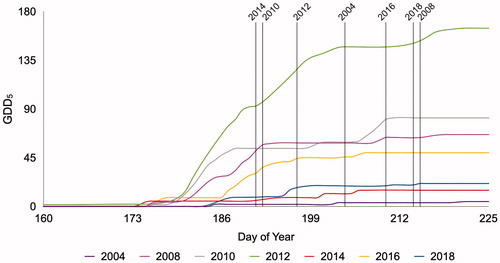
Figure 2 illustrates how GDD₅ corresponds to the dates of image acquisition and in context to the entire growing season. GDD₅ and GSL could vary considerably year by year, with 2012 having more than double the number of GDD₅ (126.6) than the next largest year (i.e., 2008 with 63.7 GDD₅). In addition, despite having one of the earlier image acquisition dates (i.e., July 15), 2012 also had the longest GSL preceding image acquisition (24 days). The total precipitation from June 1 to image acquisition ranged from 0.4 mm for 2014 (earliest acquisition date, July 10, 2014) to 50 mm in 2018 (tied with August 2, 2008 for latest acquisition date). When comparing the amount of precipitation delivered on the day of, and in the two days preceding image acquisition, we observed large rainfall events preceding the 2008 and 2018 image data acquisition.

Figure 2. Growing degree days base 5 C° (GDD₅) and satellite acquisition dates by year (indicated by vertical lines). Data are from the WestMet weather station, Cape Bounty Arctic Watershed Observatory, Melville Island, Nunavut.

Percent Vegetation Cover

Various transformations have been introduced to convert Braun-Blanquet data into a continuous variable (e.g., Braun-Blanquet 1946; van der Maarel 1979, 2005, 2007; Tüxen and Ellenberg 1937). Here, the Tüxen and Ellenberg (1937) transformation was applied (Table 4). It has been demonstrated that the transformed scale performs well as a continuous variable in parametric statistics (Furman et al. 2018; Ricotta and Feoli 2013; Rochefort et al. 2013; van der Maarel 2007); however due to failing the assumptions of normality in this analysis, non-parametric statistics were applied (SPSS 25, IMB 2017). To examine the change in PVC between the 2004 and 2017 field measurements (Figure 3), non-parametric Wilcoxon signed rank tests were used to compare the change in PVC of functional groups, total vegetation cover and total non-vegetation cover (Table 6). At each time step, Braun-Blanquet observations were averaged to the quadrant level and treated as one observation. It is acknowledged that this is not a ‘true’ repeated measure given the locations of each individual quadrat could not be repeated between 2004 and 2017.

Figure 3. Average percent vegetation cover (PVC) measurements for 2004 and 2017 at the Cape Bounty Arctic Watershed Observatory, Melville Island, Nunavut. Bars are paired by plot.

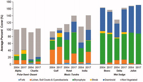
Table 6. Z-Statistics and p values for the Wilcoxon Signed-Rank Test.

	Wet Sedge (n = 12)		Mesic Tundra (n = 12)		Polar Semi-Desert (n = 8)
	Z	p (2-tailed)	Z	p (2-tailed)	Z	p (2-tailed)
Forb	−0.222^b	0.824	−0.314^b	0.754	−1.260^b	0.208
Lichen, Soil Crust & Cyanobacteria	−1.069^b	0.285	−2.981^b	0.003	−1.400^c	0.161
Bryophyte	−0.628^c	0.530	−0.314^b	0.754	−0.676^c	0.499
Shrub	−0.421^b	0.674	−2.371^b	0.018	−1.214^c	0.225
Graminoid	−1.767^b	0.077	−2.118^b	0.034	−2.028^c	0.043
Total Non-Vegetated	−0.800^c	0.424	−1.804^c	0.071	−0.420^b	0.674
Total Vegetated	−1.020^b	0.308	−1.255^c	0.209	0.000^d	1.000

Bold indicates significance at α = 0.05, superscript ^bbased on positive ranks, superscript ^cbased on negative ranks, superscript ^dthe sum of the negative ranks is equal to the sum of the positive rank.

As seen in Table 6, statistically significant (α = 0.05) increases in lichen, shrub and graminoid cover were observed for the mesic tundra. In the polar semi-desert, statistically significant decreases in graminoids were observed. No statistically significantly changes were observed in the wet sedge plots. The increase in the cover of lichen, soil crusts and cyanobacteria was statistically significant (Z = −2.981, p = 0.003) for the mesic tundra. As can be seen in Figure 3, this was most pronounced in the mesic tundra plots of India and Hotel. From the Braun-Blanquet field observations, this increase can largely be attributed to increases in the coverage of cyanobacteria (e.g., Nostoc commune) on top of the moss layer. In some quadrats in the 2017 observations, the cyanobacteria had dried, leaving a crusty, dark cover over the moss. In both Hotel and India, none of the Braun-Blanquet observations contained shrubs in 2004. However, in 2017, there were two observations of shrub in Hotel and one observation in India of Salix arctica (Arctic willow). This small, yet statistically significant (Z = −2.371, p = 0.018) increase, could be interpreted as an increase in shrub coverage in these mesic plots. However, due to the sparse Salix arctica observed in these plots, there is also the possibility it was present in 2004 but was omitted from random sampling. As portrayed in Figure 3, there was a small increase in graminoid cover in all mesic plots. This increase was considered statistically significant (Z = −2.118, p = 0.034). The total non-vegetated areas did not change significantly for any vegetation type.

NDVI Time Series Analysis: Vegetation Types

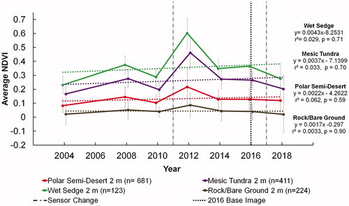
The NDVI time series for randomly selected pixels across the study area by vegetation type in the post-normalization images are illustrated in Figure 4. The rock/bare ground pixels (that are assumed to be unchanging over time) have a near-horizontal trend line. This demonstrates that the normalization procedure was successful in removing bias due to sensor and atmospheric differences between images. Further analysis about the performance of the normalization procedure can be found in the Supplemental Information. There are no significant trends in the normalized data for any of the vegetation types. As expected, the average NDVI was highest in the wetter vegetation communities, with wet sedge having the highest NDVI and PVC values in any given year, followed by mesic tundra and polar semi-desert.

Figure 4. NDVI over time for randomly selected pixels by vegetation cover type at 2 m spatial resolution with trend lines and standard deviation.

NDVI Time Series Analysis: ALDs

The 2 m and 30 m resolution NDVI time series for the toe, scar and entire ALD for Ptarmigan and Big Slide are presented in Figure 5 while ALD05 and ALD08 are presented in Figure 6. These ALDs occurred in the summer of 2007, so we would expect to see a change in NDVI between 2004 and 2008. At the 2 m resolution, the expected decrease in NDVI (due to the removal of vegetation) can be seen in all of the scar zones except for ALD08. For the toe where vegetation from upslope is deposited, the NDVI values increased in 2008 relative to 2004 (prior to disturbance). Similar to the findings of Rudy et al. (2013), the NDVI characteristics of the toe (i.e., area with some areas of intact vegetation) are similar to that of the surrounding undisturbed area.

Figure 5. Change in NDVI within active layer detachments (ALDs) at the Cape Bounty Arctic Watershed Observatory, Melville Island, Nunavut with NDVI plots for Ptarmigan and Big Slide at 2 and 30 m ‘upscaled’ resolution respectively. Error bars represent standard deviation. Graphs are overlaid over the 2012 NDVI image at 2 m resolution (left) and ‘upscaled’ 30 m resolution (right).

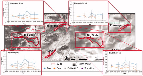
Figure 6. Change in NDVI within active layer detachments (ALDs) at the Cape Bounty Arctic Watershed Observatory, Melville Island, Nunavut with NDVI plots for ALD05 and ALD08 at 2 and 30 m ‘upscaled’ resolution respectively. Error bars represent standard deviation. Graphs are overlaid over the 2012 NDVI image at 2 m resolution (left) and ‘upscaled’ 30 m resolution (right).

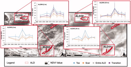
When the trends are compared to different spatial resolutions (i.e., 30 m spatial resolution in Figures 5 and 6), it was observed that the NDVI values for the toe and scar zones were not always distinguishable from each other in the ‘upscaled’ 30 m data. This is especially true for narrow ALDs (ALD05 and Ptarmigan). In these cases, the combination of the orientation of the ALD and coarser spatial resolution resulted in very few pixels being entirely contained within the confines of the ALD.

Discussion

Potential Influence of Image Acquisition Dates on NDVI Trends

It is important to demonstrate that the results observed here for high spatial resolution remote sensing data are not simply due to the timing of image acquisition (i.e., low NDVI values being a result of images acquired too early or too late in the growing season). In Figure 7a, the average NDVI for each vegetation type is plotted against the date of acquisition. If the timing of the image acquisition was impacting the analysis, we would expect to see low NDVI values at the earlier and later points of the season in relation to those collected in mid-season (i.e., time of ‘peak’ vegetation). With the exception of 2012 (which was a very warm year with an extended GSL; see Figure 2), all years occupy similar ranges of NDVI values. The lack of any trend suggests that the images were collected at comparable points in the growing season (i.e., close to peak vegetation productivity) and can be treated as similar to maximum NDVI. Though additional images within the growing season would likely add more nuance and clarity to the maximum NDVI (potentially by vegetation type), given that the growing season in the High Arctic is short and often cloudy, the lack of any trend in NDVI by day of acquisition within the growing season suggests that a single high spatial resolution optical data can be used with some level of confidence in a time series analysis. Similarly, Atkinson et al. (2020) found that NDVI derived from a single peak growing season IKONOS image could successfully model CO₂ exchange rates at landscape scales for the CBAWO.

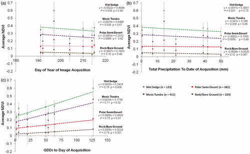
Figure 7. Average NDVI for randomly selected pixels (2 m) within vegetation cover types at the Cape Bounty Arctic Watershed Observatory, Melville Island, Nunavut plotted with standard deviation against: a) day of year of image acquisition; b) total precipitation to date of acquisition; and c) GDD₅ to date of acquisition.

Environmental Variables, PVC and Greenness

As expected, the NDVI values and PVC measurements of each vegetation type were related to moisture availability, with the highest NDVI values belonging to the wet sedge, followed by the mesic tundra (intermediate soil moisture) and polar semi-desert (Figures 3 and 4). Water availability is important for both vascular plants (i.e., shrubs, graminoids and forbs) (Bell and Bliss 1980; Klady et al. 2011) as well as bryophytes (May et al. 2018; Proctor 2007; Rixen and Mulder 2005). However, as can be observed in Figure 7b, there does not appear to be a clear linear relationship between the amount of precipitation received during the growing season prior to image acquisition and the NDVI value. This suggests that in this area, water from other sources (i.e., snow melt, water stored within the active layer) is more important than rainfall.

Substantial variation in the NDVI values was observed for the vegetation plots at the landscape scale (Figure 4) and for the ALDs (Figures 5 and 6) but there was no significant linear trend with time (Figure 4). A potential explanation is that despite there being a small statistically significant positive (p = 0.033) trend in the mean July temperatures from 1948–2017 at the nearest permanent weather station located in Mold Bay, NWT (Environment and Climate Change Canada 2018), there was no significant NDVI trend at the CBAWO from 2003–2018. This suggests that the trends in warming temperatures have not been sufficient (or persistent for a sufficiently long period) to result in a significant change in NDVI. This observation is consistent with the field PVC measurements. Significant increases in shrubs and graminoids were observed, but these were limited to the mesic tundra, and were small (Figure 3, Table 6). These results support the consensus that vegetation trends (i.e., greening and browning) in a warming Arctic are complex, highly variable and inherently scale-dependent (Myers-Smith et al. 2020). Here, environmental variables, specifically temperature in concert with moisture availability give rise to differing rates of greening at local scales.

When the average NDVI of the randomly selected pixels in each vegetation class is plotted against GDD₅ to image acquisition date, there is a strong linear relationship (Figure 7c) for the wet sedge (r² = .081, p = 0.006), mesic tundra (r²= 0.72, p = 0.016) and polar semi-desert (r²= 0.72, p = 0.011). This indicates that higher temperatures during the growing season contribute to enhanced greenness. When the strength of the relationships is considered, it is clear that the influence of increased temperature (i.e., steepness of the slope of the linear trend line) on the NDVI values was strongest for the wet sedge, with progressively shallower slopes for the mesic tundra and polar semi-desert areas. Here, we observed an increase in shrub cover in the mesic plots at the CBAWO between 2004 and 2017. With research suggesting that moisture availability increases the potential growth of Arctic shrubs under warming conditions (e.g., Ackerman et al. 2017; Arruda 2016; Klady et al. 2011), our findings suggest that with available moisture, continued warming may increase shrub growth in the mesic tundra.

Additionally, the weakening relationship and shallower slope in the drier vegetation types (Figure 7c) may be explained by two factors. First, there is simply less vegetation present per unit area than in the wet sedge areas. Thus, increases in NDVI from increased vegetation productivity of existing plants (e.g., increased leaf growth) may be dampened by the lack of response from the rock/bare soil fraction. Second, as the vegetation communities are only found in areas where there is also sufficient water, increases in temperature alone may not increase vegetation cover. Thus, the vegetation response to warming may be low due to other limiting factors (e.g., moisture and nutrient availability).

Potential Long-Term Impacts of Extreme Warming

The years 2007 and 2012 were exceptionally warm years in the circumpolar region and at the CBAWO. Sea ice extent reached a record minimum in September 2007 (Stroeve et al. 2008) only to have a new record minimum set in 2012 (Kirchmeier-Young et al. 2017; National Snow and Ice Data Center 2018). At the CBAWO, the warming events of 2007 caused the initiation of numerous ALDs across the study area (Lamoureux and Lafrenière 2009). As shown in our study, the scar zones of these disturbed areas remain largely non-vegetated. Research in other disturbed areas suggests that these scar zones will take several decades to reach a similar vegetation cover, and potentially even longer to reach a similar biological diversity as the surrounding undisturbed area (Cannone et al. 2010). As illustrated in Figure 2, the number of GDD₅ accumulated in 2012 was more than double those accumulated for any other year. In their 2018 report on climate change, Environment and Climate Change Canada found that from 1948–2016, northern Canada (here, defined as the three northern territories; Yukon, Northwest and Nunavut) experienced an increase of 2.3 °C, 1.6 °C and 4.3 °C in the annual, summer and winter mean temperatures respectively (Zhang et al. 2019). In addition to changes in mean temperature, changes in the extreme minimum and maximum temperatures have been reported (Vincent et al. 2012) and are forecasted to continue to increase (Zhang et al. 2019).

As demonstrated in Figure 7c and discussed above, there is a strong relationship between GDD₅ (a function of temperature) and observed NDVI. The warm summer of 2012 resulted in higher NDVI values with greener vegetation. If changes in climate result in more years like 2012, it is anticipated that there will be enhanced ecosystem productivity and perhaps impacts on biodiversity. The lower NDVI values in the following years suggest that it is possible that some of the new growth that was initiated in the very warm summer of 2012 did not experience green up in the following summers. This suggests that these shoots may have added to the amount of senesced (i.e., non-photosynthetic) vegetation present on the landscape. This non-photosynthetic vegetation is not characterized by NDVI, but has been shown to be modeled by other remote sensing data including hyperspectral (Li and Guo 2018), LiDAR (light detection and ranging) and synthetic aperture radar (SAR) (reviewed in Li and Guo 2016) in temperate ecosystems. A vegetation index similar to NDVI, but using the NIR and green bands of WorldView-2 has been shown to model the fraction of absorbed photosynthetically active radiation in a temperate wetland, which partially accounts for the presence of senesced vegetation (Schile et al. 2013). There appears to be a data gap for modeling senesced vegetation in High Arctic systems, and the application of indices that better account for senesced vegetation may be a useful area for future analysis of change. The increased growth in 2012 that did not green up the following year may have resulted in increased litter availability. Given decay rates are slow in this region (Hobbie 1996), there may be lag effects of highly productive years on the nutrient cycling of the ecosystems in following years. Additionally, if warming results in greater growth in shrub species that have a higher attribution of carbon to woody stems, the slower decomposition rates associated with these species may have a minor impact on the long-term carbon storage of these systems.

Active Layer Detachments

Though the results of the 2 m data and the ‘upscaled’ 30 m data were similar at the landscape level (results not presented here), the results differed for the analysis of the ALDs. Of the large ALDs examined in this study, the 30 m analysis was not always able to distinguish between the different areas (i.e., toe versus scar, or areas of transition) within the ALDs (Figures 5 and 6). The ALDs are often less than a pixel wide in the ‘upscaled’ analysis (i.e., 30 m spatial resolution). As only the largest of the ALDs in the study area were selected for analysis, it is likely that this discrepancy would become more apparent as ALDs approach Landsat pixel and sub-pixel scales. It is important to understand how scar zones of ALDs are stabilizing and revegetating as it has been shown that these disturbed areas can serve as a source of labile organic matter (Grewer et al. 2015) which can have impacts on biogeochemical cycling downstream. Additionally, the scar zones have been shown to have different ecosystem exchange and respiration rates than the surrounding undisturbed areas (Beamish et al. 2014). As permafrost disturbances become more widespread in the High Arctic, tracking them, regardless of size, may help inform carbon sequestration and release models (e.g., Atkinson et al. 2020).

Studies that have examined Landsat data to describe land cover and predict changes due to a modified climate in the Arctic have found that the application of higher spatial resolution imagery (aerial or satellite) improved their analyses (Lara et al. 2018; Zhang et al. 2013); i.e., high spatial resolution data are able to measure the less dominant land cover classes and capture more variation on the landscape (Hung and Treitz 2020). Thus, if features like permafrost disturbances that are locally significant but cover small areas are to be included in the analysis, the inclusion of high spatial resolution data is important.

Arctic Vegetation Change Observed at Different Scales

To quantify vegetation change at the circumpolar level, many studies have used products with a high temporal resolution, but low spatial resolution (i.e., AVHRR/GIMMS). These studies have observed greening trends in the Svalbard area (Vickers et al. 2016), the Siberian Arctic (Dutrieux et al. 2012) and the entire circumpolar region (Bhatt et al. 2013) over the past few decades. These studies have also shown a tendency for browning to occur in some regions in the later part of the time series analysis, despite the continued rise in Arctic temperatures. Though changes to large-scale atmospheric patterns resulting in increased cloudiness have been suggested (Dutrieux et al. 2012; Bhatt et al. 2013), there have also been calls to determine what factors are responsible for these changes at the plot level (Pattison et al. 2015).

There have also been calls to further evaluate NDVI time series against field measurements in order to resolve differences between different remote sensing products (Guay et al. 2014; Pattison et al. 2015). Comparisons of different NDVI time series for the Arctic have shown inconsistencies, highlighting the challenges associated with comparing results from sensors with different bandwidths, spatial resolutions and calibration settings (Guay et al. 2014). However, as the results from studies using different remote sensing products are used to understand changes in biophysical properties of vegetation and improve model development, it is important to understand how the results of analyses performed with different sensors relates to processes on the ground. Separate from combining images from different sensors to construct a single time series (as was done in this study), it has been found that in some areas, the NDVI trends observed in the 8 km resolution GIMMS dataset do not correspond with observations on the ground or with those observed with Landsat data and ground observations (Raynolds et al. 2013; Pattison et al. 2015; Ju and Masek 2016). This raises the question of what may be causing the discrepancies between analyses performed with different satellite products. Here, the size of the study area (approximately 100 km²) would make comparisons to the GIMMS dataset impractical, as the entire study area would only be covered by a few pixels. Though cloud free image availability within the short growing season does pose a challenge, comparisons to sensors like Landsat with a 30 m spatial resolution are more feasible when scale alone is considered.

Ideally, to properly compare 2 m and 30 m datasets, Landsat data for each of the corresponding years would be compared to the aggregated high spatial resolution data (i.e., originating from IKONOS, WorldView-2 and WorldView-3). Edwards and Treitz (2017) completed a time series analysis of the CBAWO using Landsat TM and OLI data from 1985 to 2015. Unfortunately, the images used by Edwards and Treitz (2017) were acquired during years when cloud-free high spatial resolution data were not available, thereby limiting our ability to perform a year-to-year comparison. Additionally, given the time frames for the two studies are very different (i.e., 30 versus 14 years), caution should be applied when comparing overall trends. For instance, in the current analysis, 2012 was an especially warm year with high NDVI values that had a strong influence on the trend. However, Landsat data were not available for the CBAWO in 2012 (Edwards and Treitz 2017). Though the error associated with different times of acquisition within the growing season is generally considered to be random and can generally be ignored within a given time series (e.g., Ju and Masek 2016) (Figure 2), it is not clear if the same can be said when comparing different time series. When comparing the findings of times series analysis that use coarser spatial resolution products to those based on high and moderate spatial resolution data that tend to have fewer observations, the inclusion or exclusion of very warm years like 2012 may significantly alter the outcome (i.e., result in the time series being significant or not as illustrated in Figure 4. Although there is no correlation between the date of acquisition and the average NDVI value for all plots, 2012 remains an outlier. Thus, the potential lack of data for extreme years may contribute to the discrepancies between time series produced with products with different temporal resolutions.

Benefits and Challenges of Using High Spatial Resolution Data from Multiple Sensors

High spatial resolution remote sensing data capture substantial variability on the landscape (i.e., more precise conditions). In this study, 2 m data were found to be capable of delineating the different components of ALDs in a way that ‘upscaled’ 30 m data could not. However, using high spatial resolution data in the Arctic has challenges. The length of the data record is rather short compared to many of the coarser resolution products, given these data are tasked for specific coverages rather than collected automatically/routinely. To have access to 15 years of high spatial resolution remote sensing data for a site in the Canadian High Arctic is unique, albeit from three different sensors (i.e., IKONOS and WorldView-2, WorldView-3). Since most high spatial resolution satellites were launched in the late 1990s and early 2000s, there is a limited depth of historical imagery compared to intermediate and coarser spatial resolution products, particularly for large areas at high latitudes. For a terrestrial system that changes slowly, this compressed time series limits the capacity for examining incremental environmental change, specifically vegetation where the growing season is limited.

Although rapid improvements in remote sensing technology can improve research outcomes, having multiple commercial sensors creates challenges for calibrating one sensor to another. For example, in this study, IKONOS, WorldView-2, and WorldView-3 data were used. There was only a 5-year period where IKONOS and WorldView-2 (2009–2015) were in orbit simultaneously. The short overlap time, the length of the tasking window, the short growing season, the high probability of cloud cover, and the high cost of acquiring high spatial resolution imagery rendered it impractical to acquire data from both sensors at this site in a given year. In comparison, the sensor design and launch of new sensors in other satellite missions (e.g., Landsat series, AVHRR) is conducted with continuity of missions being of paramount importance.

To maximize the utility of high spatial resolution imagery, each scene must be properly aligned so that each pixel in the image stack is properly co-registered. To best achieve this, the user must have access to a high-quality DEM and accurate and precise GCPs. With the recent release of the 2-m Arctic DEM for the circumpolar region produced by the Polar Geospatial Center, researchers without access to stereo-pair imagery for their study area may still be able to perform accurate geometric corrections. However, the collection of GCPs needed for orthorectification and image registration processes may still pose a challenge. As there are few permanent anthropogenic structures on the Arctic landscape, researchers must either install their own targets or attempt to find naturally occurring features that are visible in the imagery and that remain in the same position each year. In this setting, the natural features that best approach this requirement are rivers, lakes and ocean coast lines. However, these features are not always stable over time. For example, due to the braided nature of many of the rivers, the exact location of the main channel may change (on the order of metres) from year to year. Additionally, changes in ice cover on lakes sometimes obscures the true edge of the lake shore. This presented a challenge for performing a geometric correction to the IKONOS 2004 data as the installation of tarps and corner reflectors occurred at a later date. For some studies, this may complicate the utility of incorporating historical data into time series analyses.

The PIF method was chosen to normalize the images in this study due to its ability to account for a variety of factors in an Arctic setting without access to empirical atmospheric data. Selecting PIFs in this environment was an iterative process resulting in a different set of dark PIFs for each image date. Furthermore, it was found that the normalization regression equations were heavily dependent on the presence or absence of dark PIFs. As it is not a guarantee that there will ice free waters available for dark PIF selection at these high latitudes and not all areas of interest include large bodies of water, the PIF method may be limited in its applicability in an Arctic setting where the most reliable targets are limited to the brighter reflectance surfaces (i.e., bedrock and dry bare soil).

Additionally, this method normalizes each band separately. Though this is a common technique in other ecological systems and has been used in the Arctic (e.g., Edwards and Treitz 2017; Bonney et al. 2018), some suggest that normalizing each band individually may result in unexpected discrepancies (Syariz et al. 2019). This study used a spectral index (i.e., NDVI - a ratio between the red and NIR bands) to examine terrestrial ecosystem change. However, if the normalization behaved differently for the red and NIR bands, the resulting NDVI value may be biased.

Conclusions

In this study, high spatial resolution data from IKONOS, WorldView-2 and WorldView-3 (2004–2018) were examined in concert with field measurements to investigate changes in vegetation at a Canadian High Arctic site. The PIF method was applied to normalize data collected by these high spatial resolution sensors. Field observations exhibited small, but statistically significant increases in shrubs and graminoids in the mesic tundra between 2004 and 2017. However, no significant change in total vegetation cover was observed in the field. Likewise, NDVI did not exhibit a statistically significant change during this period, but there was a statistically significant relationship between NDVI and GDD₅ for all vegetation types. The results indicate that higher temperatures result in higher NDVI values. In addition, as the Artic warms, there will likely be an increase in permafrost disturbances which can have local effects on vegetation cover lasting decades. While high spatial resolution data are well suited to tracking changes on the landscape, their utility is highlighted when identifying disturbances and tracking their recovery on the landscape.

Acknowledgements

The authors are grateful for the comments from the anonymous reviewers.

Additional information

Funding

This research was possible with the financial support from the Natural Sciences and Engineering Research Council (NSERC) and the Northern Scientific Training Program (NSTP) with logistical support from the Polar Continental Shelf Program (PCSP), Natural Resources Canada. The principal author gratefully acknowledges financial support from the Government of Ontario (Ontario Graduate Scholarship), NSERC (Canadian Graduate Scholarships-Masters) and Queen’s University (Tri-Agency Recipient Recognition Award).

References

- Ackerman, D., Griffin, D., Hobbie, S.E., and Finlay, J.C. 2017. “Arctic shrub growth trajectories differ across soil moisture levels.” Global Change Biology, Vol. 23(No. 10): pp. 4294–4302. doi:10.1111/gcb.13677.
- AMAP. 2019. “AMAP climate change update 2019: An update to key findings of Snow, Water, Ice and Permafrost in the Arctic (SWIPA) 2017.” Arctic Monitoring and Assessment Programme (AMAP), Oslo, Norway. 12 pp.
- Arruda, A. 2016. Impacts of enhanced temperature and snow deposition of senescence date, vegetation cover, and CO2 exchange in a Canadian High Arctic mesic ecosystem. MSc dissertation. Kingston, ON: Queen's University.
- Atkinson, D.M., and Treitz, P. 2012. “Arctic ecological classifications derived from vegetation community and satellite spectral data.” Remote Sensing, Vol. 4 (No. 12): pp. 3948–3971. doi:10.3390/rs4123948.
- Atkinson, D.M., and Treitz, P. 2013. “Modeling biophysical variables across an Arctic latitudinal gradient using high spatial resolution remote sensing data.” Arctic Antarctic and Alpine Research, Vol. 45(No. 2): pp. 161–178. doi:10.1657/1938-4246-45.2.161.
- Atkinson, D.M., Hung, J.K.Y., Gregory, F., Scott, N., and Treitz, P. 2020. “High spatial resolution remote sensing models for landscape-scale CO# exchange in the Canadian Arctic.” Arctic, Antarctic, and Alpine Research, Vol. 52(No. 1): pp. 248–263. doi:10.1080/15230430.2020.1750805.
- Barrett, R.T., and Hollister, R.D. 2016. “Arctic plants are capable of sustained responses to long-term warming.” Polar Research, Vol. 35 (No. 1): pp. 25405–25409. (2016):doi:10.3402/polar.v35.25405.
- Barrett, R.T.S., Hollister, R.D., Oberbauer, S.F., and Tweedie, C.E. 2015. “Arctic plant responses to changing abiotic factors in northern Alaska.” American Journal of Botany, Vol. 102(No. 12): pp. 2020–2031. doi:10.3732/ajb.1400535.
- Beamish, A., Neil, A., Wagner, I., and Scott, N.A. 2014. “Short-term impacts of active layer detachments on carbon exchange in a High Arctic ecosystem, Cape Bounty.” Polar Biology, Vol. 37 (No. 10): pp. 1459–1468. doi:10.1007/s00300-014-1536-4.
- Beel, C.R., Lamoureux, S.F., and Orwin, J.F. 2018. “Fluvial response to a period of hydrometeorological change and landscape disturbance in the Canadian High Arctic.” Geophysical Research Letters, Vol. 45 (No. 19): pp. 10,446–10455. doi:10.1029/2018GL079660.
- Bell, K., and Bliss, L. 1980. “Plant Reproduction in a High Arctic Environment.” Arctic and Alpine Research, Vol. 12(No. 1): pp. 1–10. doi:10.2307/1550585.
- Bhatt, U., Walker, D., Raynolds, M., Bieniek, P., Epstein, H., Comiso, J., Pinzon, J., Tucker, C., and Polyakov, I. 2013. “Recent Declines in Warming and Vegetation Greening Trends over Pan-Arctic Tundra.” Remote Sensing, Vol. 5(No. 9): pp. 4229–4254. doi:10.3390/rs5094229.
- Bhatt, U.S., Walker, D.A., Raynolds, M.K., Bieniek, P.A., Epstein, H.E., Comiso, J.C., Pinzon, J.E., et al. 2017. “Changing seasonality of panarctic tundra vegetation in relationship to climatic variables.” Environmental Research Letters, Vol. 12(No. 5): pp. 055003. doi:10.1088/1748-9326/aa6b0b.
- Bjorkman, A.D., Criado, M.G., Myers-Smith, I.H., Ravolainen, V., Jónsdóttir, I.S., Westergaard, K.B., Lawler, J.P., et al. 2020. “Status and trends in Arctic vegetation: Evidence from experimental warming and long-term monitoring.” Ambio, Vol. 49 (No. 3): pp. 678–692. doi:10.1007/s13280-019-01161-6.
- Bonney, M.T., Danby, R.K., and Treitz, P.M. 2018. “Landscape variability of vegetation change across the forest to tundra transition of central Canada.” Remote Sensing of Environment, Vol. 217 pp. 18–29. doi:10.1016/j.rse.2018.08.002.
- Braun-Blanquet, J. 1932. Plant Sociology: The Study of Plant Communities. Authorized English translation of Planzensoziologie. Translated, revised and edited by G.D. Fuller and H.S. Conard. New York, NY. McGraw Hill.
- Braun-Blanquet, J. 1946. “Ṻber den Deckungswert der Arten in den Pflanzengesellschaften der Ordnung Vaccinio-Piceetalia.” Jahresber. Naturforsch. Ges. Graubfindens, Vol. 130: pp. 119.
- Braun-Blanquet, J. 1965. Plant Sociology: The Study of Plant Communities. Translated, revived, and edited by C.D. Fuller and H.S. Conard, 439. London: Hafner.
- Cannone, N., Lewkowicz, A.G., and Guglielmin, M. 2010. “Vegetation colonization of permafrost-related landslides, Ellesmere Island, Canadian high arctic.” Journal of Geophysical Research, Vol. 115 (No. G4): pp. 1–10. doi:10.1029/2010JG001384.
- Carter, T. 1998. “Changes in the thermal growing season in Nordic countries during the past century and prospects for the future.” Agricultural and Food Science, Vol. 7 (No. 2): pp. 161–179. doi:10.23986/afsci.72857.
- Chen, X., Vierling, L., and Deering, D. 2005. “A simple and effective radiometric correction method to improve landscape change detection across sensors and across time.” Remote Sensing of Environment, Vol. 98 (No. 1): pp. 63–79. doi:10.1016/j.rse.2005.05.021.
- Damgaard, C. 2014. “Estimating mean plant cover from different types of cover data: A coherent statistical framework.” Ecosphere, Vol. 5(No. 2): pp. art20. doi:10.1890/ES13-00300.1.
- Davis, E., Trant, A., Hermanutz, L., Way, R.G., Lewkowicz, A.G., Collier, L.S., Currier, A., and Whitaker, D. 2020. “Plant-environment interactions in the low arctic torngat mountains of labrador.” Ecosystems. doi:10.1007/s10021-020-00577-6.
- Dorigo, W.A., Zurita-Milla, R., de Wit, A.J.W., Brazile, J., Singh, R., and Schaepman, M.E. 2007. “A review on reflective remote sensing and data assimilation techniques for enhanced agroecosystem modeling.” International Journal of Applied Earth Observation and Geoinformation, Vol. 9(No. 2): pp. 165–193. doi:10.1016/j.jag.2006.05.003.
- Dutrieux, L.P., Bartholomeus, H., Herold, M., and Verbesselt, J. 2012. “Relationships between declining summer sea ice, increasing temperatures and changing vegetation in the Siberian Arctic tundra from MODIS time series (2000 – 11.” Environmental Research Letters, Vol. 7 (No. 4): pp. 044028–044012. doi:10.1088/1748-9326/7/4/044028.
- Eckhardt, D.W., Verdin, J.P., and Lyford, G.R. 1990. “Automated Update of an Irrigated Lands GIs Using SPOT HRV Imagery.” Photogrammetric Engineering and Remote Sensing, Vol. 56(No. 11): pp. 1515–1522.
- Edwards, M., and Henry, G.H.R. 2016. “The effects of long-term experimental warming on the structure of three High Arctic plant communities.” Journal of Vegetation Science, Vol. 27 (No. 5): pp. 904–910. doi:10.1111/jvs.12417.
- Edwards, R., and Treitz, P. 2017. “Vegetation greening trends at two sites in the Canadian Arctic: 1984–2015.” Arctic, Antarctic, and Alpine Research, Vol. 49(No. 4): pp. 601–619. doi:10.1657/AAAR0016-075.
- Elmendorf, S.C., Henry, G.H., Hollister, R.D., Björk, R.G., Bjorkman, A.D., Callaghan, T.V., Collier, L.S., et al. 2012. “Global assessment of experimental climate warming on tundra vegetation: Heterogeneity over space and time.” Ecology Letters, Vol. 15 (No. 2): pp. 164–175. doi:10.1111/j.1461-0248.2011.01716.x.
- Environment and Climate Change Canada. 2018. “Adjusted and homogenized Canadian Climate data.” Environment and Climate Change Canada, last assessed November 2018, https://www.canada.ca/en/environment-climate-change/services/climate-change/science-research-data/climate-trends-variability/adjusted-homogenized-canadian-data/surface-air-temperature.html
- Epstein, H., Bhatt, U., Raynolds, M., Walker, D., Forbes, B., Phoenix, G., Bjerke, J., et al. 2018. “Vital Signs: Tundra Greenness. Arctic Report Card: Update for 2018.” NOAA, last accessed November 2018, https://www.arctic.noaa.gov/Report-Card/Report-Card-2018/ArtMID/7878/ArticleID/777/Tundra-Greenness
- Epstein, H., Raynolds, M., Walker, D., Bhatt, U., Tucker, C., and Pinzon, J. 2012. “Dynamics of aboveground phytomass of the circumpolar Arctic during the past three decades.” Environmental Research Letters, Vol. 7 (No. 1): pp. 015506. doi:10.1088/1748-9326/7/1/015506.
- Fleming, D. 2001. “Ikonos DN value conversion to planetary reflectance values.” CRESS Project: UMCP Geography, pp. 1–4. http://web.unicen.edu.ar/crecic/docs/radrefl.pdf
- Fraser, R.H., Lantz, T.C., Olthof, I., Kokelj, S.V., and Sims, R.A. 2014. “Warming-Induced Shrub Expansion and Lichen Decline in the Western Canadian Arctic.” Ecosystems, Vol. 17 (No. 7): pp. 1151–1168. doi:10.1007/s10021-014-9783-3.
- Freemantle, V. A. 2019. A high spatial resolution satellite remote sensing time series analysis of Cape Bounty, Melville Island, Nunavut (2004–2018). MSc Thesis. Kingston, Ontario, Canada: Department of Geography and Planning, Queen’s University.
- Furman, B.T., Leone, E.H., Bell, S.S., Durako, M.J., and Hall, M.O. 2018. “Braun-Blanquet data in ANOVA designs: Comparisons with percent cover and transformations using simulated data.” Marine Ecology Progress Series, Vol. 597: pp. 13–22. doi:10.3354/meps12604.
- Garcia-Torres, L., Caballero-Novella, J., Gomez-Candon, D., and De-Castro, A. 2014. “Semi-Automatic Normalization of Multitemporal Remote Images Based on Vegetative Pseudo-Invariant Features.” PLOS One, Vol. 9(No. 3): pp. e91275. doi:10.1371/journal.pone.0091275.
- Gregory, F. M. 2011. Biophysical remote sensing and terrestrial CO2 exchange at Cape Bounty, Melville Island. MSc Thesis. Kingston, Ontario, Canada: Department of Geography and Planning, Queen’s University.
- Grewer, D.M., Lafrenière, M.J., Lamoureux, S.F., and Simpson, M.J. 2015. “Potential shifts in Canadian High Arctic sedimentary organic matter composition with permafrost active layer detachments.” Organic Geochemistry, Vol. 79: pp. 1–13. doi:10.1016/j.orggeochem.2014.11.007.
- Guay, K.C., Beck, P.S.A., Berner, L.T., Goetz, S.J., Baccini, A., and Buermann, W. 2014. “Vegetation productivity patterns at high northern latitudes: A multi-sensor satellite data assessment.” Global Change Biology, Vol. 20(No. 10): pp. 3147–3158. doi:10.1111/gcb.12647.
- Haboudane, D., Miller, J.R., Tremblay, N., Zarco-Tejada, P.J., and Dextraze, L. 2002. “Integrated narrow-band vegetation indices for prediction of crop chlorophyll content for application to precision agriculture.” Remote Sensing of Environment, Vol. 81(No. 2–3): pp. 416–426. doi:10.1016/S0034-4257(02)00018-4.
- Hakes, W. 1994. “On the predictive power of numerical and Braun-Blanquet classification: An example from beechwoods.” Journal of Vegetation Science, Vol. 5 (No. 2): pp. 153–160. doi:10.2307/3236147.
- Heo, J., and FitzHugh, T. 2000. “A standardized radiometric normalization method for change detection using remotely sensed imagery.” Photogrammetric Engineering and Remote Sensing, Vol. 66(No. 2): pp. 173–181.
- Hill, G.B., and Henry, G.H.R. 2011. “Responses of High Arctic wet sedge tundra to climate warming since 1980.” Global Change Biology, Vol. 17(No. 1): pp. 276–287. doi:10.1111/j.1365-2486.2010.02244.x.
- Hobbie, S. 1996. “Temperature and plant species control over litter decomposition in Alaskan tundra.” Ecological Monographs, Vol. 66(No. 4): pp. 503–522. doi:10.2307/2963492.
- Hong, G., and Zhang, Y. 2008. “A comparative study on radiometric normalization using high resolution satellite images.” International Journal of Remote Sensing, Vol. 29(No. 2): pp. 425–438. doi:10.1080/01431160601086019.
- Hope, A., Tague, C., and Clark, R. 2007. “Characterizing post ‐ fire vegetation recovery of California chaparral using TM / ETM + time ‐ series data.” International Journal of Remote Sensing, Vol. 28(No. 6): pp. 1339–1354. doi:10.1080/01431160600908924.
- Hudson, J., and Henry, G. 2009. “Increased plant biomass in a high arctic heath community from 1981 to 2008.” Ecology, Vol. 90(No. 10): pp. 2657–2663. doi:10.1890/09-0102.1.
- Hung, J.K.Y., and Treitz, P.M. 2020. “Environmental land-cover classification for integrated watershed studies: Cape Bounty, Melville Island, Nunavut.” Arctic Science, Vol. 6(No. 4): pp. 404–422. doi:10.1139/as-2019-0029.
- IPCC. 2018. Summary for policymakers. In: Global Warming of 1.5 °C. An IPCC Special Report on the Impacts of Global Warming of 1.5 °C Above Pre-Industrial Levels and Related Global Greenhouse Gas Emission Pathways, in the Context of Strengthening the Global Response to the Threat of Climate Change, Sustainable Development, and Efforts to Eradicate Poverty, edited by V. Masson-Delmotte, P. Zhai, H.O. Pörtner, D. Roberts, J. Skea, P.R. Shukla, A. Pirani, W. Moufouma-Okia, C. Péan, R. Pidcock, S. Connors, J.B.R. Matthews, Y. Chen, X. Zhou, M.I. Gomis, E. Lonnoy, T. Maycock, M. Tignor, T. Waterfield, 32. Geneva, Switzerland: World Meteorological Organization.
- Jensen, J. 2016. Introductory Digital Image Processing: A Remote Sensing Perspective. 4th ed. New Jersey, USA: Pearson Education Inc.
- Ju, J., and Masek, J.G. 2016. “The vegetation greenness trend in Canada and US Alaska from 1984–2012 Landsat data.” Remote Sensing of Environment, Vol. 176 pp. 1–16. doi:10.1016/j.rse.2016.01.001.
- Juszak, I., Erb, A.M., Maximov, T.C., and Schaepman-Strub, G. 2014. “Arctic shrub effects on NDVI, summer albedo and soil shading.” Remote Sensing of Environment, Vol. 153 pp. 79–89. doi:10.1016/j.rse.2014.07.021.
- Juszak, I., Eugster, W., Heijmans, M.M.P.D., and Schaepman-Strub, G. 2016. “Contrasting radiation and soil heat fluxes in Arctic shrub and wet sedge tundra.” Biogeosciences, Vol. 13(No. 13): pp. 4049–4064. doi:10.5194/bg-13-4049-2016.
- Kapfer, J., Virtanen, R., and Grytnes, J.A. 2012. “Changes in arctic vegetation on Jan Mayen Island over 19 and 80 years.” Journal of Vegetation Science, Vol. 23(No. 4): pp. 771–781. doi:10.1111/j.1654-1103.2012.01395.x.
- Karlsen, S.R., Anderson, H.B., Van Der Wal, R., and Hansen, B.B. 2018. “A new NDVI measure that overcomes data sparsity in cloud-covered regions predicts annual variation in ground-based estimates of high arctic plant productivity.” Environmental Research Letters, Vol. 13 (No. 2): pp. 025011. doi:10.1088/1748-9326/aa9f75.
- Kirchmeier-Young, M.C., Zwiers, F.W., and Gillett, N.P. 2017. “Attribution of extreme events in Arctic sea ice extent.” Journal of Climate, Vol. 30 (No. 2): pp. 553–571. doi:10.1175/JCLI-D-16-0412.1.
- Klady, R.A., Henry, G.H.R., and Lemay, V. 2011. “Changes in high arctic tundra plant reproduction in response to long-term experimental warming.” Global Change Biology, Vol. 17(No. 4): pp. 1611–1624. doi:10.1111/j.1365-2486.2010.02319.x.
- Kuester, M. 2016. “Radiometric use of WorldView-3 imagery.” DigitalGlobe, last accessed April 2018, https://dg-cms-uploads-production.s3.amazonaws.com/uploads/document/file/207/Radiometric_Use_of_WorldView-3_v2.pdf
- Kuester, M. 2017. “Absolute radiometric calibration: 2016v0.” DigitalGlobe, last accessed April 2018, https://dg-cms-uploads-production.s3.amazonaws.com/uploads/document/file/209/ABSRADCAL_FLEET_2016v0_Rel20170606.pdf
- Laidler, G.J., Treitz, P.M., and Atkinson, D.M. 2009. “Remote sensing of Arctic vegetation: Relations between the NDVI, spatial resolution and vegetation cover on Boothia Peninsula, Nunavut.” ARCTIC, Vol. 61(No. 1): pp. 1–13. doi:10.14430/arctic2.
- Lamoureux, S.F., and Lafrenière, M. 2009. “Fluvial impact of extensive active layer detachments. Cape Bounty, Melville Island, Canada.” Arctic, Antarctic, and Alpine Research, Vol. 41 (No. 1): pp. 59–68. doi:10.1657/1523-0430-41.1.59.
- Lara, M.J., Nitze, I., Grosse, G., Martin, P., and David McGuire, A. 2018. “Reduced arctic tundra productivity linked with landform and climate change interactions.” Scientific Reports, Vol. 8(No. 1): pp. 1–10. doi:10.1038/s41598-018-20692-8.
- Laurent, V.C.E., Verhoef, W., Clevers, J.G.P.W., and Schaepman, M.E. 2011. “Estimating forest variables from top-of-atmosphere radiance satellite measurements using coupled radiative transfer models.” Remote Sensing of Environment, Vol. 115(No. 4): pp. 1043–1052. doi:10.1016/j.rse.2010.12.009.
- Leffler, A.J., Klein, E.S., Oberbauer, S.F., and Welker, J.M. 2016. “Coupled long-term summer warming and deeper snow alters species composition and stimulates gross primary productivity in tussock tundra.” Oecologia, Vol. 181(No. 1): pp. 287–297. doi:10.1007/s00442-015-3543-8.
- Lewkowicz, A.G. 2007. “Dynamics of active-layer detachment failures, Fosheim Peninsula, Ellesmere Island, Nunavut, Canada.” Permafrost and Periglacial Processes, Vol. 18 (No. 1): pp. 89–103. doi:10.1002/ppp.578.
- Li, Z., and Guo, X. 2016. “Remote sensing of terrestrial non-photosynthetic vegetation using hyperspectral, multispectral, SAR, and LiDAR data.” Progress in Physical Geography: Earth and Environment, Vol. 40(No. 2): pp. 276–304. doi:10.1177/0309133315582005.
- Li, Z., and Guo, X. 2018. “Non-photosynthetic vegetation biomass estimation in semiarid Canadian mixed grasslands using ground hyperspectral data, Landsat 8 OLI, and Sentinel-2 images.” International Journal of Remote Sensing, Vol. 39(No. 20): pp. 6893–6913. doi:10.1080/01431161.2018.1468105.
- May, J.L., Parker, T., Unger, S., and Oberbauer, S.F. 2018. “Short term changes in moisture content drive strong changes in Normalized Difference Vegetation Index and gross primary productivity in four Arctic moss communities.” Remote Sensing of Environment, Vol. 212 pp. 114–120. doi:10.1016/j.rse.2018.04.041.
- McNellie, M.J., Dorrough, J., and Oliver, I. 2019. “ Species abundance distributions should underpin ordinal cover-abundance transformation.” Applied Vegetation Science, Vol. 22 pp. 361–372.
- Myers-Smith, I.H., Forbes, B.C., Wilmking, M., Hallinger, M., Lantz, T., Blok, D., Tape, K., et al. 2011. “Shrub expansion in tundra ecosystems: Dynamics, impacts and research priorities.” Environmental Research Letters, Vol. 6(No. 4): pp. 045509. doi:10.1088/1748-9326/6/4/045509.
- Myers-Smith, I.H., Kerby, J.T., Phoenix, G.K., Bjerke, J.W., Epstein, H.E., Assmann, J.J., John, C., et al. 2020. “Complexity revealed in the greening of the Arctic.” Nature Climate Change, Vol. 10 (No. 2): pp. 106–117. doi:10.1038/s41558-019-0688-1.
- NASA. n.d. “Landsat 7 Science Data Users Handbook.” Last accessed January 2017, http://ltpwww.gsfc.nasa.gov/IAS/handbook/handbook_htmls/chapter12/chapter12.html
- National Snow and Ice Data Center. 2018. “Arctic sea ice extent arrives at its minimum.” Last accessed online April 29, 2019, https://nsidc.org/arcticseaicenews/2018/09/arctic-sea-ice-extent-arrives-at-its-minimum/
- Overland, J.E., Wang, M., Walsh, J.E., and Stroeve, J.C. 2014. “Future Arctic climate changes: Adaptation and mitigation time scales.” Earth's Future, Vol. 2 (No. 2): pp. 68–74. doi:10.1002/2013EF000162.
- Pattison, R.R., Jorgenson, J.C., Raynolds, M.K., and Welker, J.M. 2015. “Trends in NDVI and Tundra community composition in the Arctic of NE Alaska between1984 and 2009.” Ecosystems, Vol. 18(No. 4): pp. 707–719. doi:10.1007/s10021-015-9858-9.
- Proctor, M.C., Oliver, M.J., Wood, A.J., Alpert, P., Stark, L.R., Cleavitt, N.L., and Mishler, B.D. 2007. “Desiccation-tolerance in bryophytes: A review.” Bryologist, Vol. 110(No. 4): pp. 595–621. doi:10.1639/0007-2745(2007)110[595:DIBAR]2.0.CO;2.
- Raynolds, M.K., and Walker, D.A. 2016. “Increased wetness confounds Landsat-derived NDVI trends in the central Alaska North Slope region, 1985–2011.” Environmental Research Letters, Vol. 11(No. 8): pp. 085004–085013. doi:10.1088/1748-9326/11/8/085004.
- Raynolds, M.K., Walker, D.A., Verbyla, D., and Munger, C.A. 2013. “Patterns of change within a tundra landscape: 22-year Landsat NDVI trends in an area of the northern foothills of the Brooks Range, Alaska.” Arctic, Antarctic, and Alpine Research, Vol. 45(No. 2): pp. 249–260. doi:10.1657/1938-4246-45.2.249.
- Reichle, L.M., Epstein, H.E., Bhatt, U.S., Raynolds, M.K., and Walker, D.A. 2018. “Spatial heterogeneity of the temporal dynamics of Arctic tundra vegetation.” Geophysical Research Letters, Vol. 45(No. 17): pp. 9206–9215. doi:10.1029/2018GL078820.
- Ricotta, C., and Feoli, E. 2013. “Does ordinal cover estimation offer reliable quality data structures in vegetation ecological studies?” Folia Geobotanica, Vol. 48 (No. 4): pp. 437–447. − doi:10.1007/s12224-013-9152-6.
- Rixen, C., and Mulder, C.P.H. 2005. “Improved water retention links high species richness with increased productivity in arctic tundra moss communities.” Oecologia, Vol. 146(No. 2): pp. 287–299. doi:10.1007/s00442-005-0196-z.
- Rochefort, L., Isselin-Nondedeu, F., Boudreau, S., and Poulin, M. 2013. “Comparing survey methods for monitoring vegetation change through time in a restored peatland.” Wetlands Ecology and Management, Vol. 21(No. 1): pp. 71–85. doi:10.1007/s11273-012-9280-4.
- Rudy, A.C.A., Lamoureux, S.F., Treitz, P., and Collingwood, A. 2013. “Identifying permafrost slope disturbance using multi-temporal optical satellite images and change detection techniques.” Cold Regions Science and Technology, Vol. 88: pp. 37–49. doi:10.1016/j.coldregions.2012.12.008.
- Schile, L., Byrd, K., Windham-Myers, L., and Kelly, M. 2013. “Accounting for non-photosynthetic vegetation in remote-sensing-based estimates of carbon flux in Wetlands.” Remote Sensing Letters, Vol. 4(No. 6): pp. 542–551. doi:10.1080/2150704X.2013.766372.
- Schott, J.R., Salvaggio, C., and Volchok, W.J. 1988. “Radiometric scene normalization using pseudoinvariant features.” Remote Sensing of Environment, Vol. 26 (No. 1): pp. 1–16. doi:10.1016/0034-4257(88)90116-2.
- Screen, K., and Simmonds, I. 2010. “The central role of diminishing sea ice in recent Arctic temperature amplification.” Nature, Vol. 464 (No. 7293): pp. 1334–1337. doi:10.1038/nature09051.
- Simms, É.L., and Ward, H. 2013. “Multisensor NDVI-based monitoring of the tundra-taiga interface (Mealy Mountains, Labrador, Canada).” Remote Sensing, Vol. 5(No. 3): pp. 1066–1090. doi:10.3390/rs5031066.
- Statistics Canada. 2011. “Census-boundary files.” Last accessed January 2019, https://www12.statcan.gc.ca/census-recensement/2011/geo/bound-limit/bound-limit-2011-eng.cfm
- Stroeve, J.C., Serreze, M., Drobot, S., Gearheard, S., Holland, M., Maslanik, J., Meier, W., and and Scambos, T. 2008. “Arctic Sea Ice Extent Plummets in 2007.” Eos, Transactions American Geophysical Union, Vol. 89(No. 2): pp. 13–14. doi:10.1029/2008EO020001.
- Syariz, M.A., Lin, B.Y., Denaro, L.G., Jaelani, L.M., Van Nguyen, M., and Lin, C.H. 2019. “Spectral-consistent relative radiometric normalization for multi-temporal Landsat 8 imagery”. ISPRS - International Archives of the Photogrammetry, Remote Sensing and Spatial Information Sciences, Vol. 147: pp. 56–64.
- Taylor, M. 2005. “IKONOS planetary reflectance and mean solar exoatmospheric irradiance.” Space Imaging Inc (now GEOEYE Inc.), last accessed April 2018, https://apollomapping.com/wp-content/user_uploads/2011/09/IKONOS_Esun_Calculations.pdf
- Thuillier, G., Hersé, M., Labs, D., Foujols, T., Peetermans, W., Gillotay, D., Simon, P., and Mandel, H. 2003. “The solar spectral irradiance from 200 to 2400 nm as measured by the SOLSPEC spectrometer from the ATLAS and EURECA missions.” Solar Physics, Vol. 214 (No. 1): pp. 1–22. doi:10.1023/A:1024048429145.
- Tucker, C.J. 1979. “Red and photographic infrared linear combinations for monitoring vegetation.” Remote Sensing of Environment, Vol. 8 (No. 2): pp. 127–150. doi:10.1016/0034-4257(79)90013-0.
- Tüxen, R., and Ellenberg, H. 1937. “Der systematische und ökologische Gruppenwert. Ein Beitrag zur Begriffsbildung und Methodik der Pfl anzensoziologie.” Mitt. Flor.-Soz. Arbeitsgem, Vol. 3 pp. 171–184.
- Updike, T., and Comp, C. 2010. “Radiometric use of WorldView-2 imagery: Technical note.” DigitalGlobe, last accessed April 2018, https://dg-cms-uploads-production.s3.amazonaws.com/uploads/document/file/104/Radiometric_Use_of_WorldView-2_Imagery.pdf
- van der Maarel, E. 1979. “Transformation of cover-abundance values in phytosociology and its effect on community similarity.” Vegetatio, Vol. 39 pp. 97–114.
- van der Maarel, E. 2005. Vegetation ecology – An overview. In Vegetation Ecology, edited by E. van der Maarel. Oxford, UK: Blackwell.
- van der Maarel, E. 2007. “Transformation of cover-abundance values for appropriate numerical treatment - Alternatives to the proposals by Podani.” Journal of Vegetation Science, Vol. 18(No. 5): pp. 767–770.
- Vickers, H., Høgda, K.A., Solbø, S., Karlsen, S.R., Tømmervik, H., Aanes, R., and Hansen, B.B. 2016. “Changes in greening in the high Arctic: Insights from a 30-year AVHRR max NDVI dataset for Svalbard.” Environmental Research Letters, Vol. 11(No. 10): pp. 105004–105009. doi:10.1088/1748-9326/11/10/105004.
- Vincent, L., Wang, X., Milewska, E., Wan, H., Yang, F., and Swail, V. 2012. “A second generation of homogenized Canadian monthly surface air temperatures for climate trend analysis.” Journal of Geophysical Research, Vol. 117 pp. D18110.
- Walker, D.A., Epstein, H.E., Raynolds, M.K., Kuss, P., Kopecky, M.A., Frost, G.V., Daniëls, F.J.A., et al. 2012. “Environment, vegetation and greenness (NDVI) along the North America and Eurasia Arctic transects.” Environmental Research Letters, Vol. 7 (No. 1): pp. 015504–015517. doi:10.1088/1748-9326/7/1/015504.
- Walker, D.A., Raynolds, M.K., Daniëls, F.J., Einarsson, E., Elvebakk, A., Gould, W.A., Katenin, A.E., et al. 2005. “The Circumpolar Arctic vegetation map.” Journal of Vegetation Science, Vol. 16 pp. 267–282. doi:10.1111/j.1654-1103.2005.tb02365.x.
- Weijers, S., Wagner-Cremer, F., Sass-Klaassen, U., Broekman, R., and Rozema, J. 2013. “Reconstructing High Arctic growing season intensity from shoot length growth of a dwarf shrub.” The Holocene, Vol. 23 (No. 5): pp. 721–731. 23(5): 721–731. doi:10.1177/0959683612470178.
- Zamin, T.J., Bret‐Harte, M.S., and Grogan, P. 2014. “Evergreen shrubs dominate responses to experimental summer warming and fertilization in Canadian mesic low arctic tundra.” Journal of Ecology, Vol. 102 (No. 3): pp. 749–766. doi:10.1111/1365-2745.12237.
- Zhang, X., Flato, G., Kirchmeier-Young, M., Vincent, L., Wan, H., Wang, X., Rong, R., Fyfe, J., Li, G., and Kharin, V. V. 2019. “Changes in temperature and precipitation across Canada.” Canada’s Changing Climate Report, edited by E. Bush and D.S. Lemmen, 112–193, Chapter 4. Ottawa, Ontario: Government of Canada.
- Zhang, Y., Wang, X., Fraser, R., Olthof, I., Chen, W., Mclennan, D., Ponomarenko, S., and Wu, W. 2013. “Modelling and mapping climate change impacts on permafrost at high spatial resolution for an Arctic region with complex terrain.” The Cryosphere, Vol. 7 (No. 4): pp. 1121–1137. doi:10.5194/tc-7-1121-2013.
- Zhao, J., Zhang, H., Zhang, Z., Guo, X., Li, X., and Chen, C. 2015. “Spatial and temporal changes in vegetation phenology at middle and high latitudes of the northern hemisphere over the past three decades.” Remote Sensing, Vol. 7(No. 8): pp. 10973–10995. doi:10.3390/rs70810973.