Characterizing the Great Lakes Coastal Wetlands with InSAR Observations from X-, C-, and L-Band Sensors

Abstract

We investigated the potential of using Synthetic Aperture Radar (SAR) imagery from three different frequencies: X-, C-, and L-band, to characterize coastal wetlands in the Great Lakes. Three sets of SAR data acquired over the Bay of Quinte, Ontario, Canada between 2016 and 2018 from Radarsat-2, 2016 from TerraSAR-X, and 2018 from ALOS-2 satellites were processed using small baseline subset (SBAS) Interferometric SAR (InSAR) techniques to provide maps of surface changes in marshes and swamps. Results showed that SAR backscatter and coherence were sensitive to sensor characteristics (frequency, polarization, incidence angle, acquisition interval), changes in water level, and phenology. InSAR time series observations were evaluated using measurements from water level loggers based on correlation and root mean square error (RMSE) from a linear regression model. Correlation between InSAR measurements and water level changes in the field varied from −1 to 1 depending on the site, type of wetland vegetation, and incidence angle. Although results from some sensor modes provided good correlation (0.77–1) at a few locations, the low fringe rate and large RMSE between 4 and 64 cm indicated that InSAR observations of water level changes in the dynamic wetland environment were generally underestimated.

RÉSUMÉ

Nous avons étudié le potentiel d’utilisation de données radar à synthèse d’ouverture (RSO) ayant trois fréquences différentes: X, C et L, afin de caractériser les milieux humides côtiers des Grands Lacs. Trois jeux de données satellitaires RSO ont été traités pour la région de la Baie de Quinte, Ontario, Canada; des données Radarsat-2 acquises entre 2016 et 2018, TerraSAR-X acquises en 2016 et ALOS-2 acquises en 2018, Les techniques d’interférométrie RSO (InSAR) et de petits sous-ensembles de base (SBAS) ont été utilisées afin de générer des cartes de changements de surface des marais et marécages. Les résultats montrent que la rétrodiffusion RSO et la cohérence étaient sensibles aux caractéristiques des capteurs (fréquence, polarisation, angle d’incidence, intervalle d’acquisition), aux changements du niveau des eaux et à la phénologie. Les séries temporelles InSAR ont été comparées aux mesures faites par des enregistreurs de niveau d’eau et évaluées à l’aide de l’erreur quadratique moyenne (RMSE) d’une régression linéaire. Les corrélations entre les mesures InSAR et celle des niveaux d’eau sur le terrain variaient entre −1 et 1 dépendamment du site, du type de végétation du milieu humide et de l’angle d’incidence. Malgré de bonnes corrélations pour certains modes d’acquisition (0.77-1) et pour quelques sites, le nombre faible de franges et des RMSE élevées entre 4 et 64 cm indiquent que les observations InSAR sous-estimaient généralement le niveau des eaux de ces milieux humides dynamiques.

Introduction

Wetlands along the Great Lakes of North America provide a unique habitat and food sources for fish, birds, and mammals. For these ecosystems, water level fluctuations affect habitat availability, complexity, and quality (Gownaris et al. 2018), making information on water level changes over wetlands critical for monitoring changes in wetland health including habitat degradation and loss, decline of native species, spreading of invasive species, as well as to make effective strategies for sustainable development of natural resources. Though there is approximately 8400 km of shoreline along the Canadian side of the Great Lakes, there are only 34 stations monitoring water levels. Given that water levels can vary by meters over short time periods (hours), especially as a result of wind and changes in barometric pressure, information from a limited number of gauges may be insufficient to reflect such spatial hydrological change.

The phase portion of the signal of a Synthetic Aperture Radar (SAR) contains information on the distance from the sensor to the target, as well as the target’s complexity. Exploiting the phase changes from two SAR images of the same mode acquired at different times, the interferometric SAR (InSAR) can be applied to measure the movement of a target. Due to its large spatial coverage and ability to access remote areas, InSAR could become a viable approach for monitoring water level changes in wetlands, providing more detailed spatial information of wetland hydrology compared to traditional in-situ gauge measurements. However, reliable InSAR measurements require relatively stable targets in order to maintain acceptable coherence levels. This can happen as a result of double bounce scattering. Double bounce backscattering can occur in inundated wetlands with pronounced vertical structures from woody or emergent vegetation (Alsdorf et al. 2001). When double-bounce backscattering is dominant over a wetland, and stable interferometric coherence is maintained over a large wetland area, interferograms can be generated for reliable measurements of phase variations (Alsdorf et al. 2001; Wdowinski et al. 2004; Lu and Kwoun 2008).

InSAR has been shown to have great potential in monitoring water level changes in many inundated wetlands (Alsdorf et al. 2001; Wdowinski et al. 2004; Lu et al. 2005; Lu and Kwoun 2008; Wdowinski et al. 2008; Hong, Wdowinski, Kim, and Won 2010; Kim et al. 2013; Yuan et al. 2017; Chen et al. 2020). Generally, longer wavelength L-band SAR is preferred for wetland water level monitoring due to its stable coherence over a longer period as opposed to shorter wavelengths such as C- and X-band data (Lu et al. 2005; Wdowinski et al. 2008; Kim et al. 2013; Yuan et al. 2017). In swamps, which are wetlands dominated by woody plants, C- and X-band data are limited because of limited signal penetration beyond the upper canopy. However, recent studies have indicated that both C-band and X-band can also produce stable coherence if the data is acquired over short time periods, allowing phase changes to be monitored over swamp (Lu and Kwoun 2008; Hong, Hong, Wdowinski, and Kim 2010). Both C- and X-band also showed potential in herbaceous wetlands (Lu and Kwoun 2008; Hong, Wdowinski, and Kim 2010; Hong, Wdowinski, Kim, and Won 2010; Brisco et al. 2017; Zhang et al. 2018; Chen et al. 2020), however, coherence from X- and C-band data only lasts over a very short period compared to L-band data (Hong Wdowinski, and Kim 2010; Mohammadimanesh et al. 2017; Chen et al. 2020). In addition, phase unwrapping difficulty from low coherence wetlands can also be a challenge for monitoring those wetlands with large water level fluctuations (Brisco et al. 2017; Mohammadimanesh et al. 2017; Wang and Yésou 2018; Chen et al. 2020). Among four possible polarization configurations for a SAR system, HH and VV polarizations can maintain high coherence over wetlands, and are preferred to HV and VH for InSAR applications in water level monitoring (Lu and Kwoun 2008; Hong, Wdowinski, and Kim 2010; Chen et al. 2020).

Water levels in the Great Lakes fluctuate naturally in the short term, and long term in response to weather, vegetation change, topography, and location (Young et al. 2002; EC, 2019; Chen et al. 2020). Previous research has indicated that the InSAR interferograms in natural and controlled hydrological wetland conditions are different, and InSAR coherence is highly dependent on the temporal baseline due to the vegetation phenological changes and growth (Hong, Wdowinski, Kim, and Won 2010; Chen et al. 2020). High coherence could be maintained over 24 days in cattail/phragmites dominated marsh for InSAR monitoring of water level in the Great Lakes using C-band HH polarization data (Chen et al. 2020). In addition, results from our previous research in Long Point showed large offset between InSAR and dynamic water level in natural water level conditions. As there are various wetland types along the Great Lakes basin, it is important to investigate if such conditions persist in other wetlands with large water level fluctuations, and to extend our understanding of the potential to use InSAR to monitor water level fluctuations by evaluating the effects of polarization and wavelength on InSAR analysis.

Different from our previous evaluation of marsh wetland using the HH polarization form C-band only (Chen et al. 2020), the objective of this research was to expand the investigation of InSAR potential for monitoring both marsh and swamp environment using multi-polarizations from X-, C- and L-band sensors. Water level changes in both natural and managed wetland environment were assessed. To address this objective, the InSAR coherence generated from HH and HV polarization from X-band TerraSAR-X, HH, HV, and VV polarization from C-band Radarsat-2, and HH and HV polarization from L-band ALOS-2 were compared to evaluate the suitability of InSAR in both marsh and swamp wetlands. Time series observations from TerraSAR-X and Radarsat-2 were analyzed using the SBAS based method to investigate the relationship between InSAR and in-situ field measurements in the Bay of Quinte, Ontario, Canada.

Study area and data

The Bay of Quinte study area is located on the Canadian side of Lake Ontario (Figure 1). Daily average temperatures peak in July at around 21 °C, and in January at −6.5 °C, while the greatest rainfall occurs in November at around 97 mm (EC, 2018). The majority of the region is underlain by flat-lying Paleozoic limestone bedrock. Glacial till is the main surface material. Widespread peat, muck, and marl (organic materials) form the deposit material of extensive swamps and marshes in the study area (OMNDM, 2012; Banks et al. 2019).

Figure 1. Upper: The location of the study area (red rectangle) relative to the Great Lakes. Lower: Study area and well locations (red triangles). The background is a Radarsat-2 image acquired in the U22W2 mode on 2018/06/14.

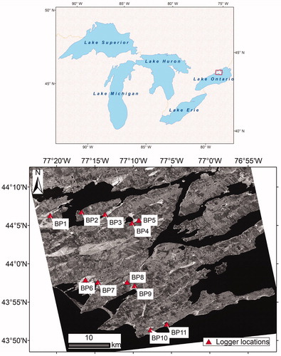
InSAR observations were used to characterize changes in scattering behavior and to infer changes in water elevation for three wetland classes, including: shallow water, marsh and swamp. Marsh is common in Bay of Quinte, characterized by an interspersion of marsh meadow and emergent aquatic vegetation, primarily cattail (Typha spp.). Cattail is normally 2–3 m tall and is capable of forming dense stands. Swamp contains 30% or more woody vegetation, including shrubs and trees, with those in the study area dominated by deciduous trees. Shallow water wetlands represent the transitional area between open water and marsh, and they can contain emergent and floating aquatic vegetation by the end of the growing season (Banks et al. 2019; Dabboor et al. 2019). Shallow water wetlands are less common than both marsh and swamp in the study area.

A total of 88 Radarsat-2 scenes were collected during 2016–2018 including FQ5W, FQ17W, U7W2 and U22W2 modes (Table 1 and Figure 1). The FQ5W and FQ17W datasets of Wide Fine Quad-Pol mode were quad-polarized (HH, HV, VH, VV) while the U22W2 and U7W2 datasets of Wide Ultra-Fine mode were single polarized (HH). A total of 20 TerraSAR-X scenes were collected in 2016 including StripFar-005 and StripFar-012 modes. The StripFar-005 and StripFar-012 datasets of Stripmap mode were dual-polarized (HH, VV). Only two ALOS-2 FBDR scenes of Stripmap Fine Beam mode acquired on May 20 and August 26, 2018 were available for this study. The FBDR datasets were dual-polarized (HH, HV) as well.

Table 1. SAR data used for the InSAR analysis.

Sensor	Mode	Polarization	resolution (range × azimuth)	Incidence angle (degrees)	Repeat cycle (days)	Number of scenes acquired
						2016	2017	2018
Radarsat-2	FQ5W	HH, HV, VH, VV	13.1 × 12.2	24	24	10	7	9
Radarsat-2	FQ17W	HH, HV, VH, VV	8.8 × 8.5	37	24	9	7	8
Radarsat-2	U7W2	HH	2.8 × 2.6	35	24	9	8	7
Radarsat-2	U22W2	HH	2.2 × 2.2	46	24	0	8	6
TerraSAR-X	StripFar-005	HH, VV	3 × 6.6	27	11	13	0	0
TerraSAR-X	StripFar-012	HH, VV	1.8 × 6.6	41.5	11	7	0	0
ALOS-2	FBDR	HH, HV	8.7 × 5.3	31.4	14	0	0	2

To aid in the identification of wetland vegetation cover and water level measurements, several field visits between April and November were completed in 2016, 2017 and 2018 for instrumentation and acquisition of 10 cm resolution UAV imagery. Since the Bay of Quinte is a relatively flat area, a digital elevation model (DEM) of 30 m spatial resolution from the Shuttle Radar Topography Mission (SRTM) was used to provide elevation information for image georeferencing and InSAR processing. Solinst pressure transducers and barometers were deployed to collect in-situ water level and barometric pressure measurements for the April-November period (all years), with two locations in marsh in 2016, seven locations in marsh in 2017, five locations in marsh, and two locations in swamp in 2018 (Table 2, Figure 1).

Table 2. Information about in-situ water level loggers.

Logger name	Measurements availability (year)	Wetland type	Water level control (Yes/No)
BP1	2016	Marsh	No
BP2	2016–2018	Marsh	No
BP3	2017–2018	Marsh	No
BP4	2018	Swamp	No
BP5	2018	Swamp	No
BP6	2017	Marsh	No
BP7	2017	Marsh	No
BP8	2017–2018	Marsh	Yes
BP9	2017	Marsh	No
BP10	2017–2018	Marsh	Yes
BP11	2018	Marsh	Yes

Methodology

Analysis of available SAR data included evaluation of backscatter, coherence, and water levels through time. First, the traditional InSAR co-registration was applied. All the InSAR images from one orbit (same sensor, polarization, and incidence angle) were co-registered and resampled to the same reference image. Multi-looking and resampling were applied to make all products of U7W2 and U22W2 at 10 m, FQ5W and FQ17W at 30 m, StripFar-005 and StripFar-012 at 10 m, and FBDR at 20 m. Selection of the final resolution for each mode was based on the resolution of the original and the need for spatial averaging to reduce the speckle effects and to estimate the coherence. To compare the backscatter from different sensor and modes, the radiometric calibration was applied to correct the antenna gain, and to normalize the reference area and range spreading loss. Then, traditional D-InSAR processing was applied to generate differential interferograms from InSAR pairs. Coherence and phase changes were then estimated from the interferograms. All InSAR processing was performed using GAMMA software.

For the backscattering and coherence analysis, statistics were generated for all dates (April–November in 2016–2018) in order to characterize the influence of sensor characteristics (e.g. polarization, frequency, resolution, incidence angle, acquisition revisit interval), vegetation condition (e.g. vegetation type and phenology), and water level. In total, 33 polygons were digitized based on visual interpretation of UAV imagery, and field visits to represent areas with marsh, shallow water, and swamp. All regions were at least 100 × 100 m in size so that they could be identified from images with different resolutions. 14 of the 33 polygons contained marsh (dominated by cattail), 11 polygons contained swamp, and eight polygons represented shallow water. For each year, the shallow water area first contained only open water, then some lily pads or cattails during the peak of the growing season.

The same sites were used to evaluate all seven datasets. Changes in backscattering coefficients and coherence over those polygons within the study period were calculated and then averaged over each wetland type. The average intensity value was also converted to decibels (dB in σ°). Both backscattering coefficients and coherence of the three wetland types in HH, HV and VV polarization from different modes were evaluated and compared. By doing this, the SAR sensitivity to detect different wetland types was investigated, and the seasonal phenological changes were characterized. The marshes and swamps with consistently high coherence values were then identified for potential water level monitoring. Shallow water area was not selected for water level monitoring due to very low coherence.

In the water level analysis using time series InSAR observations, SAR images of the same orbit were processed to produce interferometric pairs. The phase of co-registered image pairs was subtracted from each other to generate the differential interferogram. Then, the elevational changes along the radar line of sight (LOS) projection over the period between two acquisitions were produced after the removal of topographic effects. The interferograms were improved using adaptive filtering (Goldstein & Werner, 1998), and unwrapped using the Minimum Cost Flow algorithm (Costantini, 1998). Once the interferograms were correctly unwrapped, only those which maintained high coherence in wetland areas were kept for the SBAS analysis. To remove trend errors, an urban area near the town of Picton was used as a reference, assuming no significant movement during the study period. By selecting a location in the center of the study area as a reference point for InSAR analysis, atmospheric and orbital signals proportional to the distance between the reference and water level loggers was minimized due to the close distance between the reference point and observation area (Samsonov et al. 2014). The coherent observation area was identified using a coherence threshold of 0.3, after which a water level change map with respect to the reference pixel was computed to provide relevant information only to those pixels with high coherence. The regions with coherence values below the threshold were unsuitable for InSAR processing.

Using interferograms with short spatial and temporal baselines, the SBAS technique was used to maximize the temporal sampling rate of displacements calculated from the differential InSAR analysis. Cumulative changes along radar LOS from the first acquisition date was calculated from the SBAS analysis. Cumulative water level measurements corresponding to the InSAR acquisitions were also calculated from daily average water levels measured from the water loggers. A linear regression trend was built to model the relationship between the in-situ measurements and InSAR observations. R square and root mean square errors (RMSE) were calculated to determine the significance of the results. InSAR results were only validated in marsh and swamps as shallow water did not stay coherent.

Results

Characterizing wetland using backscattering and coherence

Sensitivity of backscattering to seasonal changes in the wetland

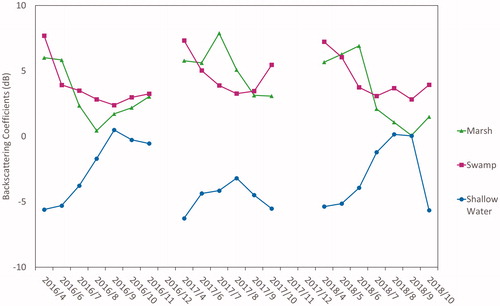
Trends of intensity changes of three wetland types during 2016-2018 were analyzed in the study area. In general, changes of HH backscatter are often indicative of double bounce scattering interactions, which can be indicative of dominant changes in wetland plant phenology. σ° for marsh, swamp and shallow water from the HH polarization in X band were similar to those in C-band. The temporal pattern of backscattering in swamp, marsh and shallow water can be illustrated using the σ° changes of the HH polarization from FQ17W (Figure 2). The σ° from swamp was the highest in April and declined as the growing season progressed when leaves were growing, and the canopies were closing. Increasing σ° of marsh during April-June corresponded to the rapid growth of cattail, while the lowest σ° values of shallow water in April were as a result of this class containing mostly open water (no live green vegetation, or little dead or senesced vegetation), resulting in predominant specular reflection. The increase in σ° values for shallow water in August and September was due to the onset of vegetation growth and emergence from the water surface. σ° values of swamp in HH polarization were higher than marsh in April-May and October-November, but lower than marsh in the growing season. This was due to a higher proportion of double-bounce to volume scattering in the early season (during leaf off), followed by predominant volume scattering following the leaf-out of the canopy.

Figure 2. Intensity changes over wetland in HH polarization from Radarsat-2 FQ17W mode.

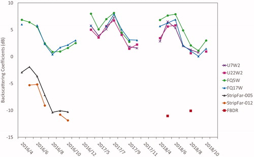
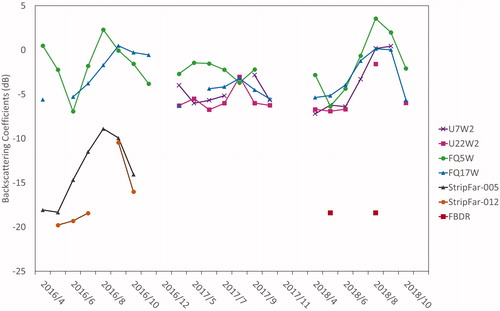
The σ° value for marsh peaked during April-June, then declined throughout the remainder of the growing season in all four modes in C-band in 2016–2018, and two modes in X-band in 2016 (Figure 3). Then, σ° values increased just after September. Notably, a secondary peak between July and August was also observed in 2017 due to historic flooding throughout the region. σ° values of marsh were also generally higher in 2017 and 2018 than 2016 due to higher water levels. Backscattering in L-band data from only two acquisition dates in 2018 was lower than that from C-band observations due to increase in size of the SAR wavelength relative to the wetland vegetation, resulting in higher penetration and decreased canopy interaction.

Figure 3. Intensity changes over marsh in HH polarization from Radarsat-2 (U7W2, U22W2, FQ5W, FQ17W), TerraSAR-X (StripFar-005, StripFar-012) and ALOS-2 (FBDR).

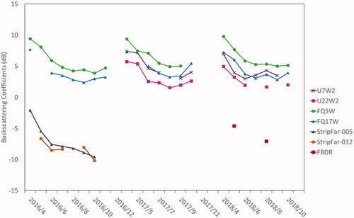
σ° values of swamp were high in April, then declined throughout the rest of the growing season in all six modes in C- and X- band in 2016–2018 (Figure 4). Similar to the trend of marsh, σ° values of swamp for the same period were generally higher in 2017 and 2018 than 2016. Backscattering of swamp in L-band data was also lower than that from C-band observations. The σ° of swamp from HH polarization in both X- and C-band during leaf off seasons were 2–6 dB higher than leaf on seasons. The lower σ° values during leaf on season was probably caused by the weaker penetration into top tree canopies which resulted in less double bounce.

Figure 4. Intensity changes over swamp in HH polarization from Radarsat-2 (U7W2, U22W2, FQ5W, FQ17W), TerraSAR-X (StripFar-005, StripFar-012) and ALOS-2 (FBDR).

σ° values for shallow water were the lowest in May and peaked in August in all six modes in C- and X-band in 2016-2018 (Figure 5). σ° showed less variation in 2017 due to the long period of high water level compared to 2016 and 2018. σ° of shallow water observed with the L band data was also lower than that from C-band observations. The high σ° values in late summer resulted from increased volume and double bounce scattering from the emergent and floating aquatic vegetation such as cattail and lily pad.

Figure 5. Intensity changes over shallow water in HH polarization from Radarsat-2 (U7W2, U22W2, FQ5W, FQ17W), TerraSAR-X (StripFar-005, StripFar-012) and ALOS-2 (FBDR).

Comparison of sensitivity of polarizations and incidence angles to the seasonal variations in wetland

Annual time series of the backscattering of marsh, swamp and shallow water from HH, HV and VV polarizations revealed spatial and temporal patterns that were aligned with seasonal changes in plant phenology and hydrological cycles. Based on the three years of C-band Radarsat-2 data in FQ5W and FQ17W modes (Table 3), values in the HH polarization were highest, followed by VV, and HV. Observations from dual-pol X-band TerraSAR-X StripFar-005 and StripFar-012 modes in 2016 also indicated that higher backscatter in HH than VV polarization. The higher HH to VV ratio also indicated higher double bounce than surface scattering which was expected in these wetland environments.

Table 3. The range of backscatter values of marsh, swamp and shallow water from the HH polarization in the study area (unit: dB).

	2016		2017		2018
	min	max	min	max	min	Max
U7W2
Marsh	NA	NA	1.6	7.3	0.8	6.5
Swamp	NA	NA	3.0	7.4	3.0	7.0
Shallow water	NA	NA	−6.0	−2.8	−7.2	0.4
U22W2
Marsh	NA	NA	1.5	6.7	0.6	5.8
Swamp	NA	NA	1.5	5.7	1.7	5.0
Shallow water	NA	NA	−6.7	−3.0	−6.9	−1.6
FQ5W
Marsh	0.9	6.9	2.8	8.1	1.1	7.9
Swamp	3.9	9.4	4.9	9.4	5.0	9.8
Shallow water	−6.9	2.3	−3.7	−1.4	−6.4	3.6
FQ17W
Marsh	0.4	6.0	3.1	7.9	0.1	6.9
Swamp	2.4	7.7	3.3	7.3	2.8	7.2
Shallow water	−5.6	0.5	−6.3	−3.2	−5.6	0.2
StripFar-005
Marsh	−10.4	−1.9	NA	NA	NA	NA
Swamp	−9.6	−2.0	NA	NA	NA	NA
Shallow water	−18.3	−8.9	NA	NA	NA	NA
StripFar-012
Marsh	−11.9	−5.2	NA	NA	NA	NA
Swamp	−10.2	−6.6	NA	NA	NA	NA
Shallow water	−19.8	−10.4	NA	NA	NA	NA
FBDR
Marsh	NA	NA	NA	NA	−11.0	−10.1
Swamp	NA	NA	NA	NA	−7.1	−4.6
Shallow water	NA	NA	NA	NA	−18.4	−18.4

Seasonal differences in the range of σ° values of wetlands varied for each polarization. Although each mode offered its own variations in σ° in response to the combination of sensor characteristics and vegetation change, there were patterns observed from the three wetland types included in this study. The pattern of σ° changes in different polarizations may be illustrated using observations of FQ17W in 2018 (Tables 4 and 5). The seasonal range of values in swamp was greater for HH polarization than VV and HV polarizations. Variations in σ° values of HV and VV polarization in swamp was small compared to that in marsh and shallow water. For example, the ranges of σ° values in a season in HV and VV were only 1.6 and 1.3 dB respectively for swamp, then became 4.2 and 7.1 dB, respectively for marsh, and reached to 9.3, 7.8 dB, respectively for shallow water. The large variation in σ° values found in shallow water may be attributed to the sensitivity of polarization to inhomogeneity of various submergent vegetation types and their growth. It was also observed that although differences in σ° values between swamp and marsh were small in HH polarization during the growing season, differences were more visible in HV and VV polarizations during July-September. The largest difference was observed from VV polarization in late August–September, reaching up to 3–5 dB in FQ17W of 2018 (Table 4).

Table 4. Backscatter changes of marsh and swamp in 2018 observed from FQ17W.

Date	HH		HV		VV
	Marsh	Swamp	Marsh	Swamp	Marsh	Swamp
2018-04-17	5.7	7.2	−5.2	−3.0	0.8	3.6
2018-05-11	6.3	6.1	−3.9	−2.6	3.6	3.4
2018-06-04	6.9	3.7	−3.4	−3.7	2.8	2.3
2018-07-22	2.1	3.1	−7.0	−3.7	−3.0	2.7
2018-08-15	1.1	3.7	−6.6	−3.2	−2.7	3.1
2018-09-08	0.1	2.8	−7.6	−4.2	−3.5	2.3
2018-10-26	1.5	3.9	−6.0	−3.4	−1.4	2.6

Table 5. The range of backscatter values of marsh, swamp and shallow water from the HH, HV and VV polarizations of Radarsat-2 FQ17W in the study area (unit: dB).

	2016		2017		2018
	Min	Max	Min	Max	Min	Max
HH
Marsh	0.4	6.0	3.1	7.9	0.1	6.9
Swamp	2.4	7.7	3.3	7.3	2.8	7.2
Shallow water	−5.6	0.5	−6.3	−3.2	−5.6	0.2
HV
Marsh	−7.0	−2.9	−7.0	−4.0	−7.6	−3.4
Swamp	−3.7	−2.3	−3.8	−2.2	−4.2	−2.6
Shallow water	−16.2	−8.5	−16.5	−11.1	−16.2	−6.9
VV
Marsh	−2.0	2.7	−1.8	5.1	−3.5	3.6
Swamp	2.3	4.0	2.5	4.1	2.3	3.6
Shallow water	−5.7	0.1	−6.7	−1.7	−7.4	0.5

The variation of σ° in the wetlands was also closely related to the incidence angle. In general, backscattering from steeper incidence angles was stronger than the shallower incidence angles. Results showed that σ° was inversely related to the incidence angles (Table 3). For example, both U7W2 and U22W2 had similar spatial resolution (2.8 vs. 2.2 m) but different incidence angles (35 vs. 46 degrees). The σ° of shallow water in HH polarization ranged −7.2 to 0.4 dB in U7W2 images in 2018 compared to −6.9 to 1.6 dB in U22W2 images. Similar observations were found in the swamp and shallow water. Comparison of modes FQ5W with FQ17W, StripFar-005 with StripFar-012 which had similar resolution but different incidence angles also showed the differences in σ°. Among these modes, the FQ5W had the highest σ° because the surface was imaged at a steeper incidence angle, resulting in more direct backscatter returns in the direction of the sensor.

Results from coherence analysis over wetlands

Results from the coherence analyses showed that the cattail dominated marsh had the highest values for all four modes of C-band and two modes of X-band SAR data, followed by swamp, and shallow water had the lowest coherence (Table 6). Coherence in C-band was higher than in X-band for the same wetland type, given the same acquisition interval (22 − 24 days). The coherence values for marsh and swamp from C- and X-band were highest in April-May and October-November. During the growing season, the coherence of swamp was very low (below 0.4) because the leaf out of the canopy and low water level reduced double bounce. The difference in coherence between swamp and shallow water was greater with the X than the C-band data.

Table 6. Average coherence from April to November for wetlands in the study area (ALOS2 has only one pair).

Mode	Polarization	Year	Marsh	Swamp	Shallow water
U7W2	HH	2016–2018	0.64	0.44	0.35
U22W2	HH	2017–2018	0.65	0.47	0.33
FQ5W	HH	2016–2018	0.70	0.51	0.34
FQ5W	HV	2016–2018	0.55	0.36	0.30
FQ5W	VV	2016–2018	0.61	0.43	0.33
FQ17W	HH	2016–2018	0.65	0.40	0.38
FQ17W	HV	2016–2018	0.48	0.29	0.31
FQ17W	VV	2016–2018	0.52	0.35	0.30
StripFar-005	HH	2016	0.74	0.35	0.32
StripFar-005	VV	2016	0.60	0.33	0.31
StripFar-012	HH	2016	0.58	0.26	0.30
StripFar-012	VV	2016	0.44	0.27	0.28
FBDR	HH	2018	0.43	0.68	0.36
FBDR	HV	2018	0.46	0.57	0.29

With three years of Radarsat-2 observations, similar temporal trends were observed within wetlands on a seasonal basis, however both the timing of change, and magnitude of coherence values differed interannually. This can be attributed to changes in environmental conditions, such as water level, vegetation composition, height, and density. For example, during high water levels in 2017, the coherence from swamp was the same or greater than marsh at times, which was not generally the case when water levels were lower. Figure 6 shows that with the HH polarization of FQ17W, coherence from swamp was similar to marsh in April-June, but higher than marsh in August of that year (Figure 6). For marsh, coherence values were generally highest early in the growing season. During this time, the marsh is made up of dead, senescent vegetation. These mostly physically stable targets could have resulted in highly consistent backscatter through time, though notably they have a random size/orientation and the dielectric properties, which could have changed due to changes in moisture content. While the growing season progressed, green healthy vegetation increased in size and density. As most of the vegetation was cattails, we expect that the observed decrease in coherence was as a result of both rapid changes in size/orientation of targets (i.e. mostly cattails). Cattails were observed to be highly mobile as a result of the effects of wind (sometimes swaying more than a meter) and in cases where the vegetation mat was not grounded to the lake-bed, mats were observed to be floating in some cases, thus resulting in a change in their horizontal position and vertical position due to changes in water level. This was exacerbated by the effects of high winds and storm surges on the lake. A return to high coherence levels at the end of the growing season signaled the return to dominance of senescent, immobile vegetation. This was for 2016 and 2018, for 2017 patterns were clearly different, though this was likely because of high water levels and storm surges pushing vegetation around etc. For swamp this rapid decline in coherence was much earlier and more dramatic since the leaf-out of the canopy (at the end of May), resulted in an immediate and dramatic decrease in the transmissivity of the canopy, leading to predominant volume scattering at the top of the canopy and a loss of double bounce which happens at the bottom of trunks.

Figure 6. Coherence change in wetland from FQ17W HH polarization.

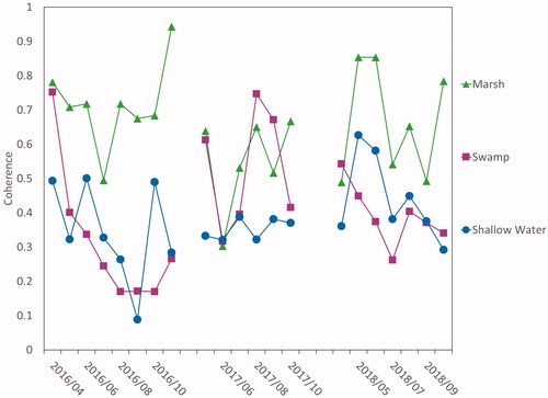
Results also demonstrated that both polarization and temporal baseline influenced the coherence in wetlands. The coherence was highest in HH, followed by VV, and was always lowest in HV. For example, average coherence values from FQ17W mode for marsh, swamp, and shallow water were 0.65, 0.4 and 0.38 from the HH polarization, and 0.48, 0.29, and 0.3 from HV polarization, 0.51, 0.35 and 0.3 from the VV polarization (Table 6).

To evaluate the influence of temporal baseline on coherence, interferograms of Radarsat-2 with 24-day and 48-day interval, and interferograms of TerraSAR-X with 11-day, 22-day, 33-day, and 44-day were generated and compared. Results showed that coherence values were inversely related to the length of the acquisition interval. The coherence of the C-band data, with a nominal 24-day acquisition interval, was, at times, significantly higher than a 48-day acquisition interval. For example, during June-July, the coherence values for marsh, swamp, and shallow water from the HH polarization of the FQ17W data in 2018 were 0.64, 0.54, and 0.54 respectively, for a 24-day acquisition interval, but dropped to 0.34, 0.28, and 0.25, respectively with a 48-day interval.

Similarly, the coherence of the X-band data during an 11-day acquisition interval was significantly higher than 22-day, 33-day, and 44-day. For example, the coherence for marsh from the HH polarization of the StripFar-005 images was 0.87, 0.74, 0.51, and 0.32 for the 11-day, 22-day, 33-day, and 44-day intervals respectively during June-July. The coherence in the swamp and shallow water from X-band was low (<0.35) with an 11-day cycle and did not change greatly with an increase of the temporal baseline. Average coherence from StripFar-005 was higher than StripFar-012 due to the fact that six pairs of StripFar-005 images were acquired with an 11-day cycle compared to none from StripFar-012. Unlike the backscattering, difference of incidence angles did not cause noticeable variation in coherence.

The lack of time series observation from L-band data prevented the comparison with X- and C-band directly in the study. The seasonal coherence variation of wetland from L-band was not available either. However, different from C- and X-band data, coherence for the wetland from both HH and HV polarizations in the only available pair of L-band was maintained over a very long period. Swamp had the highest coherence values, followed by marsh, and shallow water had the lowest coherence. For example, the coherence for swamp, marsh, and shallow water with the pair of HH polarized data acquired with even a 98-day interval was 0.68, 0.43, and 0.36, respectively.

Results from water level analysis

The clear fringe patterns observed within wetlands demonstrated potential to use InSAR for monitoring changes in water level through space and time. Results from these analyses showed that SAR data with finer spatial resolutions produced clearer fringe patterns. For example, during the May–June season, clearer patterns in the marsh could be observed from the interferograms generated from finer resolution modes, such as U7W2, U22W2, StripFar-005, and StripFar-012, compared to coarser resolution modes FQ5W and FQ17W (Figure 7B–H). However, the fringe patterns became much less obvious after June due to changing environmental conditions (a decrease in water level, an increase of cattail and leaf density in marsh and forest canopy in swamp), which resulted in a decrease in double bounce and lower coherence.

Figure 7. Interferograms of marsh generated using data of HH polarization from different modes using pairs acquired in May-June. (A) Google Earth image; (B) U7W2: 2018/05/29_2018/06/22; (C) U22W2: 2018/05/21_2018/06/14; (D) FQ5W: 2018/05/15_2018/06/08; (E) FQ17W: 2018/05/11_2018/06/04; (F) StripFar-005: 2016/05/18_2016/06/09; (G) StripFar-012: 2016/05/23_2016/06/14; (H) StripFar-005: 2016/06/09_2016/06/20.

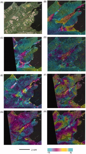
Clear changes were also observed from X-band StripFar-005 and StripFar-012 modes due to its increased sensitivity to changes in target characteristics (e.g. size, orientation, horizontal/vertical position) because of its shorter wavelength (Figure 7F–H). With an 11-day acquisition interval, more detailed information on changes in hydrology were revealed by the X-band data (Figure 7H). Interferograms from swamp from the C- and X- band data during the leaf off season also showed clearer patterns than that during the leaf on season because of the higher coherence maintained during the former.

Field measurements at two locations in 2016, and seven locations in 2017 and 2018 were used to validate the InSAR results in the Bay of Quinte. A correlation analysis produced mixed results in different locations depending on SAR mode and season (Tables 7 and 8). Although positive correlations between field measurements and InSAR observations from different modes were shown in two locations in marsh in 2016, mixed results (both positive and negative correlations) were found in all locations in 2017 and 2018. For example, a strong positive correlation between field measurements and InSAR observations was calculated in all three modes including U7W2 (Figure 8A), FQ5W and FQ17W in 2018 from both the marsh sites of BP3 and BP10 and the swamp site of BP4 (Table 8).

Figure 8. Comparison of cumulative water level changes from logger measurements with InSAR measurements from Radarsat-2 with the HH polarization. (A) U7W2 results for marsh site BP1 in 2016, (B) U7W2 results for swamp site BP4 in 2018, (C–D) FQ5W results for marsh site BP3 in 2017 and 2018.

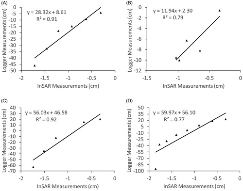
Table 7. Comparison of InSAR results and field water level measurement in Bay of Quinte in 2016 (HH polarization, RS2: Radarsat-2, TX: TerraSAR-X).

	RS2-U7W2		RS2-FQ5W		TX-StripFar-005
Location	R	RMSE	R	RMSE	R	RMSE
BP1	0.95	24.2	0.94	32.8	0.98	28.2
BP2	0.91	25.1	0.23	34.7	0.94	29.2

Table 8. Comparison of InSAR results and field water level measurement in Bay of Quinte in 2017–2018 (HH polarization, RS2: Radarsat-2).

	RS2-U7W2				RS2-U22W2		RS2-FQ5W				RS2-FQ17W
	2017		2018		2017		2017		2018		2017		2018
Location	R	RMSE	R	RMSE	R	RMSE	R	RMSE	R	RMSE	R	RMSE	R	RMSE
BP2	0.93	62.3	−0.93	37.1	0.95	48.8	0.96	31.9	0.93	30.7	−0.98	64	−0.99	24.9
BP3	0.97	62	0.99	31.2	0.97	48.5	0.96	33.6	0.87	38.4	−0.54	61.6	0.97	23
BP4	NA	NA	0.87	13.7	NA	NA	NA	NA	0.86	31	NA	NA	0.90	17.1
BP5	NA	NA	0.89	6.9	NA	NA	NA	NA	0.01	21.7	NA	NA	−0.08	33.4
BP6	−0.74	63	NA	NA	0.99	40.6	0.96	31.1	NA	NA	−0.96	63.9	NA	NA
BP7	0.98	57.2	NA	NA	0.99	42.2	0.96	30.7	NA	NA	−0.96	64.2	NA	NA
BP8	−0.70	11.9	−0.90	2.6	0.85	17.5	0.92	16.7	0.77	4	0.00	12.5	−0.73	10.6
BP9	0.98	48.2	NA	NA	0.98	38.7	0.97	28.5	NA	NA	−0.94	55.2	NA	NA
BP10	−0.94	32.5	0.95	31.4	−0.39	34.3	0.91	29	0.91	51.6	−0.52	27.9	0.99	48.9
BP11	NA	NA	−0.97	26.3	NA	NA	NA	NA	−0.94	30.6	NA	NA	0.95	35.8

However, results from three modes were contradictory in the other four sites. In particular, low correlation was found in the swamp site of BP5 from FQ5W and FQ17W modes, despite a strong positive correlation with U7W2 in 2018 (Figure 8B). These results complicated our understanding of the effect of changing environmental conditions on the InSAR results. Therefore, it was not possible to conclude the effect of incidence angle and resolution on InSAR measurements. If the performance of SAR data modes was evaluated only based on the positive correlation and smaller RMSE values between InSAR and in-situ measurements, results indicated that the finer resolution mode U7W2 performed better than other modes in swamp, and FQ5W performed better in marsh (Figure 8).

The maximum RMSE values for results in 2016, 2017, and 2018 were 35, 64, and 52 respectively. These large RMSE values indicated low potential for the linear regression model fitted to accurately predict water level from InSAR derived deformation values. We attribute this low measure of fit to observed temporally and spatially dynamic water levels, for which daily values varied by up to 22 cm. Each year also showed its own variations due to the influence from combined conditions including precipitation, temperature, barometric pressure and wind. Based on available data for the entire study period, water level fluctuated the most in April 2018, though unfortunately, water level information was not available for April 2016 and April 2017 (Figure 9).

Figure 9. Daily water level change in 2016–2018 in Robinson Cove (BP2) (related to SAR acquisitions, water level from May 12, 2016 was the reference for 2016, May 2, 2017 was the reference for 2017 and April 5, 2018 was the reference for 2018).

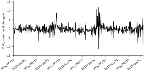
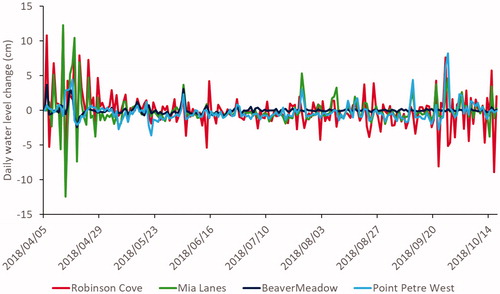
The fluctuations of lake water can significantly influence the water level in the wetlands that are hydrologically linked to the lake, whereas runoff and precipitation affect those inland. It was observed that fluctuations in wetlands connected to the channels of Lake Ontario were greater than inland wetlands. In the study area, water level change in marsh with natural hydrological connections has more fluctuations than those inland wetlands. For example, the daily water level in the marsh (BP2) in the natural water conditions (e.g. water level not controlled) had more fluctuations than the swamp (BP4) which was connected to an inland lake. However, both varied greatly in April, and late September to October 2018. The largest variation ranged from 12 to −12 cm during April 13 and April 14 in both the marsh and swamp.

Water level in the controlled marsh area did not exhibit natural water level fluctuations. Unlike those wetlands linked to the lake, for example, the largest variation in BP8 and BP10 ranged from only 4.4 to −2.4 cm on April 16 and April 19 (Figure 10).

Figure 10. The daily water level change in Bay of Quinte in 2018 (BP2: a marsh connected to the channel of Lake Ontario (red), BP 4: a swamp connected to an inland lake (green), BP8 (dark blue) and BP10: marshes with controlled water level management (light blue)).

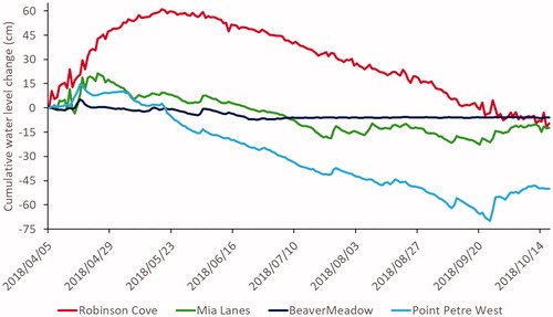
Differences in daily water levels also affected cumulative water levels. For example, the cumulative water level at location BP2, a marsh that was connected to the channel of Lake Ontario, maintained an increasing trend until reaching a maximum of 61 cm on May 19, then values decreased though the cumulative water level remained positive until September 19 (Figure 11). The increasing trend of cumulative water level at BP4, a swamp that was connected to an inland lake, only lasted until April 24, when a maximum difference of 21 cm was recorded. Here, the cumulative water level remained positive until June 21. At BP8, a marsh for which water levels were controlled, cumulative water levels reached a maximum of 5.3 cm on April 17, then remained close to zero throughout the rest of the season. At BP10, another marsh with a controlled water level, the cumulative water level became negative starting from May 20, and remained negative until the end of study period. However, a minimum cumulative water level of −70 cm was observed on September 24 at this location. The daily variation and cumulative change of water level in wetlands may not be observed by InSAR observations completely due to the small variation of InSAR phase changes.

Figure 11. Cumulative water level change in Bay of Quinte in 2018 (BP2: a marsh connected to the channel of Lake Ontario (red), BP 4: a swamp connected to an inland lake (green), BP8 (dark blue) and BP10: marshes with controlled water level management (light blue)).

The combined effects of high fluctuations in water levels over short time periods and the relatively long intervals between SAR observations may have resulted in the variable correlation and large RMSE between water level and InSAR measurements in the study area. For example, the cumulative water level change at BP3 during the FQ5W acquisition period of April 21–October 30, 2018 was −95 cm, though the cumulative displacement from InSAR observations was only −1.9 cm (Figure 8D). Large RMSE values were calculated in the marsh with natural hydrological conditions such as at locations BP1, BP2, and BP3, and also the marsh with controlled water conditions but discharged into the Lake Ontario directly such as locations at BP10 and BP11.

Most interferograms in Bay of Quinte had only half a fringe compared to 1–2 fringes in Long Point (Chen et al. 2020). Fewer interferogram fringes meant that less changes in elevation spatially were observed from InSAR which resulted in higher RMSE values between InSAR and in-situ field measurements in the marsh of Bay of Quinte comparing to the results in Long Point. Results from this, and a previous study in Long Point (Chen et al. 2020) may confirm that C-band data have fringe saturation (e.g. the increase of fringe frequency is limited despite the large variation of the movement of the object) in areas like Bay of Quinte and Long Point, where there is high-water level change (both daily water level and accumulated water level >10 cm). Theoretically, at least four fringe cycles to be observed from an interferogram in order to monitor a water level change >10 cm considering each fringe cycle in C-band only represents 2.8 cm (half of wavelength) change. In real environment when large phase changes distributed across limited coherent wetland areas, accurate phase unwrapping is challenging. For example, although the marsh in Bay of Quinte exhibited high coherence and correlations between InSAR measurements and water level changes, the RMSE was high (3–64 cm). High RMSE values indicate high levels of uncertainty associated with the relationship between InSAR and field measurements. The low coherence in swamp also resulted in weak correlation between field measurements and InSAR observations in FQ5W and FQ17W modes in one of the swamp areas. As such, frequent observations from L-band data is needed to improve the coherence in swamp and InSAR measurements.

The effects of incidence angle on the InSAR measurements were evaluated using the observations which produced a positive correlation only, as it was assumed that at these sites at least the direction of change could be predicted. Comparison between high resolution mode U7W2 and U22W2 data indicated that InSAR measurements from the latter, in 2017, which had a shallower incidence angle, offered a smaller RMSE value. Similarly, the InSAR measurements in 2018 from the FQ17W data, which also had shallower incidence angle, offered smaller RMSE values than the FQ5W data. The comparison of results between U7W2 with FQ5W in 2016, U22W2 with FQ17W in 2017, U7W2 with FQ17W in 2018, also indicated that data with finer resolution produced smaller RMSE values. As the water level in 2017 was exceptionally higher than 2016 and 2018, and given the fact that results from FQ5W in 2017 were the best among all modes in terms of RMSE values, we speculate that the steeper incidence angle could have resulted in further penetration through the canopy, resulting in higher probability of scattering from the water surface though this depends on the vegetation size/wavelength ratio. The effect of coarse resolution and incidence angle on InSAR measurements at high water level needs to be further studied in future.

Based on results from the coherence analysis, pattern of interferograms, and water level analysis, it was found that generally, InSAR data with finer resolution, and HH polarization were preferred for monitoring water level change within wetlands. In particular, C-band was suitable for monitoring marsh and L-band for monitoring swamp. Finer resolution SAR data represented change within small wetlands more accurately and were able to generate interferograms with clearer fringe patterns, thus provided more detailed hydrological changes in the study area. Temporal resolution was found to be very important for maintaining coherence and monitoring these wetlands. For example, given an 11-day interval, TerraSAR-X data maintained good coherence and produced high correlation with field measurements in the marsh. In contrast, no clear fringes were seen over the wetland from interferograms generated from L-band data with HH and HV polarization, though coherence was still high in the wetland in the L-band pair over 98 days.

Discussion

Spatio-temporal changes in backscatter and coherence from various SAR data over three years were interpreted as the response to temporal and spatial patterns of water level change, as well as plant phenology. Such information is important for exploring the potential of using InSAR to monitor water level changes in wetlands along the coast of the Great Lakes. A recent study using C-band Radarsat-2 HH polarization and Sentinel-1 VV polarization (Chen et al. 2020) has indicated that high coherence was observed from marsh with mixed cattail and Phragmites in the Great Lakes. In this study, InSAR analysis was expanded to study both marsh and swamp in the Great Lakes using various polarizations X-, C- and L-band.

Observations indicated that backscattering from swamps was higher during the leaf off season than during leaf on season, and the seasonal difference was greater for HH polarization than VV and HV polarizations. Similar seasonal differences were found with C-band Radarsat-1 HH and ERS1/2 VV data in a Louisiana swamp (Lu and Kwoun 2008). The high σ° and coherence in swamp during the leaf-off season was caused by double-bounce scattering, which has also been reported in flooded forests elsewhere (Wdowinski et al. 2008; Brisco et al. 2015; Brisco et al. 2017). The unique characteristics of phenological change within swamps have been exploited to distinguish it from marsh between April and May (Banks et al. 2019), and could be expanded to October-November because swamp had higher σ° values than marsh in all polarizations during both time periods. However, the classification of marsh and swamp can be a challenge during the growing season (Banks et al. 2019), especially with just the HH polarization, due to increasing σ° values of marsh (i.e. within a similar range as those observed for swamp). Backscatter analysis indicated that the separability of these two classes could be improved by combining HH polarization with HV or VV polarizations because the difference between σ° values of swamp and marsh was more visible in HV and VV polarizations during July-September.

In a previous study in Florida’s wetlands using TerraSAR-X (Hong, Wdowinski, and Kim 2010), all polarizations (HH, HV, and VV) exhibited similar interferogram patterns although HH polarization performed the best. In this study, despite the difference in backscatter intensity and coherence, only HH and VV exhibited similar interferogram patterns, nevertheless patterns from VV were less clear than HH. No clear interferogram patterns were observed from HV C-band data. We speculate that the difference of interferogram quality from HH, VV and HV was related to the difference in coherence values. As coherence in HH was generally 17–20% higher than VV in both marsh and swamp, and up to 25% higher than HV, the latter was not useful for generating interferograms with clear patterns. It was difficult to determine if different spatial deformation information could be revealed from different polarization due to limited changes in fringe rate in the study.

Our observations using HH and VV polarizations from both Radarsat-2 and TerraSAR-X confirmed that high coherence could be maintained over cattail marsh which supports findings using C-band data reported in Chen et al. (2020). Results showed that X-band SAR did not generate high coherence over swamp compared to C- and L-band data. This indicates that the shorter wavelength X-band signal interacted mostly with the upper sections of vegetation such as tree canopies and branches, which was different from the observation in Florida’s Everglades wetlands where X-band demonstrated high coherence over the mangrove wetland (Hong, Wdowinski, and Kim 2010). Coherence from swamp in C-band also varied by season which made the time series InSAR observation unstable and inaccurate. Despite the long acquisition period, coherence from our only available L-band pair was still high enough for applying InSAR techniques to both marsh and swamp, however, fringe patterns were not clear, thus posed a challenge to link to the variation of water level. Further investigation of InSAR monitoring of water level in the Great Lakes using time series L-band data is needed to make a conclusion.

Results from comparison of the coherence from HH polarization indicated that the smaller (steep) incidence angle produced slightly higher coherence values than shallow incidence angles. For example, FQ5W has the coherence values of 0.7 and 0.5 from marsh and swamp which were the highest among C-band Radarsat-2 modes, StripFar-005 from X-band achieved the coherence values of 0.74 and 0.35 from marsh and swamp which were higher than StripFar-012. However, comparison of the R and RMSE values from the regression of InSAR and water level measurements indicated that shallow incidence angles performed better with higher R and smaller RMSE values. From our understanding, SAR can penetrate the marsh vegetation, and cause double bounce between water surface and vertical structures which is critical for InSAR analysis. However, we didn’t have enough dataset for validating if incidence angles had influence on double bounce scattering. The effects of incidence angles were not fully assessed and further investigation is needed.

In the analysis, we did not separate swamps with dead trees from swamps with living trees, though because seasonal changes in coherence were observed as a result of the leaf-out of the canopy (i.e. with higher values observed between April-May and lower values between June-October), we anticipate that coherence values also vary as a result of various stand characteristics, including the presence of both living and dead trees. Therefore, further analysis of coherence and InSAR performance over various swamps is needed to fully understand and utilize such differences, which are indicative of both different habitat types and or changing vegetation conditions.

Floating marsh vegetation and wind condition may affect InSAR observations. It is believed that cattail may grow on a floating mat which can rise and fall with water level. We suspect such floating condition may have also affected the path length of double bounce between water surface and vertical structure of cattail and consequently the InSAR measurements. Wind speed and direction may also have contributed to the movement of cattail marsh resulting in uncertainties in coherence estimation and InSAR measurements. These influences maybe studied in future.

Based on the results in Lake Ontario in this study, and in Lake Erie (Chen et al. 2020), high coherence in marsh could be exploited for InSAR monitoring of wetland. However, great water level fluctuations posed a major challenge for InSAR monitoring of water level changes. Loggers located at different locations showed variation of water level changes in the study area. This spatial variation over a small area was also reported in the Long Point marsh in the Great Lakes (Chen et al. 2020). However, such variation of water level is certainly not represented by the only available water gauge station about 50 km from the study area. From this perspective, InSAR monitoring has an advantage for spatial coverage. However, InSAR observations at each location assumed constant change rate during the acquisition period which was not true given the dynamic water level changes in the Great Lakes. Although InSAR correctly predict the trend of water level changes in some locations, large RMSE indicated underestimation of water level changes. The large RMSE values observed from this study was mainly caused by three reasons. First, temporal patterns of water level changes were not fully represented by SAR observations. Large water level fluctuation over short period was not captured by sparse InSAR observations over long acquisition intervals (24 days for Radarsat-2 and 11 days for TerraSAR-X). For example, the maximum daily water level variation in the study area was −12 to 12 cm during 2018, resulting in a cumulative water level change of up to 70 cm. Cumulative information from the limited number of interferograms was not sufficient to represent the range of water level changes in the lakes even using SBAS for the time series analysis.

Second, spatial patterns of water level changes were not detected from phase changes. Low fringe density (less than two fringes) was only detected over a local wetland area that was coherent. Marshes in Bay of Quinte were small, so the coherent areas were limited as well. Phases representing water level changes could only be extracted from those coherent areas with limited fringes. We suspected that the phase changes only represented the changes of those local water surface topography. Therefore, correct phase unwrapping was difficult.

Third, the quality of interferogram was affected by seasonal variations of phenology and water level. Coherence loss in June–August and low water level season hindered the fringe generation and valid InSAR observations. Certainly, long acquisition intervals also contributed to the loss of coherence over large wetland areas, which caused difficulty in establishing quality interferograms to reflect the spatial water level changes and variation of measurements using time series InSAR.

Given large spatio-temporal changes in water level in the Great Lakes, to accurately predict water level, frequent InSAR observations are needed to improve the coherence over a large wetland area, and to increase the sampling rate of measurements for time series analysis. InSAR with shorter temporal acquisition intervals may be a viable solution for monitoring such a dynamic environment. For accurate measurement of water level changes, the frequency of InSAR acquisitions should be increased to match the water level fluctuations. For example, the Radarsat Constellation Mission (RCM) data, which has three satellites in the orbit with a four day repeat cycle, may provide more accurate measurements. InSAR potential for water level monitoring will be enhanced when frequent SAR data is available.

Conclusions

InSAR observations over the Bay of Quinte, Ontario, Canada during the years 2016–2018 from Radarsat-2, 2016 from TerraSAR-X, and 2018 from ALOS-2 satellites indicate that backscatter and coherence were sensitive to sensor characteristics (frequency, polarization, incidence angle, acquisition interval), changes in water level, and phenology. Time series InSAR measurements and in-situ water levels were compared to investigate the suitability of SAR for monitoring wetlands in the Great Lakes with dynamic water level changes. It was found that InSAR phase changes responded to the water level changes. This confirmed that X-, C-, and L-band have potential for monitoring wetland water level changes along the coast of the Great Lakes.

In terms of the coherence and interferogram quality, this study found that finer resolution suited the wetland study needs in comparison to coarser resolution and steeper incidence angles. C-band worked better than X-band in marsh, and L-band may be preferred in swamp. Time series X- and C-band data over marsh showed that HH polarization had the highest backscattering and coherence, followed by VV, and HV polarization had the lowest. However, results showed that the correlation between InSAR measurements and field water level changes varied from −1 to 1 depending on the site, type of wetland vegetation, and incidence angle. Although some sensor modes provided a good correlation (0.77–1) and predicted the trend of water level changes at a few locations, the large RMSE values between 4 and 64 cm indicated that InSAR observations of water level changes were generally underestimated. Very limited changes in InSAR fringe frequency in this study also suggested that sparse InSAR observations did not respond to dynamic spatio-temporal changes well, and the C-band and X-band interferograms may be saturated in cases of high-water level changes such as the Great Lakes. Frequent data acquisition is suggested to improve InSAR applications because higher coherence can be maintained within a shorter time period, making it possible to detect dynamic water level changes. More research is needed on the application of InSAR with RCM data once it becomes available.

Acknowledgments

We thank the Ontario Ministry of Natural Resources and Forestry for sharing the UAV data and access to Bay of Quinte for field work. Thanks to the private owners for providing access, support for in-situ instrument installation for field work. The authors thank Sergey Samsonov for providing the SBAS code. We also thank Taylor Harmer, Tom Giles, Matt Giles and Andrew Kelly from our department for their support in the field for instrument installation, data collection, and UAV data acquisition. RADARSAT-2 Data and Products © Maxar Technologies Ltd. (2018) – All Rights Reserved. RADARSAT is an official mark of the Canadian Space Agency.

Additional information

Funding

This project was funded by the Canadian Space Agency (CSA) under the project “Ecosystem Assessment and Monitoring” (RCM Data Utilization & Application Plan (DUAP) IMOU number - 14SURCM007). Radarsat-2 imagery was provided by CSA.

References

- Alsdorf, D.E., Smith, L.C.M., and Melack, J. 2001. “Amazon floodplain water level changes measured with interferometric SIR-C radar.” IEEE Transactions on Geoscience and Remote Sensing, Vol. 39(No. 2): pp. 423–431.
- Banks, S., White, L., Behnamian, A., Chen, Z., Montpetit, B., Brisco, B., Pasher, J., and Duffe, J. 2019. “Wetland Classification with Multi-Angle/Temporal SAR Using Random Forests.” Remote Sensing, Vol. 11(No. 6): pp. 670.
- Brisco, B., Ahern, F., Murnaghan, K., White, L., Canisus, F., and Lancaster, P. 2017. “Seasonal Change in Wetland Coherence as an Aid to Wetland Monitoring.” Remote Sensing, Vol. 9(No. 2):pp. 158.
- Brisco, B., Murnaghan, K., Wdowinski, S., and Hong, S.H. 2015. “Evaluation of RADARSAT-2 Acquisition Modes for Wetland Monitoring Applications.” Canadian Journal of Remote Sensing, Vol. 41(No. 5): pp. 431–439.
- Chen, Z., White, L., Banks, S., Behnamian, A., Montpetit, B., Pasher, J., Duffe, J., and Bernard, D. 2020. “Characterizing marsh wetlands in the Great Lakes Basin with C-band InSAR observations.” Remote Sensing of Environment, Vol. 242: pp. 111750.
- Costantini, M. 1998. “A novel phase unwrapping method based on network programming.” IEEE Transactions on Geoscience and Remote Sensing, Vol. 36(No. 3): pp. 813–821.
- Dabboor, M., Banks, S., White, L., Behnamian, A., Chen, Z., Montpetit, B., Brisco, B., Pasher, P., and Duffe, J. 2019. “Comparison of compact and fully polarimetric SAR for multi-temporal wetland monitoring.” IEEE Journal of Selected Topics in Applied Earth Observations and Remote Sensing, Vol. 12(No. 5): pp. 1417–1430.
- EC. 2018. Canadian Climate Normals 1981:2010. Gatineau, QC, Canada: Environment and Climate Change Canada.
- EC. 2019. Canadian Climate Normals 1981–2010 Station Data. Environment Canada. https://climate.weather.gc.ca/climate_normals/index_e.html
- Goldstein, R.M., and Werner, C.L. 1998. “Radar interferogram filtering for geophysical applications.” Geophysical Research Letters, Vol. 25(No. 21): pp. 4035–4038.
- Gownaris, N.J., Rountos, K.J., Kaufman, L., Kolding, J., Lwiza, K.M.M., and Pikitch, E.K. 2018. “Water level fluctuations and the ecosystem functioning of lakes.” Journal of Great Lakes Research, Vol. 44(No. 6): pp. 1154–1163.
- Hong, S.H., Wdowinski, S., and Kim, S.W. 2010. “Evaluation of TerraSAR-X Observations for Wetland InSAR Application.” IEEE Transactions on Geoscience and Remote Sensing, Vol. 48(No. 2): pp. 864–873.
- Hong, S.H., Wdowinski, S., Kim, S.W., and Won, J.S. 2010b. “Multi-temporal monitoring of wetland water levels in the Florida Everglades using interferometric synthetic aperture radar (InSAR).” Remote Sensing of Environment, Vol. 114(No. 11): pp. 2436–2447.
- Kim, S., Wdowinski, S., Amelung, F., Dixon, T.H., and Won, J. 2013. “Interferometric coherence analysis of the everglades wetlands, South Florida.” IEEE Transactions on Geoscience and Remote Sensing, Vol. 51(No. 12): pp. 5210–5224.
- Lu, Z., and Kwoun, O. 2008. “Radarsat-1 and ERS InSAR analysis over southeastern coastal Louisiana: Implications for mapping shallow water-level changes beneath swamp forests.” IEEE Transactions on Geoscience and Remote Sensing, Vol. 46(No. 8): pp. 2167–2184.
- Lu, Z., Crane, M., Kwoun, O.-I., Wells, C., Swarzenski, C., and Rykhus, R. 2005. “C-band radar observes water level change in swamp forests.” Eos, Transactions American Geophysical Union, Vol. 86(No. 14): pp. 141–144.
- Mohammadimanesh, F., Salehi, B., Mahdianpari, M., and Motagh, M. 2017. “X-band interferometric SAR observations for wetland water level monitoring in newfoundland and Labrador”. In 2017 IEEE International Geoscience and Remote Sensing Symposium (IGARSS), Fort Worth, TX, pp. 3159–3162.
- OMNDM. 2012. Surficial Geology of Southern Ontario. Greater Sudbury, ON, Canada: Ontario Ministry of Energy, Northern Development and Mines.
- Samsonov, S.V., González, P.J., Tiampo, K.F., and d'Oreye, N. 2014. “Modeling of fast ground subsidence observed in southern Saskatchewan (Canada) during 2008–2011.” Natural Hazards and Earth System Sciences, Vol. 14(No. 2): pp. 247–257.
- Wang, Y., and Yésou, H. 2018. “Remote Sensing Of Floodpath Lakes And Wetlands: A challenging frontier in the monitoring of changing environments.” Remote Sensing, Vol. 10(No. 12): pp. 1955.
- Wdowinski, S., Amelung, F., Miralles-Wilhelm, F., Dixon, T.H., and Carande, R. 2004. “Space-based measurements of sheet-flow characteristics in the Everglades wetland, Florida.” Geophysical Research Letters, Vol. 31(No. 15): art. L15503.
- Wdowinski, S., Kim, S.W., Amelung, F., Dixon, T.H., Miralles-Wilhelm, F., and Sonenshein, R. 2008. “Space-based detection of wetlands' surface water level changes from L-band SAR interferometry.” Remote Sensing of Environment, Vol. 112(No. 3): pp. 681–696.
- Young, M., Patterson, N., and Dunn, L. 2002. Great Lakes Coastal Wetlands – Science and Conservation. Environment Canada. http://publications.gc.ca/collections/Collection/En40-222-11-2002E.pdf.
- Yuan, T., Lee, H., Jung, H.C., Aierken, A., Beighley, E., Alsdorf, D.E., Tshimanga, R.M., and Kim, D. 2017. “Absolute water storages in the Congo River floodplains from integration of InSAR and satellite radar altimetry.” Remote Sensing of Environment, Vol. 201: pp. 57–72.
- Zhang, B., Wdowinski, S., Oliver-Cabrera, T., Koirala, R., Jo, M.J., and Osmanoglu, B. 2018. “Mapping the extent and magnitude of severe flooding induced by hurricane Irma with multi-temporal Sentinel-1 SAR and InSAR observations.” ISPRS – International Archives of the Photogrammetry, Remote Sensing and Spatial Information Sciences, Vol. XLII-3(No. 3): pp. 2237–2244.