Fusing Landsat and SAR Data for Mapping Tropical Deforestation through Machine Learning Classification and the PVts-β Non-Seasonal Detection Approach

Abstract

This article focuses on mapping tropical deforestation using time series and machine learning algorithms. Before detecting changes in the time series, we reduced seasonality using Photosynthetic Vegetation (PV) index fractions obtained from Landsat images. Single and multi-temporal filters were used to reduce speckle noise from Synthetic Aperture Radar (SAR) images (i.e., ALOS PALSAR and Sentinel-1B) before fusing them with optical images through Principal Component Analysis (PCA). We detected only one change in the two PV series using a non-seasonal detection approach, as well as in the fused images through five machine learning algorithms that were calibrated with Cross-Validation (CV) and Monte Carlo Cross-Validation (MCCV). In total, four categories were obtained: forest, cropland, bare soil, and water. We then compared the change map obtained with time series and that obtained with the classification algorithms with the best calibration performance, revealing an overall accuracy of 92.91% and 91.82%, respectively. For statistical comparisons, we used deforestation reference data. Finally, we conclude with some discussions and reflections on the advantages and disadvantages of the detections made with time series and machine learning algorithms, as well as the contribution of SAR images to the classifications, among other aspects.

RÉSUMÉ

Cet article porte sur la cartographie de la déforestation tropicale à l’aide de séries chronologiques et d’algorithmes d’apprentissage automatique. Avant de détecter les changements dans les séries temporelles, nous avons réduit la saisonnalité en utilisant les fractions de l’indice de végétation photosynthétique (PV) obtenues à partir des images Landsat. Des filtres mono et multitemporels ont été appliqués pour réduire le bruit de chatoiement des images RSO (Radar à synthèse d’ouverture) (c’est-à-dire ALOS PALSAR et Sentinel-1B) avant de les fusionner avec les images optiques par le biais de l’analyze en composantes principales (ACP). Nous avons détecté un seul changement à la fois dans les séries de PV en utilisant une approche de détection non saisonnière, ainsi que dans les images fusionnées, grâce à cinq algorithmes d’apprentissage automatique qui ont été calibrés par validation croisée (CV) et validation croisée de Monte-Carlo (MCCV). Au total, quatre catégories ont été obtenues: forêt, terres cultivées, sol nu et eau. Ensuite, nous avons comparé la carte des changements obtenue avec les séries temporelles et celle obtenue avec les algorithmes de classification les plus performants en matière de calibration, révélant une précision globale de 92.91% et 91.82% respectivement. Pour les comparaisons statistiques, nous avons utilisé des données de référence sur la déforestation. Enfin, nous concluons par des discussions et des réflexions sur les avantages et les inconvénients des détections effectuées avec les séries temporelles et les algorithmes d’apprentissage automatique, ainsi que sur la contribution des images RSO dans les classifications.

Introduction

Deforestation resulting from anthropogenic activities, and defined as the conversion of forest to another land use, as well as the long-term reduction of the tree canopy cover below the minimum 10% threshold (FAO 2018), have had a significant impact on terrestrial biodiversity and productivity all over the World. In fact, forest change is one of the major processes of global land-cover change (Ding et al. 2019). Forests play a crucial role in ecosystem services, including carbon sequestration, climate and water cycle regulation, and maintenance of biodiversity (Gibson et al. 2011; Turubanova et al. 2018). In particular, tropical regions have been undergoing rapid changes in forest cover mainly due to land-use change. For example, tropical deforestation accounts for 10–15% of anthropogenic greenhouse gas emissions (Houghton 2013). Tropical deforestation has been occurring since the 1980s (van der Werf et al. 2009; Hansen et al. 2013; Achard et al. 2014) and threatens biodiversity, ecosystem services, and water security on the planet.

Remote sensing has played a key role in studying the environment, especially since the launch of Landsat-1 in 1972 (Vidal-Macua et al. 2017). Free and open access to the Landsat archive has dramatically benefited operational applications, scientific studies, and discoveries based on analyses of large numbers of Landsat images (Zhu et al. 2019). For example, annual forest change has been globally mapped using available Landsat observations from 2000 to 2012. This global mapping reports net deforestation of 1.5 million km² worldwide (Hansen et al. 2013). Several approaches, which can exploit the full temporal detail of available archives, have been proposed to map tropical deforestation from local to global scales (e.g., Souza et al. 2005; Asner et al. 2009; Kennedy et al. 2010; Verbesselt et al. 2012; Hansen et al. 2013; Zhu and Woodcock 2014). However, and according to Tarazona et al. (2018), the main limitations of most of the detection algorithms based on time-series, such as Breaks For Additive Season and Trend (BFAST) (Verbesselt et al. 2012) or Continuous Change Detection and Classification (CCDC) (Zhu and Woodcock 2014), are: (i) they have different and excessive calibration parameters that hinder the process of effective and rapid monitoring of deforestation events; and (ii) they depend heavily on seasonality in the time series. To address these limitations, Tarazona et al. (2018) proposed a novel detection approach called PVts-β, which has one calibration parameter and detections that are not dependent on the seasonal component of the time series.

However, in tropical regions cloud cover seriously affects the possibilities of adequately mapping deforestation (Zhu et al. 2019), and some tropical countries have cloud cover that exceeds the long-term yearly average frequency of 80%. Persistent cloud cover inhibits full optical coverage from Landsat-like sensors even when compositing is performed over 1–2 years (Souza et al. 2013). Synthetic Aperture Radar (SAR) can penetrate clouds, and therefore has the potential of complementing optical-based forest monitoring systems (Joshi et al. 2016). Several authors have used these images to map deforestation (e.g., Park and Chi 2008; Trisasongko 2010; Jia and Lei Wang 2018). Since Advanced Land Observing Satellite (ALOS) Phased Arrayed L-band Synthetic Aperture Radar (PALSAR) data have become freely available and with the launch of the Sentinel-1A and 1B C-band SAR satellites in 2014 and 2016 (Torres et al. 2012), for the first time, dense SAR time series are free and openly available for the tropical region. Nevertheless, shorter wavelength C-band (∼5.5 cm) SAR is generally less useful for monitoring forest change due to the lower penetration depth and rapid saturation of the signal over forests (Woodhouse 2005). However, the high temporal observation density of the Sentinel-1 C-band compensates for the low sensitivity for detecting deforestation, when compared to longer wavelength L-band (e.g., ALOS PALSAR) SAR observations (Reiche et al. 2018). The main negative aspect of SAR images is speckle noise, which impoverishes radiometric resolution and affects interpretation and classification results. Reducing speckle noise leads to a decrease in spatial resolution, and therefore reduces the potential of these images for coverage analyses.

Multi-sensor data fusion approaches (Zhang 2010) combining SAR and Landsat optical sensors have demonstrated a clear increase in forest mapping accuracy. This is mainly because fusing the different data enhances visual interpretation and also improves the performance of quantitative analyses. Furthermore, in recent years there have been significant advances in techniques for fusing SAR with optical data, such as the wavelet-merging technique (Hong and Zhang 2008; Lu et al. 2011; Abdikan 2016), Principal Component Analysis (PCA) (Walker et al. 2010; Pereira et al. 2013; Abdikan 2016) and intensity-hue-saturation (IHS) (Abdikan 2016). However, there is still no consensus in the scientific community on the best method for integrating SAR and optical data for mapping the effects of deforestation, especially in tropical forests (Pereira et al. 2013). Approaches that combine optical and SAR time series imagery to detect deforestation must overcome various challenges, including accurate co-registration and speckle noise, among others.

In this study, we propose detecting deforestation in a tropical region in south-eastern Peru using only optical data (Landsat 5 Thematic Mapper (TM) and Landsat 8 Operational Land Imager (OLI)), and combining optical data and SAR data, that is, only two dates. An optical and radar image for each date was used for the data fusion. For the first case, we used long series of Photosynthetic Vegetation (PV) index fractions in order to reduce seasonality in the time series. These PV fractions were obtained from the Carnegie Landsat Systems Analysis-Lite (CLASlite) program (Asner et al. 2009) under an Automated Monte Carlo Unmixing approach (AutoMCU), which provides quantitative analysis of the fractional or percentage cover (0–100%) of live vegetation. In the second case, the PCA method was used for data fusion, which does not lead to a loss in spatial resolution (i.e., it does not perform smoothing) and makes it possible to obtain the contribution (%) of the variables in the fusion. Therefore, our objectives address: (i) to detect changes in the Peruvian rainforest between 2009 and 2018 (i.e., obtain a single change map) using the PVts-β approach through PV series, (ii) to detect changes using machine learning algorithms with the fused images for the same period as in the previous case, (iii) to evaluate the change maps obtained with the PVts-β approach and the fused images, and (iv) to discuss the main advantages and disadvantages of detections based on time series and machine learning, as well as the benefits of the contributions of SAR images to classifications and change detections.

Study area

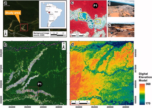
Our study area is located in Madre de Dios, a region in the southeast of Peru (see Figure 1). Madre de Dios has a flat topography, with a minimum and maximum altitude of 170 and 360 masl (meters above sea level). This moderate slope facilitates the co-registration process between optical and SAR images. The study area is included in path/row 003/069 within the World Reference System-2 (WRS-2) and covers approximately 1100 × 1100 Landsat pixels (i.e., $\approx$1090 km²). Madre de Dios is a hotspot of great biodiversity (Tarazona and Miyasiro-López 2020) and 40% of its area is protected by a set of Protected Natural Areas and Native Communities. It also has the largest coal reserves in the world (Baccini et al. 2012). However, deforestation that occurs in the region, based mainly on logging, agriculture, and gold mining (Figure 1c), is endangering forest ecosystem services and having negative effects on the surrounding population and the Peruvian state. In fact, the latest reports of deforestation, made by the Peruvian state through the national reports of the Ministry of the Environment of Peru (MINAM), indicate an increase in deforestation in recent years.

Figure 1. Political map (panel (a)) and Madre de Dios study area with a Landsat 8 OLI background image in RGB combination: SWIR2, SWIR1 and GREEN bands (panel (b)). Panel (d) shows the Digital Elevation Model (DEM) of the Shuttle Radar Topographic Mission (SRTM), both panel (b) and panel (d) represent the same study area. Panel (c) shows gold mining through PlanetLabs images (at 5 m); in addition, the resolution of this image makes it possible to see the characteristics of the gold mining in the study region (i.e., presence of water bodies).

Data and methods

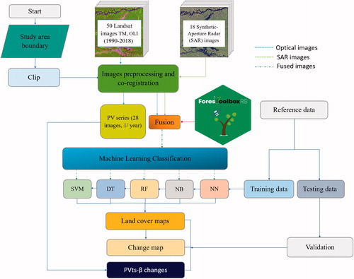
We follow a series of rigorous processes according to the premise set out in the introduction (see Figure 2). Section “Satellite image processing” details the pre-processing of optical images with the CLASlite software to obtain the PV fractions and a standard pre-processing of the SAR images that includes co-registration with optical images. Section “Deforestation reference data” provides a review of the reference data used to evaluate the obtained maps. In Section “Fusion of SAR and optical images through PCA” we conducted a brief and highly focused review of the optical and SAR data fusion method used. Finally, in Section “Mapping deforestation” we include several techniques and standard guidelines for the mapping and validation of the changing cartography.

Figure 2. Flowchart of the pre-processing and processing of the optical and SAR images is shown.

Satellite image processing

Landsat data and fraction indices

In this study, 50 images from Landsat TM and OLI pairs between 1990 and 2018 with a Tier 1 processing level (Young et al. 2017) were selected. Exactly 38 images correspond to the TM sensor (1990–2011) and 12 to the OLI sensor (2013–2018). Photosynthetic Vegetation fractions were obtained from 50 reflectance images with the CLASlite software (Asner et al. 2009). In short, CLASlite uses the physical model Spectral Mixture Analysis (SMA) to obtain the PV fractions. SMA assumes that the energy received within the field of vision of the remote sensor can be considered as the sum of the energies received from each dominant endmember (specifically a Linear Mixing Model). Therefore, we would expect advantages in the detections because we are working with changes in photosynthetic activity at the subpixel level. Given the potential of CLASlite subpixel analysis, the AutoMCU approach has been widely used to map forest disturbance and deforestation worldwide (e.g., Asner et al. 2005, 2009; Carlson et al. 2012; Allnutt et al. 2013; Bryan et al. 2013; Dlamini 2017; Tarazona et al. 2018).

After obtaining the PV fractions we deal with the atmospheric artifacts using the Function of mask (Fmask) (Zhu and Woodcock 2012) to mask clouds and cloud shadows. Subsequently, and to generate cloud-free mosaics for each year, we used the algorithm proposed by Tarazona et al. (2018). This algorithm consists of three steps: (i) it chooses the image less affected by atmospheric noise, retaining the image with the highest number of clear pixels and its acquisition time, (ii) it calculates the distances (i.e., differences in acquisition time) of the image selected in step (i) to the remaining images, and (iii) it takes the clean pixels of the images, starting with the image that has the shortest distance to the image selected in step (i) and ending with the image most temporally distant.

A total of 28 yearly PV fraction images was created (1990–2018 time series) (of a total of 50 images).

ALOS PALSAR and Sentinel-1 data

We used ALOS PALSAR data in Fine Beam Dual Polarization (FBD) with Terrain Corrected for this study. The image was acquired on August 12th, 2009, with a spatial resolution of 12.5 m, a swath of 70 km, in HH and HV-polarizations. Both polarizations were acquired in gamma-naught radar backscattering coefficients (${\gamma }^0$) (Rosenqvist et al. 2007). We softened the salt and pepper effect by using a Simple Speckle Filter (SSF) through the Lee filter (Lee 1980) with a movable 3 × 3 window. We then converted it into decibels (dB) using the SNAP software (Sentinel Application Platform, see http://step.esa.int/main/download/) of the European Space Agency.

Sentinel-1 is a C-band Synthetic Aperture Radar (5.5 cm wavelength) imaging mission (Torres et al. 2012) that supports a wide variety of applications, including deforestation assessment. Sentinel-1B with VV + VH polarization (S1B-VV + VH) data were acquired in Interferometric Wide Swath mode (IW with a 250 km² swath). The S1B-VH + VV image was acquired on December 22nd, 2018, and was downloaded in Ground Range Detected (GRD) format. The pre-processing was also performed with the SNAP software and consisted of three steps: (i) calibration, (ii) terrain correction, and (iii) smoothing of speckle-noise just as we did with ALOS PALSAR. For terrain correction, we used the Range-Doppler Terrain Correction model and a three arc-second DEM obtained from the SRTM and downloaded automatically by the SNAP software. The spatial output resolution after applying the correction to the terrain was 10 m. The VV and VH radar backscattering coefficients (σ0 in dB) were obtained from digital number (DN) values through Eq. (1)(1) $${dB}_{i,j}=10\times {\log }_{10}({{DN}_{i,j}}^2/A^2)$$(1) : (1) $${dB}_{i,j}=10\times {\log }_{10}({{DN}_{i,j}}^2/A^2)$$(1) where, i, j represents the position (row and column), and A represents the calibration factor, which can be looked up in the sigma naught values in the lookup table (LUT).

In addition, accurate multi-temporal co-registration is an essential prerequisite for change detection and was also carried out with the SNAP software. The Optical Landsat (see Section “Fusion of SAR and optical images through PCA”) image was selected as master and the SAR images as slaves, and a Root Mean Square Error (RMSE) accuracy threshold of 0.5 pixels was applied (i.e., 15 m). The RMSE of the co-registration between the optical and SAR images for the two periods was less than 0.5 pixels (Table 1).

Table 1. Number of tie points, threshold of accuracy and RMSE in pixel units obtained after co-registration between optical and radar data.

Fusion		Tie points	RMSE mean	RMSE std
2009	SWIR1 (master) + HH (slave)	457	0.18167	0.09060
	SWIR1 (master) + HV (slave)	489	0.16986	0.07929
2018	SWIR1 (master) + VV (slave)	568	0.24612	0.11843
	SWIR1 (master) + VH (slave)	566	0.24455	0.11167

std: standard deviation.

Deforestation reference data

In order to validate the detected deforestation events, two sources have been used as reference data (i.e., deforested areas and intact forest masks). First, we used the official deforestation reports from the Peruvian government carried out by the Ministry of the Environment (MINAM 2015) (see: http://geobosques.minam.gob.pe/geobosque/view/index.php for more details). The methodology of these reports is based on the work of Hansen et al. (2008) and Potapov et al. (2011). These reports show the deforestation between 2001 and 2017. Second, we used the global forest change data from Hansen et al. (2013), which were obtained from time-series analysis of Landsat images including the OLI sensor. These reports are open-access and are usually used as ground truth (global forest change between 2000 and 2018). We used the Google Earth Engine platform (Gorelick et al. 2017) to download them (see: https://earthenginepartners.appspot.com/science-2013-global-forest/download_v1.6.html for more details).

Fusion of SAR and optical images through PCA

To fuze optical (Landsat imagery) and SAR images (ALOS PALSAR and Sentinel-1) we used the PCA method that is widely known by the scientific community (e.g., Pereira et al. 2013; Werner et al. 2014; Abdikan 2016). The goal is to reduce the dimensionality through linear combinations of the original variables, obtaining the contribution of the optical bands and SAR in the principal components (PC). We believe that a description of the mathematical depth of the PCA is important for understanding the internal process of fusion of the two images with different observation geometries and which few studies have been able to develop; therefore, we present the mathematical description in Appendix A.

A total of nine variables ($Z_i$) are considered in the two periods. Specifically, six optical bands for both 2009 and 2018, two HH and HV polarizations for 2009, and another two VV and VH polarizations for 2018. In addition, we include the HH/HV and VV/VH ratios for 2009 and 2018, respectively. The two ratios are effective in detecting deforestation and are correlated with forest phenology (e.g., Zeng et al. 2014 and Frison et al. 2018).

The Landsat images used for the fusion were selected to match the acquisition date of the SAR images as closely as possible. Therefore, August 28, 2009 and September 6, 2018 were selected from among the available optical images. To fuze the images we used the “fusionRS” function (see Appendix B for more details). This function uses the prcomp function embedded in R (R Core Team 2020) to execute the PCA. The outputs of the “fusionRS” function are the eigenvalues, eigenvectors, the correlation of the variables with the PC and the contribution in percentage of each variable in each PC in a user-friendly and straightforward way (all the documentation on how to execute the function and also examples can be found in Appendix B).

Moreover, given the nature of the SAR images and optical images, all variables were centered and scaled (i.e., standardized) (Eq. (2)(2) $$Z=\frac{x-\mu }{\sigma }$$(2) ) before computing the PCA to prevent any variable from having a disproportionate influence on the PCA. (2) $$Z=\frac{x-\mu }{\sigma }$$(2) Where x is the original variable, μ is the mean, σ the standard deviation of the original variables and Z is the standardized variable.

Mapping deforestation

Non-seasonal detection approach

Time-series methods for mapping deforestation are generally classified into seasonal and non-seasonal approaches. Seasonal approaches are widely used and a variety of algorithms have been proposed (e.g., those proposed by Verbesselt et al. 2012 or Zhu and Woodcock 2014), but all of them are highly dependent on the seasonal component of the time series. As a result of this dependence, they have a number of shortcomings that make it difficult to map changes in the forest quickly and accurately. However, the non-seasonal approach (e.g., PVts-β proposed by Tarazona et al. (2018)), does not depend on seasonality and detections may be more accurate than the others.

Therefore, we used the PVts-β approach proposed to detect deforestation between 2009 and 2018. For this, we used series of PV fractions to minimize the effect of seasonality and improve detection accuracy. This approach consists of a series of processes that are detailed in the work of Tarazona et al. (2018). The optimal threshold values (β) (Eq. 3(3) $$L_{i,j}={\mu }_{i,j}-\beta \times {\sigma }_{i,j}$$(3) ) are 5 and 6 for PV series. In this work we used the value β = 5. (3) $$L_{i,j}={\mu }_{i,j}-\beta \times {\sigma }_{i,j}$$(3) Where, $L_{i,j}$ is the lower limit, ${\mu }_{i,j}$ is the mean, ${\sigma }_{i,j}$ is the standard deviation, $\beta$ is the threshold magnitude and $i,j$ is the row and column position of a given pixel.

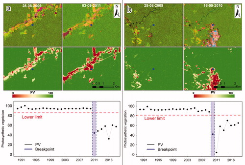
For example, Figure 3 shows two time series of the PV fraction for pixels where the forest is deforested. Figure 3a shows a deforestation event due to agricultural activity in 2011, and Figure 3b shows another deforested area in 2010, caused by gold mining activity, which has a large negative impact on the environment.

Figure 3. Examples of time series of forests that have been deforested (points in blue). The Landsat images in the top row are in combination SWIR2, NIR and RED. The middle row contains the PV fractions scaled between 0 and 100. Finally, the lower row shows the detections made by the PVts-β approach with β = 5. The PV series were smoothed, before detecting deforestation, with the “smootH” function (see Appendix B).

Classification methods

After applying PCA to fuze the images, five popular robust machine learning algorithms in the R language were used to detect changes. Support Vector Machine (SVM) was the first algorithm used. The SVM classifier is a supervised non-parametric statistical learning technique that does not assume a preliminary distribution of input data (Mountrakis et al. 2011; Pôssa and Maillard 2018). Its discrimination criterion is a hyperplane that separates the classes in the multidimensional space in which the samples that have established the same classes are located, generally some training areas. The SVM classifier has been efficiently used for mapping vegetation and forest (Knorn et al. 2009; Duro et al. 2012). The second algorithm used was Random Forest (RF). RF is a derivative of Decision Tree which provides an improvement over DT to overcome the weaknesses of a single DT (Pal 2005; He et al. 2017; Vlachopoulos et al. 2020). The prediction model of the RF classifier only requires two parameters to be identified: the number of classification trees desired, known as “ntree,” and the number of prediction variables, known as “mtry,” used in each node to make the tree grow (Rodriguez-Galiano et al. 2012). The third algorithm used was Decision Tree (DT). DT is also a supervised non-parametric statistical learning technique, where the input data is divided recursively into branches (Chen et al. 2018) depending on certain decision thresholds until the data are segmented into homogeneous subgroups. This technique has substantial advantages for remote sensing classification problems due to its flexibility, intuitive simplicity, and computational efficiency (Friedl and Brodley 1997). The fourth algorithm used was Naive Bayes (NB). The NB classifier is an effective and simple method for image classification based on probability theory. The NB classifier assumes an underlying probabilistic model and captures the uncertainty about the model in a principled way, that is, by calculating the occurrence probabilities of different attribute values for different classes in a training set (Pradhan et al. 2010). The last algorithm used was Neuronal Networks (NN). This classification consists of a neural network that is organized into several layers, that is, an input layer of predictor variables, one or more layers of hidden nodes, in which each node represents an activation function acting on a weighted input of the previous layers’ outputs, and an output layer (Liu et al. 2019).

The fine-tuning of model hyperparameters can significantly increase the target in both training and testing; however, it also increases the cost of training models and the risk of overfitting. Therefore, in this research, we decided to use the default parameters (see S1 in supplementary material) after examining a large number of studies (Belgiu and Drăguţ 2016; Tyralis et al. 2019; Zurqani et al. 2019).

Since our study area is located in the Amazon, obviously the classes to be identified were mainly forest, cropland, bare soil, and water. Classification of crop types or differentiating secondary forests from virgin forests will not be addressed in this study due to the nature and objectives of the research. The objective is to separate the forest from other classes.

Calibration

Undoubtedly, given a large number of machine learning algorithms, it was necessary to select the one with the best performance in the classification, that is, the algorithm in which the training and testing data used converge the learning iteratively to a solution that appears to be satisfactory. Therefore, calibration at this stage was crucial and was carried out through Cross-Validation (CV) and Monte Carlo Cross-Validation (MCCV). We used k groups equal to 10 (10 iteration) and an iteration equal to 100 for CV and MCCV respectively. In order to select the best classifier, which will then serve as input for the 2009 and 2018 classifications, it was necessary to minimize the testing bias (the mean of errors $e_i=1-\text{overall accuracy}$) (Eq. (4)(4) $$\mathrm{Bias}={\sum }_{i=1}^n{e}_i/n$$(4) ) and the testing variance (the standard deviation of errors e_i) (Eq. (5)(5) $$\mathrm{Variance}=\sqrt{{\sum }_{i=1}^n{(e_i-\underset{\_}{e})}^2/n}$$(5) ) so that the model works well for both the training data and the test data. This process and analysis were written in R with the help of some libraries, such as caret and willcoxCV. (4) $$\mathrm{Bias}={\sum }_{i=1}^n{e}_i/n$$(4) (5) $$\mathrm{Variance}=\sqrt{{\sum }_{i=1}^n{(e_i-\underset{\_}{e})}^2/n}$$(5) Where $i$ represents the position of a specific iteration and $n$ represents the total number of iterations executed.

Accuracy assessment and map comparison

A total of 1670 training points were taken to calibrate and validate the different cartographic products generated (Table 2). These points were selected through the interpretation of the satellite images themselves, truth-terrain reference data elaborated by MINAM (2015) and, on some occasions, we used high-resolution images such as Google Earth. First, we selected 560 points for the calibration of the five classifiers for each of the two years, 2009 and 2018, through a stratified random sampling approach (Olofsson et al. 2014). These same points were also used to obtain the definitive 2009 and 2018 class maps using the classifier with the best performance. In both periods, the 560 points were split into training (60%) and testing (40%) sets through proportional stratified random sampling. Finally, to validate the change map generated with the classifiers and the changes with the PVts-β approach, we selected 550 points using stratified random sampling (80% for intact forest and the rest for deforested areas).

Table 2. Number of points for the calibration of the classifiers and also for obtaining the change cartography for the years 2009 and 2018, as well as samples for validating the changes obtained with the classifiers and the PVts-β approach.

	Calibration		Change validation
	Year 2009	Year 2018
Classifiers
Forest	225	225	Training
Cropland	125	125	336
Bare soil	105	105	Testing
Water	105	105	224
Total	560	560	560
Change maps			550
PVts-β approach

To evaluate the accuracy of both the image fusion classifications and the detections of the PVts-β approach, we used indicators such as overall accuracy, user’s accuracy, producer’s accuracy, and kappa index (Congalton and Green 2008). These indicators have been widely discussed and used in a large number of papers, such as Schultz et al. (2016) and Duro et al. (2012), among others.

Results

Fusion of optical and SAR images

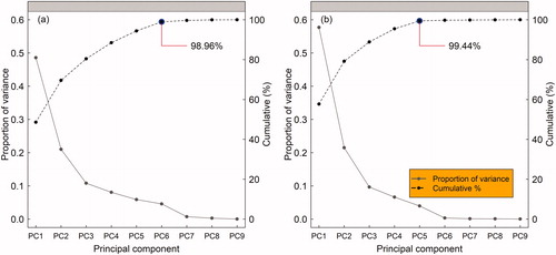
The fusions of optical and SAR data for the years 2009 and 2018 are shown in Figure 4a–h. In both panels, they are shown in a 1-2-3 combination of 9 principal components (Figure 4i–j). Only the first principal components provided the greatest variance in explaining the data in both 2009 and 2018 (Figure 5). At this stage we used the jambu elbow (Tibshirani et al. 2001) to decide which components to take out of the equation due to the poor contribution to the variance. In fact, for 2009 and 2018, only the six and five principal components had an accumulated variance of 98.96% and 99.44% respectively (Figure 5). In addition, increasing the number of principal components would bring us closer to a context of using almost all the variables involved and an increase in noise, which could ultimately hinder the classification process through automatic learning algorithms.

Figure 4. Panel (a) and (b) show the combinations NIR, RED and GREEN and SWIR2, SWIR1, GREEN from the year 2009 (Landsat-5 TM). Panel (c) and (d) show the same region with polarizations HH and HV (ALOS PALSAR—2009) respectively. Panel (e) and (f) show the combinations NIR, RED and GREEN and SWIR2, SWIR1, GREEN from the year 2018 (Landsat-8 OLI). Panel (g) and (h) show the same region with polarizations VV and VH (Sentinel 1B—2018). Finally, panel (i) and (j) show the fused images of 2009 and 2018 respectively, in both cases using a combination with the first three principal components.

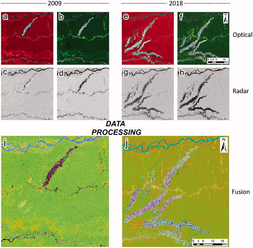
Figure 5. Proportion of variance of each PC and the cumulative variance for the year 2009 is shown in panel (a); panel (b) shows the same for the year 2018.

On the other hand, Table 3 shows the contributions (%) of the original variables to the principal components. In general, for the year 2009 almost all optical bands had a significant contribution in PC1 (except NIR band), the NIR and SWIR1 bands in PC2:3, all bands in PC4 (except SWIR2), all (except RED and NIR bands) in PC5 and the NIR, SWIR1 and SWIR2 bands in PC6. While all polarizations had a strong contribution in all PC1:6 (except HH in PC1, HH/HV in PC2 and PC6, HV in PC3 and HH in PC6). In addition, it is important to note that, of all the SAR bands, the HV polarization had the largest contribution in PC1, followed by HH/HV. For 2018, the behavior is quite similar. Like 2009, almost all optical bands made a large contribution in PC1 (except NIR band), NIR, SWIR1 and SWIR2 bands in PC2, RED, NIR and SWIR1 in PC3, all bands in PC4 and all bands (except SWIR1 and SWIR2) in PC5. While all polarizations, especially VH and VV, had a significant contribution in PC1:5, with the exception of PC4.

Table 3. Contribution in percentages (%) of the variables to the principal components after the fusion of optical and SAR images for the years 2009 and 2018.

	Contributions (%)
	Year 2009
	PC1	PC2	PC3	PC4	PC5	PC6	PC7	PC8	PC9
Proportion of variance (%)	48.601	21.013	10.806	8.067	5.890	4.579	0.722	0.286	0.035
BLUE	20.017	0.641	0.053	7.611	2.763	5.132	56.201	0.000	7.945
GREEN	21.138	0.204	0.061	6.675	2.370	2.780	2.486	1.194	63.212
RED	20.618	1.015	0.369	7.844	1.656	0.183	38.885	1.498	28.332
NIR	0.409	34.911	8.292	7.437	1.304	37.021	1.351	8.363	0.344
SWIR1	9.507	17.939	3.343	8.973	5.077	10.057	0.984	42.521	0.058
SWIR2	17.963	1.647	0.208	0.574	4.488	27.996	0.009	46.417	0.106
HH	1.725	18.939	35.887	15.133	27.235	2.118	0.002	0.001	0.000
HV	5.402	23.393	2.858	5.995	49.887	14.039	0.078	0.000	0.000
HH/HV	3.216	1.305	48.925	39.755	5.216	0.670	0.000	0.002	0.000
	Year 2018
Proportion of variance (%)	57.723	21.485	9.650	6.618	3.964	0.339	0.103	0.089	0.029
BLUE	16.698	0.772	1.568	8.781	9.807	53.780	0.200	0.001	8.389
GREEN	17.618	0.375	1.715	5.779	7.148	2.609	0.018	1.728	63.006
RED	17.816	0.125	2.151	2.780	6.491	41.863	0.163	0.547	28.058
NIR	0.382	28.121	17.701	40.529	11.477	0.547	0.117	1.100	0.021
SWIR1	7.373	22.559	4.034	22.293	2.661	0.388	3.596	36.929	0.163
SWIR2	12.684	11.431	0.357	18.788	0.110	0.008	3.052	53.207	0.358
VV	11.513	16.100	5.491	0.220	10.170	0.094	52.850	3.555	0.001
VH	12.173	5.548	9.535	0.500	48.260	0.590	21.554	1.835	0.001
VV/VH	3.737	14.965	57.444	0.325	3.871	0.116	18.446	1.093	0.000

Lower contributions in each PC are shown in red and blue for optical and radar bands respectively. The last PC that will not be used in the classification are shown in gray.

Algorithm calibrations

From a series of five automatic learning algorithms, the idea was to select the classifier that meets two conditions: (i) high overall accuracy and (ii) best performance in predicting the forest and cropland categories within the validation data.

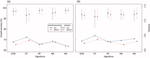
The bias and variance of the calibration of the classifiers had notable differences with CV and MCCV (Figure 6). That is, calibrations with CV had a slightly greater variance than calibrations with MCCV, mainly because CV only explores some of the possible ways in which data could have been partitioned (e.g., testing and training). In fact, MCCV allowed 90 times more exploration of possible partitions from a total of $C_{560}^{280}\approx \mathrm{\infty }.$ In short, the calibrations indicated that the algorithms with the best performance in overall accuracy and the lowest variance were SVM, NN, and RF (overall average accuracy of 97.50% and 98.00% with CV and MCCV respectively) for 2009 and NN (overall average accuracy of 93.93% and 94.80% with CV and MCCV, respectively) for 2018 (Figure 6). However, all classifiers had an acceptable overall accuracy greater than 90%. In both periods, the classifier with the lowest overall average accuracy was DT.

Figure 6. The calibrations were performed through CV and MCCV, panel (a) is for the year 2009 and panel (b) is for the year 2018. The minimum, maximum and average of the overall accuracies for each algorithm are shown. In addition, we show the variance obtained for the k = 10 groups and for 100 iterations.

Visual examination of thematic maps

Since the objective is to quantify deforestation, it is very important that the algorithm optimally discriminates the forest from other types of cover. Figures 7 and 8 show the thematic maps obtained by the five classifiers in 2009 and 2018 respectively. In both periods, especially in 2009, the visual interpretation between the thematic maps obtained by the five classifiers revealed an erroneous amount of the cropland class represented in the extreme north and southwest of the study area. In fact, a visual inspection of the Landsat images and high-resolution PlanetLabs images revealed that these areas are predominantly covered by forests. However, there is also a certain level of deforestation in these areas, which could have led to confusion between forest and cropland classes.

Figure 7. Classifications using the six principal components of the fused image in the year 2009. Panels (a), (b), (c)*, (d) and (e) represent the classifications obtained with SVM, DT, RF (*the highest overall accuracy), NB and NN, respectively.

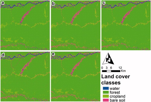
Figure 8. Classifications using the five principal components of the fused image in the year 2018. Panels (a), (b), (c), (d) and (e)* represent the classifications obtained with SVM, DT, RF, NB, and NN (*the highest overall accuracy) respectively. Class “Difference*” represents the difference map of the same classifier between 2009 and 2018 with ground truth (Hansen et al. 2013).

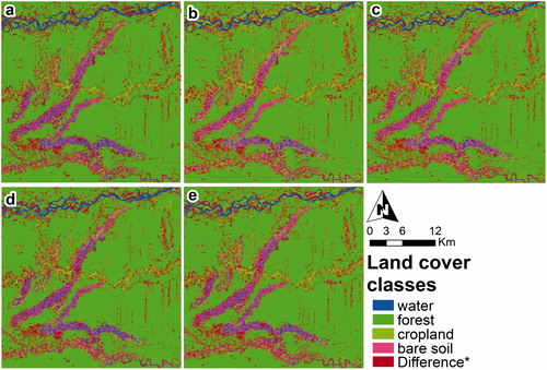
In general, all algorithms produced reasonably accurate land cover maps in both study periods. Nevertheless, the results of the RF algorithm in 2009 and NN in 2018 were of special interest as they show a better performance in separating forest and cropland cover with low omission and commission levels, and with an overall accuracy of 95.09% in both years (Table 4). A more detailed analysis showed that the average commission for the forest class in 2009 was 0.33% higher than in 2018, and the average omission for the same class in 2009 was 2.86% lower than in 2018. However, the “salt and pepper” effect was present in both periods, especially in 2018 for the classifiers NB, DT, and NN (Figures 7 and 8).

Table 4. Overall accuracy and Kappa index for all classification algorithms and both dates.

	Overall Accuracy	Kappa Index	Water		Forest		Cropland		Bare soil
			OM	CO	OM	CO	OM	CO	OM	CO
2009
SVM	95.09	93.07	0.00	0.00	0.00	9.00	22.22	2.78	2.44	2.44
DT	93.30	90.55	2.13	0.00	1.10	10.0	26.67	8.33	2.44	4.76
RF	95.09	93.11	2.13	0.00	1.10	6.25	17.78	5.13	2.44	6.98
NB	93.30	90.58	2.13	0.00	2.20	9.18	24.44	10.53	2.44	4.76
NN	95.09	93.09	0.00	0.00	1.09	8.16	20.00	5.26	2.44	2.44
2018
SVM	94.20	91.94	0.00	4.65	2.33	9.68	20.37	4.44	0.00	0.00
DT	92.86	90.12	0.00	10.87	3.49	6.74	20.37	10.42	4.65	0.00
RF	94.64	92.58	0.00	0.00	4.65	7.87	12.96	9.62	2.33	0.00
NB	93.75	91.38	0.00	4.65	6.98	6.98	14.82	11.54	0.00	0.00
NN	95.09	93.18	0.00	0.00	2.33	9.68	16.67	4.25	0.00	0.00

Omission errors (OM) and commission errors (CO) are also shown. All values are in percentages (%). For overall accuracy, the highest values for each date are shown in bold, as well as lower commission and omission errors in the forest and cropland categories. The green background indicates the best classifier for each year, selected to maximize overall accuracy as well as minimize omission and commission errors for forest and cropland areas. See S2 in the supplementary material for more details.

Change validation and statistical comparisons

Figure 9 shows deforestation areas obtained with the PVts-β approach, the RF-NN classifiers (i.e., changes obtained using the RF and NN classifiers) and the reference data. Visually, the detections of the PVts-β approach (Figure 9a) and the RF-NN algorithms (Figure 9b) reveal a lot of similarity with the reference data of Hansen et al. (2013) (Figure 9c) and the MINAM reports (Figure 9d), although a closer inspection showed some visual differences between the two detection methods, mainly south of the study region (i.e., in elliptical white line). That is, a compact and continuous quantification should be expected. However, only the change obtained by the RF-NN classifiers shows something more detectable and logical (i.e., detection of deforestation in areas of gold activity should include not only the bare soil but also the water bodies in the areas).

Figure 9. Panel (a) and (b) show deforestation detections (2009–2018) obtained from the PVts-β approach and the RF-NN classifiers respectively. Panel (c) and (d) show the reference data from Hansen et al. (2013) and MINAM respectively. All the panels have the SWIR1, NIR and RED combination from the year 2018 (Landsat 8 OLI) as the background.

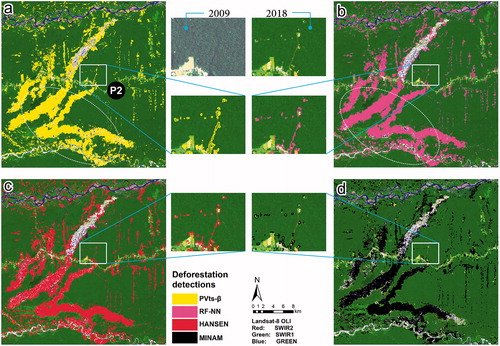
However, the change maps showed that the overall accuracy obtained with the PVts-β approach was 92.91%. This was higher by 1.09% than the overall accuracy obtained with the RF-NN classifiers (Table 5). In addition, the lowest omissions and commissions were obtained with the PVts-β approach and RF-NN classifiers with 9.85% and 9.98% respectively. Visual analysis revealed that the commission of the PVts-β approach was mainly in gold mining areas, while the omission was in agricultural and gold mining areas, which were not optimally detected. Moreover, for a rigorous statistical comparative analysis, a forest/non-forest mask of the reference data from Hansen et al. (2013) was used to eliminate commissions from detection approaches. The statistics revealed that there was no significant difference between the mapped areas with respect to the reference data. In fact, both the PVts-β approach and the RF-NN algorithms detected a total of 18142.74 ha and 16276.05 ha respectively, while the reference data from Hansen et al. (2013) recorded 19708.35 ha between 2009 and 2018. For the period 2009–2017, the PVts-β approach detected 15998.31 ha, while Hansen et al. (2013) and MINAM reference data reported 16903.89 ha and 17877.15 ha respectively. Finally, from the changes obtained with the RF-NN classifiers, it is important to mention that between 2009 and 2018 the forests mainly changed to cropland 7169.49 ha, bare soil 4507.56 ha, and water 4599.00 ha.

Table 5. Overall accuracy, kappa index, and the average commission and omission errors (average commissions and omissions from deforestation classes and intact forest) are shown for the PVts-β approach, and for the change obtained with the RF-NN classifiers.

	Overall accuracy	Kappa index	Commission	Omission
PVts-β approach	92.91	78.36	11.67	9.85
Change with RF-NN	91.82	72.26	9.98	16.7

All values are in percentages (%).

Discussion

As expected, image fusion showed that the HV and VH cross-polarizations had a slightly greater contribution than the HH and VV polarizations in PC1 (Table 3). In general, for the year 2009, it is observed that almost all the radar bands made a significant contribution to PC2:5, while for the year 2018, the highest radar contributions were observed in PC1:5 (except in PC4). In addition, the NIR band (a representative optical band for vegetation mapping) made a lower contribution than any other optical band in PC1 (even lower than the radar bands) in both study periods. However, this was not the case with the RED band. On the other hand, the vegetation structure (Shimada et al. 2014) and the detection of non-photosynthetic activity (e.g., fallen leaves) due to the penetration of ALOS PALSAR images, probably made it possible to map the forest class optimally in 2009 (see omission in Table 4).

To explore the performance of image fusion in detections, we detected changes only with optical images. These detections were underestimated by 2660 ha with respect to the fused images, which is shown in S3 in the supplementary material. We believe that the difference between what is detected with fused images and optical images is relatively small but it is an indicator that the fusion of optical and radar data contributes to the mapping of deforestation.

To analyze whether speckle noise and feature resolution had any influence on change detection, we decided to apply a Multi-temporal Speckle Filter (MSF) (Quegan and Yu 2001) to the SAR images before fusing with the optical data. For the year 2009, we obtained HH, HV, and HH/HV polarizations from a total of 7 ALOS PALSAR images; while for the year 2018, we obtained VV, VH, and VV/VH polarizations from a total of 11 S1B images (see S4 in the Supplementary material). The change map showed deforestation of 16132.77 ha between 2009 and 2018 (in both periods, we used PC1:6 ≈ 99% of cumulative variance) using the algorithms that performed best in the calibrations, that is, RF in 2009 as well as 2018. Although MSF resulted in sharper and clearer boundaries (Figure 10a–c in yellow and red lines), SSF together with optical data quantified the deforestation better. Similar results were obtained in the study by Mirelva and Nagasawa (2017) (although these authors only worked with radar data). Overall, no substantial differences were found between the two filter types (Figure 10d, panels 3 and 4, Table 6), although for the areas with higher signal echo intensity the SSF filter performed better. In addition, the MSF seems to have an effect on the contribution of the SAR bands to the first PC, since lower contributions were observed with respect to SAR bands with SSF (see Table 3 and Table S4 for more details).

Figure 10. Column (a) shows SAR images without a speckle filter, column (b) images with SSF, column (c) shows a Multi-temporal Speckle Filter (MSF). To evaluate the reduction of speckle noise we used three indicators: (i) visual interpretation, (ii) Signal Level Ratio (SLR) (White et al. 2020), and (iii) the standard deviation of the intensity before and after applying filters for areas with higher signal echo intensity (P3) and areas with lower signal echo intensity (P4) (column d). The parameters for the MSF filter were used by default: (i) filter: filter Lee, (ii) Number of looks: 1, (iii) Window size: 7 × 7, and (iv) Sigma: 0.9.

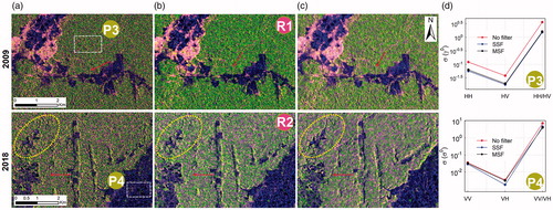
Table 6. SLR is a ratio of the unfiltered image to the filtered image averaged over a region (R1 and R2).

	Mean			SLR
	RAW	SSF	MSF	SSF	MSF
R1
HH	0.2139	0.2140	0.2130	0.9995	1.0042
HV	0.0642	0.0642	0.0640	1.0000	1.0031
R2
VV	0.1417	0.1414	0.1774	1.0021	0.7988
VH	0.0331	0.0331	0.0390	1.0000	0.8487

A mean of one indicates that the filtered image preserves the signal level accurately. If the mean varies from one, then there is a bias in the filtering method.

Although the classifications obtained with the five classifiers performed well in overall accuracy, they all had confusions between forest and cropland. This is mainly due to the similarity of the spectral response of the two coverages, predominantly in the optical electromagnetic spectrum. In these situations an increase in the number of variables, for example, vegetation indices or other images from different dates, improves the separability of certain relatively confusing covers and slightly improves the overall accuracy of the classification, but does not detect deforestation better, as can be seen in section S5 on the supplementary material.

Another aspect that needs to be discussed is the presence of “salt and pepper” in all the classifications obtained, although much less in the period 2009. In general, SVM revealed a lower proportion of this type of noise in the two study periods. It is not clear whether the speckle noise of the SAR images was the main origin of the “salt and pepper” since Duro et al. (2012), who analyzed optical images, also obtained similar results to ours with classifications contaminated by this type of noise in several algorithms of machine learning, although in a smaller proportion, by classifiers like SVM and RF. In addition, the study area is a region with very particular characteristics and it is a challenge to map deforestation since the areas deforested by gold mining trigger not only the presence of bare soil (i.e., sand) but also water bodies (Figure 1c). This is a product of the activity itself which hinders certain pre-processing methods such as masking of atmospheric noise in optical images (Tarazona et al. 2018). That is, the masking of atmospheric noise could mask areas that are deforested by mining activity. Therefore, the quantification of deforestation would reveal a certain degree of omission. This is clearly seen in the quantifications (yellow lines) carried out with the PVts-β approach and the reference data, but not so much with the quantifications carried out with the RF-NN classifiers (see Figure 9). This difficulty is not present in the SAR images (this can be seen in the detection of fusion), where water bodies resulting from gold mining are recorded with low backscatter values (see white lines in Figure 9b).

Another important point of discussion is the detection threshold of the PVts-β approach, since the omission of the detections occurred mainly in agricultural coverages. To avoid this deficiency, it is possible to lower the threshold to β = 3; however, this could trigger a slight increase in the commission. In any case, for future work, it will be important to assess to what extent a threshold of β = 3 can increase commission levels, although the latter is possible to combat with a forest/non-forest mask.

Finally, according to this work’s context, it is important to make an analysis of the detection approaches based on time series and those based on machine learning. Each approach has advantages and disadvantages in certain aspects. For example, it is clear that a machine learning approach, in contrast to a time series approach, is unlikely to detect slight changes over time in photosynthetic activity. However, if the atmospheric noise and seasonality of the time series are not eliminated or minimized correctly, it could make any further analysis in the time series difficult. On the other hand, the machine learning approach has the advantage from a computational and execution point of view (see S6 in the supplementary material). Furthermore, the main global deforestation mapping methodologies are based on classifications such as Hansen et al. (2013), Hansen et al. (2016), and Asner et al. 2009 (CLASlite), although lately, thanks to the GEE platform (Gorelick et al. 2017), there have been efforts to implement detections based on time series, such as the LandTrendr method (Kennedy et al. 2010), which is embedded in GEE (https://emapr.github.io/LT-GEE/). However, most detection methods based on time series have: (i) excessive calibration parameters, (ii) are based strongly on seasonality, and (iii) are complex to execute for a standard user. On the other hand, the PVts-β approach is a method that: (i) is simple and intuitive and which does not model seasonality, (ii) has only one calibration parameter to detect deforestation, and iii) can be easily implemented by any standard user.

Conclusions

Fusing optical and SAR data has been studied at length in the past, but the contribution (%) of each of the original variables within the fusion has not been addressed optimally. This research shows the benefits of combining optical and SAR data for detecting deforestation compared to using only optical data. The contribution of SAR bands, especially HV, HH/HV, VH, and VV, was substantially important in both study periods. We believe that the benefits can be greater if the SAR images have been acquired after the optical images since in areas of high precipitation cloud-free optical images are usually only available between June and September. Therefore, when only optical images are used there is a void of three months with no record of the changes in the forest. Regarding speckle noise, although MSF better preserves the characteristics of the entities (better “spatial resolution”), it seems to decrease the contributions (unlike SSF) of the SAR bands in the data fusion and underestimates the detection of deforestation. In addition, there were no significant differences between the backscatter values obtained after applying MSF and SSF filters. However, the calibration of the machine learning algorithms revealed that all classifiers had an acceptable overall accuracy. In fact, all classifications had an overall accuracy of more than 90%.

The overall accuracy of the PVts-β and RF-NN detections was very similar, although the highest commission and lowest omission were obtained with the PVts-β approach. We believe that this approach is a simple and intuitive detection method. Moreover, it can be applied to images that come from different sensors with dissimilar periodicity because it does not depend on the seasonality of the data (i.e., correlated data). In addition, it is important that the data set is large enough (>5 data) to avoid bias in the calculation of the mean and standard deviation.

Finally, given the increased interest and activity in simple, effective, and low-cost forest monitoring methods, PVts-β is clearly a strategic tool. Therefore, the PVts-β approach, the algorithm for fusing optical and radar data and other functions is implemented in an open-source package called “ForesToolboxRS” (see Appendix B for more details).

Acknowledgments

The work of Yonatan Tarazona Coronel has been partially funded by American Program in GIS and Remote Sensing and National Program of Scholarships and Educational Credit (PRONABEC–Peru) through RJ: N° 4276-2018-MINEDU/VMGI-PRONABEC-OBE and RJ: N° 942-2019-MINEDU/VMGI-PRONABEC-OBE. Xavier Pons is the recipient of an ICREA Academia Excellence in Research Grant. The GRUMETS Research Group is partially supported by the Catalan Government under Grant SGR2017-1690. This work has also been supported by the Spanish MCIU Ministry through the NEWFORLAND project (RTI2018-099397-B-C21 (MCIU/AEI/ERDF, EU)). In addition, we would especially like to thank Dr. Xin Miao for his kind and appropriate suggestions and comments, as well as different anonymous reviewers for their timely comments that improved the content of the manuscript. Finally, we thank the General Direction of Environmental Territorial Planning of the Ministry of the Environment of Peru for providing us with some data used in this work.

Disclosure statement

The authors report that there is no conflict of interest.

Appendix A

All the variables (optical and SAR) are centered and scaled, and it is a question of calculating a new set of bands ($Y_1,$ $Y_2,$…, $Y_p$) uncorrelated among themselves, whose variances progressively decrease. Each component $Y_j$ ($j=1,\mathrm{ }\dots ,\mathrm{ }p$) is a linear combination of the original variables: (1) $$Y_1=u_{11}{Z}_{1i}+u_{12}{Z}_{2i}+\cdots +u_{1\mathrm{p}}{Z}_{pi}$$(1)

In abbreviated notation we will say $Y_1=Z{u}_1$

So the variance of the first component will be: (2) $$\mathit{var}\left(Y_1\right)=\frac{1}{n}{\sum }_{i=1}^n{Y}_{1i}^2=\frac{1}{n}{Y}_1^t{Y}_1\mathrm{ }$$(2)

Eq. (1)(1) $${dB}_{i,j}=10\times {\log }_{10}({{DN}_{i,j}}^2/A^2)$$(1) in Eq. (2)(2) $$Z=\frac{x-\mu }{\sigma }$$(2) (3) $$\frac{1}{n}{u}_1^t{Z}^{t}Z{u}_1=u_1^t\left[\frac{1}{\mathrm{n}}{Z}^{t}Z\right]u_1=u_1^{t}R{u}_1\mathrm{ }$$(3)

The expression $\frac{1}{n}{Z}^{t}Z$ is the matrix of correlations (R) on standardized variables (i.e., centered and scaled) (Jolliffe 2002; James et al. 2013).

The first component $Y_1$ is obtained so that its variance is maximum, that is, it is about finding $Y_1$ maximizing $\mathit{var}\left(Y_1\right)=u_1^{t}R{u}_1$ with the restriction ${\sum }_{j=1}^p{u}_1^t{u}_1=1.$

Since the objective is to maximize a function of several variables subject to a constraint and the incognita being $u_1$ (the unknown vector that gives the optimal linear combination) we will apply the Lagrange multiplier: (4) $$L\left(u_1\right)=u_1^{t}R{u}_1-\lambda \left(u_1^t{u}_1-1\right)\mathrm{ }$$(4) and then $\frac{\partial L}{\partial u_1}$ (derive with respect to the incognita $u_1$) and equal to zero: (5) $$\frac{\partial L}{\partial u_1}=2R{u}_1-2R=0\mathrm{ }\Rightarrow \mathrm{ }\left(R-\lambda I\right)u_1=0\mathrm{ }$$(5)

Eq. (5)(5) $$\mathrm{Variance}=\sqrt{{\sum }_{i=1}^n{(e_i-\underset{\_}{e})}^2/n}$$(5) can be deduced that $\left|R-\lambda I\right|=0$ and with roots ${\lambda }_1,\mathrm{ }{\lambda }_2,\mathrm{ }\dots ,\mathrm{ }{\lambda }_n,$ ordered from highest to lowest ${\lambda }_1>{\lambda }_2>\dots >{\lambda }_n.$ On the other hand, if we multiply to the left by $u_1^t,$ we conclude that: $$u_1^t\left(R-\lambda I\right)u_1=0\mathrm{ }\Rightarrow \mathrm{ }{u}_1^{t}R{u}_1=\lambda \mathrm{ }\Rightarrow \mathrm{ }\mathit{var}\left(Y_1\right)=u_1^{t}R{u}_1=\lambda$$

To maximize the variance of $Y_1,$ we have to take the largest eigenvalues ${\lambda }_1$ and the corresponding eigenvectors $u_1,$ so that the first component is defined as $Y_1=Z{u}_1.$ Therefore, all components are expressed as the product of the matrix of eigenvectors multiplied by the vector $Z$ containing the original variables: $$Y=uZ$$

Being, $$Y=(Y_1\mathrm{ }{Y}_2\mathrm{ }⋮\mathrm{ }{Y}_p\mathrm{ })\mathrm{ }u=(u_{11}\mathrm{ }{u}_{12}\cdots u_{1p}\mathrm{ }{u}_{21}\mathrm{ }{u}_{22}\cdots u_{2p}\cdots \mathrm{\hspace{0.17em}}\cdots \mathrm{\hspace{0.17em}}\cdots \mathrm{\hspace{0.17em}}\cdots u_{p1}\mathrm{ }{u}_{p2}\cdots u_{pp})Z=(Z_1\mathrm{ }{Z}_2\mathrm{ }⋮\mathrm{ }{Z}_p\mathrm{ })\text{and }\{\mathit{var}(Y_1)={\lambda }_1\mathrm{ }\mathit{var}(Y_2)={\lambda }_2\mathrm{ }⋮\mathrm{ }\mathit{var}(Y_p)={\lambda }_p$$ With the same logic it is possible to find the eigenvalues and eigenvectors for the remaining components.

Appendix B. Code

The source code and full instructions on how to execute the functions can be found through GitHub (please see https://github.com/ytarazona/ForesToolboxRS for more details).

References

- Abdikan, S. 2016. “Exploring image fusion of ALOS/PALSAR data and LANDSAT data to differentiate forest area.” Geocarto International, Vol. 33(No. 1): 21–37. doi:https://doi.org/10.1080/10106049.2016.1222635.
- Achard, F., Beuchle, R., Mayaux, P., Stibig, H.J., Bodart, C., Brink, A., Carboni, S., et al. 2014. “Determination of tropical deforestation rates and related carbon losses from 1990 to 2010.” Global Change Biology, Vol. 20(No. 8): 2540–2554. doi:https://doi.org/10.1111/gcb.12605.
- Allnutt, T.F., Asner, G.P., Golden, C.D., and Powell, G.V.N. 2013. “Mapping recent deforestation and forest disturbance in northeastern Madagascar.” Tropical Conservation Science, Vol. 6(No. 1): 1–15. doi:https://doi.org/10.1177/194008291300600101.
- Asner, G.P., Knapp, D.E., Broadbent, E.N., Oliveira, P.J.C., Keller, M., and Silva, J.N. 2005. “Selective logging in the Brazilian Amazon.” Science, Vol. 5747: 480–482. doi:https://doi.org/10.1126/science.1118051.
- Asner, G.P., Knapp, D.E., Balaji, A., and Paez-Acosta, G. 2009. “Automated mapping of tropical deforestation and forest degradation: CLASlite.” Journal of Applied Remote Sensing, Vol. 3(No. 1): 033543. doi:https://doi.org/10.1117/1.3223675.
- Baccini, A., Goetz, S.J., Walker, W.S., Laporte, N.T., Sun, M., Sulla-Menashe, D., Hackler, J., et al. 2012. “Estimated carbon dioxide emissions from tropical deforestation improved by carbondensity maps.” Nature Climate Change, Vol. 2: 1–4. doi:https://doi.org/10.1038/nclimate1354.
- Belgiu, M., and Drăguţ, L. 2016. “Random forest in remote sensing: A review of applications and future directions.” ISPRS Journal of Photogrammetry and Remote Sensing, Vol. 114: 24–31. doi:https://doi.org/10.1016/j.isprsjprs.2016.01.011.
- Bryan, J.E., Shearman, P.L., Asner, G.P., Knapp, D.E., Aoro, G., and Lokes, B. 2013. “Extreme differences in forest degradation in Borneo: Comparing practices in Sarawak, Sabah, and Brunei.” PLoS One, Vol. 8(No. 7): e69679. doi:https://doi.org/10.1371/journal.pone.0069679.
- Carlson, K.M., Curran, L.M., Ratnasari, D., Pittman, A.M., Soares-Filho, B.S., Asner, G.P., Trigg, S.N., Gaveau, D.A., Lawrence, D., and Rodrigues, H.O. 2012. “Committed carbon emissions, deforestation, and community land conversion from oil palm plantation expansion in West Kalimantan, Indonesia.” Proceedings of the National Academy of Sciences of the United States of America, Vol. 109(No. 19): 7559–7564. doi:https://doi.org/10.1073/pnas.1200452109.
- Chen, Y., Niu, Z., Johnston, C.A., and Hu, S. 2018. “A unifying approach to classifying wetlands in the Ontonagon River Basin, Michigan, using multi-temporal Landsat-8 OLI imagery.” Canadian Journal of Remote Sensing, Vol. 44(No. 4): 373–389. doi:https://doi.org/10.1080/07038992.2018.1526065.
- Congalton, R.G., and Green, K. 2008. Assessing the Accuracy of Remotely Sensed Data, Principles and Practices. Boca Raton, FL: CRC Press.
- Ding, Y., Zang, R., Lu, X., and Huang, J. 2019. “Functional features of tropical montane rain forests along a logging intensity.” Ecological Indicators, Vol. 97: 311–318. doi:https://doi.org/10.1016/j.ecolind.2018.10.030.
- Dlamini, W.M. 2017. “Mapping forest and woodland loss in Swaziland: 1990–2015.” Remote Sensing Applications: Society and Environment, Vol. 5: 45–53. doi:https://doi.org/10.1016/j.rsase.2017.01.004.
- Duro, D.C., Franklin, S.E., and Dubé, M.G. 2012. “A comparison of pixel-based and object-based image analysis with selected machine learning algorithms for the classification of agricultural landscapes using SPOT-5 HRG imagery.” Remote Sensing of Environment, Vol. 118: 259–272. doi:https://doi.org/10.1016/j.rse.2011.11.020.
- FAO. 2018. Global Forest Resources Assessment 2020. Rome, Italy: Food and Agricultural Organization.
- Friedl, M.A., and Brodley, C.E. 1997. “Decision tree classification of land cover form remotely sensed data.” Remote Sensing of Environment, Vol. 61(No. 3): 399–409. doi:https://doi.org/10.1016/S0034-4257(97)00049-7.
- Frison, P.-L., Fruneau, B., Kmiha, S., Soudani, K., Dufrêne, E., Le Toan, T., Koleck, T., Villard, L., Mougin, E., and Rudant, J.-P. 2018. “Potential of Sentinel-1 data for monitoring temperate mixed forest phenology.” Remote Sensing, Vol. 10(No. 12): 2049. doi:https://doi.org/10.3390/rs10122049.
- Gibson, L., Lee, T.M., Koh, L.P., Brook, B.W., Gardner, T.A., Barlow, J., Peres, C.A., et al. 2011. “Primary forests are irreplaceable for sustaining tropical biodiversity.” Nature, Vol. 478(No. 7369): 378–381. doi:https://doi.org/10.1038/nature10425.
- Gorelick, N., Hancher, M., Dixon, M., Ilyushchenko, S., Thau, D., and Moore, R. 2017. “Google Earth Engine: Planetary-scale geospatial analysis for everyone.” Remote Sensing of Environment, Vol. 202: 18–27. doi:https://doi.org/10.1016/j.rse.2017.06.031.
- Hansen, M.C., Krylov, A., Tyukavina, A., Potapov, P.V., Turubanova, S., Zutta, B., Ifo, S., Margono, B., Stolle, F., and Moore, R. 2016. “Humid tropical forest disturbance alerts using Landsat data.” Environmental Research Letters, Vol. 11(No. 3): 034008. doi:https://doi.org/10.1088/1748-9326/11/3/034008.
- Hansen, M.C., Potapov, P.V., Moore, R., Hancher, M., Turubanova, S.A., Tyukavina, A., Thau, D., et al. 2013. “High resolution global maps of 21st-century forest cover change.” Science, Vol. 342(No. 6160): 850–853. doi:https://doi.org/10.1126/science.1244693.
- Hansen, M.C., Stehman, S.V., Potapov, P.V., Loveland, T.R., Townshend, J.R.G., DeFries, R.S., Pittman, K.W., et al. 2008. “Humid tropical forest clearing from 2000 to 2005 quantified by using multitemporal and multiresolution remotely sensed data.” PNAS, Vol. 105: 9439–9444.
- He, Y., Lee, E., and Warner, T.A. 2017. “A time series of annual land use and land cover maps of China from 1982 to 2013 generated using AVHRR GIMMS NDVI3g data.” Remote Sensing of Environment, Vol. 199: 201–217. doi:https://doi.org/10.1016/j.rse.2017.07.010.
- Hong, G., and Zhang, Y. 2008. “Comparison and improvement of wavelet-based image fusion.” International Journal of Remote Sensing, Vol. 29(No. 3): 673–691. doi:https://doi.org/10.1080/01431160701313826.
- Houghton, R.A. 2013. “The emissions of carbon from deforestation and degradation in the tropics: Past trends and future potentia.” Carbon Management, Vol. 4(No. 5): 539–546. doi:https://doi.org/10.4155/cmt.13.41.
- James, G., Witten, D., Hastie, T., and Tibshirani, R. 2013. An Introduction to Statistical Learning - With Applications in R. New York, NY: Springer.
- Jia, M., and Lei Wang, L. 2018. “Novel class-relativity non-local means with principal component analysis for multitemporal SAR image change detection.” International Journal of Remote Sensing, Vol. 39(No. 4): 1068–1091. doi:https://doi.org/10.1080/01431161.2017.1395966.
- Jolliffe, I.T. 2002. Principal Component Analysis (Second Edition ed.). New York, NY: Springer.
- Joshi, N., Baumann, M., Ehammer, A., Fensholt, R., Grogan, K., Hostert, P., Jepsen, M.R., et al. 2016. “A review of the application of optical and radar remote sensing data fusion to land use mapping and monitoring.” Remote Sensing, Vol. 8(No. 1): 70. doi:https://doi.org/10.3390/rs8010070.
- Kennedy, R.E., Yang, Z., and Cohen, W.B. 2010. “Detecting trends in forest disturbance and recovery using yearly Landsat time series: 1. LandTrendr — temporal segmentation.” Remote Sensing of Environment, Vol. 114(No. 12): 2897–2910. doi:https://doi.org/10.1016/j.rse.2010.07.008.
- Knorn, J., Rabe, A., Radeloff, V.C., Kuemmerle, T., Kozak, J., and Hostert, P. 2009. “Land cover mapping of large areas using chain classification of neighboring Landsat satellite images.” Remote Sensing of Environment, Vol. 113(No. 5): 957–964. doi:https://doi.org/10.1016/j.rse.2009.01.010.
- Lee, J.S. 1980. “Digital image enhancement and noise filtering by use of local statistics.” IEEE Transactions on Pattern Analysis and Machine Intelligence, Vol. 2(No. 2): 165–168. doi:https://doi.org/10.1109/TPAMI.1980.4766994.
- Liu, X., Wang, C., Meng, Y., Wang, H., Fu, M., and Bourennane, S. 2019. “Target detection based on spectral derivation in HSI shadow region classified by convolutional neural networks.” Canadian Journal of Remote Sensing, Vol. 45(No. 6): 782–794. doi:https://doi.org/10.1080/07038992.2019.1697221.
- Lu, D., Li, G., Moran, E., Batistella, M., and Freitas, C.C. 2011. “Mapping impervious surfaces with the integrated use of Landsat Thematic Mapper and radar data: A case study in an urban–rural landscape in the Brazilian Amazon.” ISPRS Journal of Photogrammetry and Remote Sensing, Vol. 66(No. 6): 798–808. doi:https://doi.org/10.1016/j.isprsjprs.2011.08.004.
- MINAM. 2015. “Protocolo de clasificación de Pérdida de Cobertura en los Bosques Húmedos Amazónicos entre los años 2000–2011.” Resolución Ministerial Perú, Lima, http://www.bosques.gob.pe/archivo/files/pdf/protocolo
- Mirelva, P.R., and Nagasawa, R. 2017. “Single and multitemporal filtering comparison on synthetic aperture radar data for agriculture area classification.” Paper presented at ICISPC 2017: Proceedings of the International Conference on Imaging, Signal Processing and Communication, Penang, Penang, July 2017.
- Mountrakis, G., Im, J., and Ogole, C. 2011. “Support vector machines in remote sensing: A review.” ISPRS Journal of Photogrammetry and Remote Sensing, Vol. 66(No. 3): 247–259. doi:https://doi.org/10.1016/j.isprsjprs.2010.11.001.
- Olofsson, P., Foody, G.M., Herold, M., Stehman, S.V., Woodcock, C.E., and Wulder, M.A. 2014. “Good practices for estimating area and assessing accuracy of land change.” Remote Sensing of Environment, Vol. 148: 42–57. doi:https://doi.org/10.1016/j.rse.2014.02.015.
- Pal, M. 2005. “Random forest classifier for remote sensing classification.” International Journal of Remote Sensing, Vol. 26(No. 1): 217–222. doi:https://doi.org/10.1080/01431160412331269698.
- Park, N.W., and Chi, K.H. 2008. “Integration of multitemporal/polarization C‐band SAR data sets for land‐cover classification.” International Journal of Remote Sensing, Vol. 29(No. 16): 4667–4688. doi:https://doi.org/10.1080/01431160801947341.
- Pereira, L.O., Freitas, C.C., Anna, S.J.S.S., Lu, D., and Moran, E.F. 2013. “Optical and radar data integration for land use and land cover mapping in the Brazilian Amazon.” GIScience & Remote Sensing, Vol. 50(No. 3): 301–321. doi:https://doi.org/10.1080/15481603.2013.805589.
- Pôssa, E.M., and Maillard, P. 2018. “Precise delineation of small water bodies from Sentinel-1 data using support vector machine classification.” Canadian Journal of Remote Sensing, Vol. 44(No. 3): 179–190. doi:https://doi.org/10.1080/07038992.2018.1478723.
- Potapov, P., Turubanova, S., and Hansen, M.C. 2011. “Regional scale boreal forest cover and change mapping using landsat data composites for European Russia.” Remote Sensing of Environment, Vol. 115(No. 2): 548–561. doi:https://doi.org/10.1016/j.rse.2010.10.001.
- Pradhan, R., Ghose, M.K., and Jeyaram, A. 2010. “Land cover classification of remotely sensed satellite data using Bayesian and hybrid classifier.” International Journal of Computer Applications, Vol. 7(No. 11): 1–4. doi:https://doi.org/10.5120/1295-1783.
- Quegan, S., and Yu, J.J. 2001. “Filtering of multichannel SAR images.” IEEE Transactions on Geoscience and Remote Sensing, Vol. 39(No. 11): 2373–2379. doi:https://doi.org/10.1109/36.964973.
- R Core Team. 2020. R: A Language and Environment for Statistical Computing. Vienna, Austria: R Foundation for Statistical Computing.
- Reiche, J., Hamunyela, E., Verbesselt, J., Hoekman, D., and Herold, M. 2018. “Improving near-real time deforestation monitoring in tropical dry forests by combining dense Sentinel-1 time series with Landsat and ALOS-2 PALSAR-2.” Remote Sensing of Environment, Vol. 204: 147–161. doi:https://doi.org/10.1016/j.rse.2017.10.034.
- Rodriguez-Galiano, V.F., Ghimire, B., Rogan, J., Chica-Olmo, M., and Rigol-Sanchez, J.P. 2012. “An assessment of the effectiveness of a random forest classifier for land-cover classification.” ISPRS Journal of Photogrammetry and Remote Sensing, Vol. 67: 93–104. doi:https://doi.org/10.1016/j.isprsjprs.2011.11.002.
- Rosenqvist, A., Shimada, M., Ito, N., and Watanabe, M. 2007. “ALOS PALSAR: A pathfinder mission for global-scale monitoring of the environment.” IEEE Transactions on Geoscience and Remote Sensing, Vol. 45(No. 11): 3307–3316. doi:https://doi.org/10.1109/TGRS.2007.901027.
- Schultz, M., Clevers, J.G.P.W., Carter, S., Verbesselt, J., Avitabile, V., Quang, H.V., and Herold, M. 2016. “Performance of vegetation indices from Landsat time series in deforestation monitoring.” International Journal of Applied Earth Observation and Geoinformation, Vol. 52: 318–327. doi:https://doi.org/10.1016/j.jag.2016.06.020.
- Shimada, M., Itoh, T., Motooka, T., Watanabe, M., Shiraishi, T., Thapa, R., and Lucas, R. 2014. “New global forest/non-forest maps from ALOS PALSAR data (2007–2010).” Remote Sensing of Environment, Vol. 155: 13–31. doi:https://doi.org/10.1016/j.rse.2014.04.014.
- Souza, C., Roberts, D.A., and Cochrane, M.A. 2005. “Combining spectral and spatial information to map canopy damage from selective logging and forest fires.” Remote Sensing of Environment, Vol. 98(No. 2–3): 329–343. doi:https://doi.org/10.1016/j.rse.2005.07.013.
- Souza, C.M., Siqueira, J.V., Sales, M.H., Fonseca, A.V., Ribeiro, J.G., Numata, I., Cochrane, M.A., Barber, C.P., Roberts, D.A., and Barlow, J. 2013. “Ten-year Landsat classification of deforestation and forest degradation in the Brazilian Amazon.” Remote Sensing, Vol. 5(No. 11): 5493–5513. doi:https://doi.org/10.3390/rs5115493.
- Tarazona, Y., Mantas, V.M., and Pereira, A.J.S.C. 2018. “Improving tropical deforestation detection through using photosynthetic vegetation time series – (PVts-β).” Ecological Indicators, Vol. 94: 367–379. doi:https://doi.org/10.1016/j.ecolind.2018.07.012.
- Tarazona, Y., and Miyasiro-López, M. 2020. “Monitoring tropical forest degradation using remote sensing. Challenges and opportunities in the Madre de Dios region, Peru.” Remote Sensing Applications: Society and Environment, Vol. 19: 100337. doi:https://doi.org/10.1016/j.rsase.2020.100337.
- Tibshirani, R., Walther, G., and Hastie, T. 2001. “Estimating the number of clusters in a data set via the gap statistic.” Journal of the Royal Statistical Society: Series B, Vol. 63(No. 2): 411–423. doi:https://doi.org/10.1111/1467-9868.00293.
- Torres, R., Snoeij, P., Geudtner, D., Bibby, D., Davidson, M., Attema, E., Potin, P., et al. 2012. “GMES Sentinel-1 mission.” Remote Sensing of Environment, Vol. 120: 9–24. doi:https://doi.org/10.1016/j.rse.2011.05.028.
- Trisasongko, B.H. 2010. “The use of polarimetric SAR data for forest disturbance monitoring.” Sensing and Imaging: An International Journal, Vol. 11(No. 1): 1–13. doi:https://doi.org/10.1007/s11220-010-0048-8.
- Turubanova, S., Potapov, P.V., Tyukavina, A., and Hansen, M.C. 2018. “Ongoing primary forest loss in Brazil, Democratic Republic of the Congo, and Indonesia.” Environmental Research Letters, Vol. 13(No. 7): 074028. doi:https://doi.org/10.1088/1748-9326/aacd1c.
- Tyralis, H., Papacharalampous, G., and Langousis, A. 2019. A brief review of random forests for water scientists and practitioners and their recent history in water resources. Water, Vol. 11(No. 5): 910.
- van der Werf, G.R., Morton, D.C., DeFries, R.S., Olivier, J.G.J., Kasibhatla, P.S., Jackson, R.B., Collatz, G.J., and Randerson, J.T. 2009. “CO2 emissions from forest loss.” Nature Geoscience, Vol. 2(No. 11): 737–738. doi:https://doi.org/10.1038/ngeo671.
- Verbesselt, J., Zeileis, A., and Herold, M. 2012. “Near real-time disturbance detection using satellite image time series.” Remote Sensing of Environment, Vol. 123: 98–108. doi:https://doi.org/10.1016/j.rse.2012.02.022.
- Vidal-Macua, J.J., Ninyerola, M., Zabala, A., Domingo-Marimon, C., and Pons, X. 2017. “Factors affecting forest dynamics in the Iberian Peninsula from 1987 to 2012. The role of topography and drought.” Forest Ecology and Management, Vol. 406: 290–306. doi:https://doi.org/10.1016/j.foreco.2017.10.011.
- Vlachopoulos, O., Leblon, B., Wang, J., Haddadi, A., LaRocque, A., and Patterson, G. 2020. “Delineation of bare soil field areas from unmanned aircraft system imagery with the mean shift unsupervised clustering and the random forest supervised classification.” Canadian Journal of Remote Sensing, Vol. 45: 489–500. doi:https://doi.org/10.1080/07038992.2019.1635877.
- Walker, W.S., Stickler, C.M., Kellndorfer, J.M., Kirsch, K.M., and Nepstad, D.C. 2010. “Large area classification and mapping of forest and land cover in the Brazilian Amazon: A comparative analysis of ALOS/PALSAR and Landsat data sources.” IEEE Journal of Selected Topics in Applied Earth Observations and Remote Sensing, Vol. 3(No. 4): 594–604. doi:https://doi.org/10.1109/JSTARS.2010.2076398.
- Werner, A., Storie, C.D., and Storie, J. 2014. “Evaluating SAR-optical image fusions for urban LULC classification in Vancouver Canada.” Canadian Journal of Remote Sensing, Vol. 40(No. 4): 278–290. doi:https://doi.org/10.1080/07038992.2014.976700.
- White, L., Brisco, B., Murnaghan, K., Pasher, J., and Duffe, J. 2020. “Temporal filters for mapping phragmites with C-HH SAR data.” Canadian Journal of Remote Sensing, Vol. 46(No. 3): 376–385. doi:https://doi.org/10.1080/07038992.2020.1799770.
- Woodhouse, I.H. 2005. Introduction to Microwave Remote Sensing. Boca Raton, FL: CRC Press.
- Young, N.E., Anderson, R.S., Chignell, S.M., Vorster, A.G., Lawrence, R., and Evangelista, P.H. 2017. “A survival guide to Landsat preprocessing.” Ecology, Vol. 98(No. 4): 920–932. doi:https://doi.org/10.1002/ecy.1730.
- Zeng, T., Dong, X., Quegan, S., Hu, C., and Uryu, Y. 2014. “Regional tropical deforestation detection using ALOS PALSAR 50 m mosaics in Riau province, Indonesia.” Electronics Letters, Vol. 50(No. 7): 547–549. doi:https://doi.org/10.1049/el.2013.4254.
- Zhang, J. 2010. “Multi-source remote sensing data fusion: Status and trends.” International Journal of Image and Data Fusion, Vol. 1(No. 1): 5–24. doi:https://doi.org/10.1080/19479830903561035.
- Zhu, Z., and Woodcock, C.E. 2012. “Object-based cloud and cloud shadow detection in Landsat imagery.” Remote Sensing of Environment, Vol. 118: 83–94. doi:https://doi.org/10.1016/j.rse.2011.10.028.
- Zhu, Z., and Woodcock, C.E. 2014. “Continuous change detection and classification of land cover using all available Landsat data.” Remote Sensing of Environment, Vol. 144: 152–171. doi:https://doi.org/10.1016/j.rse.2014.01.011.
- Zhu, Z., Wulder, M.A., Roy, D.P., Woodcock, C.E., Hansen, M.C., Radeloff, V.C., Healey, S.P., et al. 2019. “Benefits of the free and open Landsat data policy.” Remote Sensing of Environment, Vol. 224: 382–385. doi:https://doi.org/10.1016/j.rse.2019.02.016.
- Zurqani, H.A., Post, C.J., Mikhailova, E.A., and Allen, J.S. 2019. “Mapping urbanization trends in a forested landscape using Google Earth Engine.” Remote Sensing in Earth Systems Sciences, Vol. 2: 173–182. doi:https://doi.org/10.1007/s41976-019-00020-y.