Multi-Sensor Aboveground Biomass Estimation in the Broadleaved Hyrcanian Forest of Iran

Abstract

In this study, the capability of Landsat-8 (L8), Sentinel-2 (S2), Sentinel-1 (S1), and their combination was investigated for estimating aboveground biomass (AGB). A pure stand of Fagus Orientalis located in the Hyrcanian forest of Iran was selected as the study area. The performance of a parametric approach, i.e., Multiple Linear Regression (MLR) model and non-parametric approaches, i.e., k-Nearest Neighbor (k-NN), Random Forest (RF), and Support Vector Regression (SVR), were also evaluated for AGB estimations. Our results indicated that among S2 metrics, the FAPAR canopy biophysical index and NDVI index based on the red-edge band (NIR-b8a) have the highest correlation coefficient (r) of 0.420 and 0.417, respectively. The results of AGB estimation showed that a combination of S2 and S1 datasets using the k-NN algorithm had the best accuracy (R² of 0.57 and rRMSE of 14.68%). The best rRMSE using L8, S2, and S1 datasets was 18.95, 16.99, and 19.17% using k-NN, k-NN, and MLR algorithms, respectively. The combination of L8 with S1 dataset also improved the rRMSE relative to L8 and S1 separately by 0.96 and 1.18%, respectively. We concluded that the combination of optical data (L8 or S2) with SAR data (S1) improves the broadleaved Hyrcanian AGB estimation.

RÉSUMÉ

Dans cette étude, la capacité de Landsat-8 (L8), Sentinel-2 (S2), Sentinel-1 (S1) et leur combinaison ont été étudiées pour estimer la biomasse aérienne (AGB). Un peuplement pur de Fagus Orientalis situé dans la forêt hyrcanienne d’Iran a été choisi comme zone d’étude. Le rendement d’une approche paramétrique, c'est-à-dire, le modèle de régression linéaire multiple (MLR) et les approches non paramétriques, c'est-à-dire, k-Nearest Neighbor (k-NN), Random Forest (RF) et Support Vector Regression (SVR), ont été évalués pour les estimations de la biomasse. Nos résultats indiquent que parmi les mesures S2, l’indice biophysique de la canopée FAPAR et l’indice NDVI basé sur la bande red-edge (NIR-b8a) ont les coefficients de corrélation les plus élevés (r) soit 0,420 et 0,417 respectivement. Les résultats de l’estimation de l’AGB montrent qu’une combinaison des données S2 et S1 utilisant l’algorithme k-NN donne la meilleure précision (R2 de 0,57 et rRMSE de 14,68%). Le meilleur rRMSE en utilisant les ensembles de données L8, S2 et S1 était de 18,95%, 16,99% et 19,17% en utilisant respectivement les algorithmes k-NN, k-NN et MLR. La combinaison des ensembles de données L8 et S1 a également amélioré le rRMSE de 0,96% et 1,18% par rapport aux données L8 et S1 séparément. En conclusion, la combinaison des données optiques (L8 ou S2) avec les données SAR (S1) améliore l'estimation de l'AGB de la forêt de feuillus hyrcanienne.

Introduction

Forests contain 80% of carbon stocks in terrestrial ecosystems (Wani et al. 2015). Forests play a crucial role in carbon sequestration and mitigating the impact of climate change (Olson et al. 1983). Forest aboveground biomass (AGB) is the main pool of total biomass in a forested area. It is also used as an indicator to monitor forest health (Su et al. 2020; Pandey et al. 2019; Chen et al. 2018; Brown et al. 1997). An accurate AGB estimation at different spatial and temporal scales is essential for reducing uncertainties in the terrestrial carbon budget; also, it provides critical information for forest management planning (Pan et al. 2011). Although field measurement provides the most accurate AGB information, it is destructive, costly, and time-consuming. Also, due to limited accessibility from terrain features, field measurements may be limited in application (Wu et al. 2016). Integration of field measurement and remote sensing data is an alternative approach for AGB estimation over large areas with a reliable accuracy (Kumar and Mutanga 2017; Zhao et al. 2016).

Advances in remote sensing technology offer new opportunities to quantitatively estimate the forest attributes, i.e., AGB using Light Detection and Ranging (LiDAR), Synthetic Aperture Radar (SAR), and optical remotely sensed data. The sole use of optical and SAR data or a combination of both datasets has been frequently used for forest structural prediction (Lu et al. 2016). In addition, the different modeling approaches, including parametric and non-parametric algorithms, have been assessed. The main findings can be summarized as (1) the combination of optical and SAR datasets improved the performance of AGB estimations and, (2) non-parametric approaches were more accurate for AGB estimation than parametric approaches (Poorazimy et al. 2020; Chen et al. 2018; Mura et al. 2018; Ghosh and Behera 2018; Pandit et al. 2018; Castillo et al. 2017; Chrysafis et al. 2017; Poorazimy et al. 2017; Vafaei et al. 2017; Fuchs et al. 2009). Although many studies have addressed forest AGB estimation, accurate estimation is still challenging (Poorazimy et al. 2020; Astola et al. 2019; Moradi et al. 2018; Motlagh et al. 2018; Ronoud and Darvishsefat 2018; Korhonen et al. 2017; Fernández-Manso et al. 2016; Immitzer et al. 2016; Yadav and Nandy 2015; Amini Baneh 2013; Wijaya et al. 2010; Khorrami et al. 2008; Hall et al. 2006; Lu 2005; Zheng et al. 2004).

The freely available satellite data such as Landsat and Sentinel have increased the necessity for more studies on the estimation of forest biophysical attributes. Landsat-8 (L8), launched in 2013, provides more accurate radiometric and spectral images than the previous Landsat TM and ETM + sensors (Zhu et al. 2019). Sentinel-2A and Sentinel-2B were launched in 2015 and 2017, respectively. Sentinel-2 (S2) acquires images from the terrestrial ecosystems with a five-day temporal resolution and a swath width of 290-km (Drusch et al. 2012). Its Multi-Spectral Imager (MSI) sensor offers 13 spectral bands with a spatial resolution of 10–60 m. In addition to temporal resolution and the ability in multi-purposes applications, S2 provides three novel spectral bands in the red-edge region placed at 705, 740, and 780-nm at 20-m spatial resolution; thus, it may increase the accuracy of forest biophysical parameters estimation (Sentinel-2_Team 2015; Delegido et al. 2011). Due to the red-edge spectral bands, S2 data can be compared to other commercial satellites such as Worldview-2 and RapidEye. Therefore, they are valuable for assessing and monitoring of forested areas (Pandit et al. 2018). Polarimetric acquisitions, wide-area coverage, and shorter revisit times are among unique SAR data specifications and play an important role in AGB estimation (Poorazimy et al. 2020; Periasamy 2018; Laurin et al. 2018; McNairn and Shang 2016). Sentinel-1A and Sentinel-1B were among SAR satellites launched in 2014 and 2016. Sentinel-1 (S1) has a C-band (5.405 GHz) and spatial and temporal resolution of 5 × 20-m and 12 days, respectively (Sentinel-1_Team 2013). S1 operates with two polarization channels of VV and VH and has been used for AGB estimation (Kumar et al. 2019; Navarro et al. 2019; Berninger et al. 2018; Ghosh and Behera 2018; Huang et al. 2018; Laurin et al. 2018; Periasamy 2018; Omar et al. 2017). It is essential to mention that the long-wavelength SAR data are more sensitive to AGB (Ouchi 2013). However, these data are not freely available. Hence, many attempts have been made to predict AGB based on the short wavelength SAR data, i.e., S1 imagery.

In addition to freely remotely sensed datasets that can be used for AGB estimation, a comparison scheme on the performance of each parametric and non-parametric modeling approaches can enroute to accurate AGB estimation. Because each of the prediction algorithms for example parametric multiple linear regression (MLR), and non-parametric k-Nearest Neighbor (k-NN), Random Forest (RF) and Support Vector Regression (SVR) have their own region of best performance. So, the results are specific to each study area.

Hyrcanian forests of Iran are distributed along the Caspian Sea and the northern slopes of the Alborz mountains. These forests are remnants of the Pleistocene period and play an important role in multiple aspects, including biodiversity, commercial products, and climate change (Marvi Mohadjer 2007). Much attention has been given to quantify Hyrcanian forests using remote sensing data. However, the capability of SAR data in these forests has not been well established, and only a few studies exist using optical data. Besides that, investigating multi-source remotely sensed data for Hyrcanian forests has emerged in recent years as a promising scheme to estimate forest AGB. The objectives of this study are to (1) evaluate the capability of L8, S2, S1 and their combination for forest AGB estimation in the Hyrcanian forests, and (2) compare the performance of different AGB estimation approaches, including a parametric approach (i.e., MLR), and non-parametric approaches (i.e., k-NN, RF, and SVR).

Materials and methods

Study area

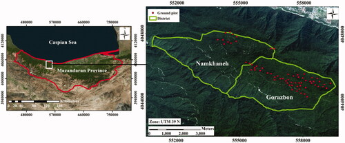
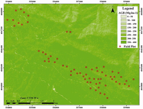
The study area is the Kheyruod research forest, which is located in the Hyrcanian forests, North of Iran. The Kheyruod forest research station was established in 1967 and is managed by the Department of Forest and Forest Economics, University of Tehran. It has an 8000-ha area and situated between Longitude 51°.32′–51°.43′ E, and Latitudes 36°.27–36°.40′ N. The kheyruod forest research consist of seven management districts. Figure 1 shows the distribution of the field plots over the Gorazbon and Namkhaneh districts. The elevation of the selected area ranges from 1000-m to 1500-m a.s.l. According to Nowshahr synoptic station, the mean annual precipitation is 1300-mm. The dominant species include Fagus Orientalis, Carpinus Betulus, Acer sp., and Alnus Subcordata.

Figure 1. Study area in Iran and the distribution of field plots (red dots) in the Gorazbon and Namkhaneh districts.

Field data

A nondestructive sampling method was conducted to estimate AGB in the field. Based on a typology map, we applied a stratified random sampling approach across the study area. We measured 65 field sample plots with an area of 2025-m² (45 m × 45 m) in beech dominant tree stands (i.e., stands with beech fraction more than 80%). Field sampling was performed in August 2014 (Figure 1). On each plot, tree species and diameter at breast height (DBH) were recorded. All trees with DBH larger than 7.5-cm were considered.

AGB estimation

The volume of each individual tree was calculated using a Tariff table. The Tariff table was developed for Gorazbon and Namkhaneh forest districts to predict tree volume based on DBH attribute by the Forestry and Forest Economics Department, University of Tehran. Tree biomass was calculated using equation (1)(1) $$\mathrm{A}GB=V\times \mathit{WCD}\mathrm{ }$$(1) (Enayati 2011; Brown and Lugo 1984). (1) $$\mathrm{A}GB=V\times \mathit{WCD}\mathrm{ }$$(1) where AGB is aboveground tree biomass (Mg.ha⁻¹), V is the volume of a tree derived from the Tariff table, and WCD is wood-critical density. The value of 0.56 Mg/m³ was used for Fagus Orientalis as wood critical density (Tarmian et al. 2009). Individual tree biomass was summed up to calculate plot-level AGB (Mg·ha⁻¹). The field data were split randomly into a training dataset (i.e., 70% of the field sample plots) and a validation dataset (i.e., 30% of the field sample plots). Plot level AGB for training and validation datasets are summarized in Table 1.

Table 1. Summarized plot level AGB statistics.

Data	Attributes
	Minimum (Mg·ha^−1)	Maximum (Mg·ha^−1)	Mean (Mg·ha^−1)	Standard deviation (Mg·ha^−1)
Train (n = 45)	192.49	467.43	293.9	61.09
Validation (n = 20)	204.81	432.44	296.42	63.7
All (N = 65)	192.5	467.43	294.67	61.4

Remote sensing data

Three remote sensing datasets, including L8, S2, and S1, were used for Hyrcanian forest AGB estimation (Table 2). The L8 data were downloaded from the United States Geological Survey (USGS) Earth Explorer data portal (https://earthexplorer.usgs.gov/). The sentinel data was obtained from the European Space Agency (ESA) Copernicus Open Access Hub (https://scihub.copernicus.eu/dhus/#/home). The Sentinel Application Platform (SNAP) (version. 6) (http://step.esa.int/main/toolboxes/snap/) and IDRISI Selva software packages were used for L8 and Sentinel data processing. The digital topographic maps provided by the National Cartographic Center (NCC) of Iran at 1/25,000 scale were used to check the geometric accuracy of images. The detailed information on optical and SAR data processing is presented in the following sections. The spatial resolution of all images was resampled to 5-m resolution using Nearest Neighbor interpolation.

Table 2. Satellite imagery acquisition dates and metrics derived from L8, S2, and S1.

Mission	Observation date	Product	Predictor variable	Relevant band/index/channel	Description/Resolution
Landsat 8- OLI	August 18, 2014	Multispectral image Level-1C	Multispectral Bands	b2 Blue (B)	450–515nm/30m
				b3 Green (G)	525–600nm/30m
				b4 Red (R)	630–680nm/30m
				b5 Near-infrared (NIR)	845–885nm/30m
				b6 Shortwave infrared 1 (SWIR1)	1560–1660nm/30m
				b7 Shortwave infrared 2 (SWIR2)	2100–2300nm/30m
				b8 Panchromatic	500–680nm/15m
			Vegetation indices	RVI	(b5/b4)
				NDVI	(b5-b4)/(b5 + b4)
			Greenness	Greenness	Greenness
			PCA	Com1-PCA (b1-b7)	First comp. of PCA for all bands
				Com1-PCA (b1-b4)	First comp. of PCA for bands of 1-4
				Com1-PCA (b5-b6)	First comp. of PCA for bands of 5-6
				Com1-PCA (b6-b7)	First comp. of PCA for bands of 6-7
			Fusion	Fus (b2)	Fusion of b2 with b8 bands
				Fus (b3)	Fusion of b3 with b8 bands
				Fus (b4)	Fusion of b4 with b8 bands
				Fus (b5)	Fusion of b5 with b8 bands
				Fus (b6)	Fusion of b6 with b8 bands
				Fus (b7)	Fusion of b7 with b8 bands
Sentinel-2A- MSI	August 26, 2016	Multispectral image Level-1C	Multispectral Bands	b2 Blue (B)	458–523nm/10m
				b3 Green (G)	543–578nm/10m
				b4 Red (R)	650–680nm/10m
				b5 Red-edge 1 (RE1)	698–713nm/20m
				b6 Red-edge 2 (RE2)	733–748nm/20m
				b7 Red-edge 3 (RE3)	773–793nm/20m
				b8 Near infrared (NIR)	785–900nm/10m
				b8a Near infrared narrow (NIRn)	855–875nm/20m
				b11 Shortwave infrared 1 (SWIR1)	1565–1655nm/20m
				b12 Shortwave infrared 2 (SWIR2)	2100–2280nm/20m
				LAI	Leaf Area Index
				Cab	Chlorophyll content in the leaf
				CWC	Canopy water content
				FAPAR	Fraction of absorbed photosynthetically active radiation
			Vegetation biophysical variables	FCOVER	Fraction of vegetation cover
			Vegetation indices	DVI	(b8-b4)
				GEMI	(n(1-0.25n)-(b3-0.125/1-b4))
				GNDVI	(b7-b3)/(b7 + b3)
				IPVI	(b8/(b8 + b4))
				IRECI	(b7-b4)/(b5/b6)
				MTCI	(b6-b5)/(b5-b4)
				NDI45	(b5-b4)/(b5 + b4)
				PSSRA	(b7/b4)
				REIP	700 + 40*((((b7 + b4)/2)-b5)/(b6-b5))
				RVI	(b8/b4)
				S2REP	705 + 35*((((b4–b7)/2)- b5)/(b6-b5))
				NDVI (b8 and b4)	(b8-b4)/(b8 + b4)
				NDVI (b8a and b4)	(b8a-b4)/(b8a + b4)
				NDVI-b6	(b4-b6)/(b4 + b6)
				NDVI-b8a	(b4-b8a)/(b4 + b8a)
			PCA	Com1-PCA (All Bands)	First comp. of PCA for all bands
				Com1-PCA (All Bands exception of b1, b9, b10)	First comp. of PCA for all bands exception of 1,9 and 10 bands
				Com1-PCA (b2–b8, b11, b12)	First comp. of PCA for bands of 2, 8, 11, and 12)
			Greenness	Greenness	Greenness
Sentinel-1A	August 22, 2015	S1A_IW_GRDH	Polarization/channel	VH	Vertical transmit-Horizontal channel (dB)
				VV	Vertical transmit-Vertical channel (dB)
				Ratiovhvv	Cross polarized ratio (VH/VV) (dB)
				Diffvhvv	Polarisations difference (VH-VV) (dB)
				Multvhvv	Polarisations multiply (VH*VV) (dB)
				Meanvhvv	Polarisations mean (VH + VV)/2 (dB)
				Square rootvhvv	Polarizations square root ($\sqrt{\mathit{\text{VH*VV}}}$) (dB)

Optical data processing

The radiometric quality of data was assessed. S2 Level-1C data were corrected to obtain a level-2A dataset using the SEN2COR atmospheric processor (http://step.esa.int/main/third-party-plugins-2/sen2cor/). In addition to the spectral bands, previous studies recommended using the transformed procedures to generate more spectral metrics sensitive to the forest structural attributes variation, i.e., vegetation indices, Tasseled Cap transformation (Greenness component) (Nedkov 2017; Ali Baig et al. 2014), Principle Component Analysis (PCA), Fusion of spectral bands with the panchromatic band (applied only to OLI data), and canopy biophysical and biochemical indices such as Leaf Area Index (LAI), Leaf Chlorophyll Content (Cab), Canopy Water Content (CWC) and Fraction of Absorbed Photosynthetically Active Radiation (FAPAR) (applied to MSI data) (Table 2). These mentioned biophysical indices are computed using PROSAIL radiative transfer model (For detailed information, please refer to Weiss and Baret 2016; Jacquemoud et al. 2009). Many studies have shown the efficiency of these transformed spectral metrics for vegetation attributes estimation (Liu et al. 2019; Putzenlechner et al. 2019; Chen et al. 2018; Castillo et al. 2017; Frampton et al. 2013).

SAR data processing

The Ground Range Detection (GRD) images were radiometrically calibrated and the values were converted to the Ƴ° backscatter coefficient according to the local incidence angle (Poorazimy et al. 2017; Tsui et al. 2012; Kellndorfer et al. 1998). The Refined Lee filter was applied to reduce the speckle effect. The terrain correction procedure was implemented on all images and finally inverted to dB using equation (2)(2) $$DN\left(dB\right)=10\hspace{0.17em}\text{log}\hspace{0.17em}10\left(N\right)\mathrm{ }$$(2) . (2) $$DN\left(dB\right)=10\hspace{0.17em}\text{log}\hspace{0.17em}10\left(N\right)\mathrm{ }$$(2) where N is the value extracted from the preprocessed SAR images. Many studies have shown a direct relationship between polarization channels and vegetation AGB (Liu et al. 2019; Chen et al. 2018; Castillo et al. 2017). Therefore, we also used $\frac{VH}{VV}, VH-VV, VH\times VV, \frac{VH+VV}{2}\mathit{\text{and }}\sqrt{VH}\times VV$ as predictor variables (Table 2).

Correlation analysis and AGB modeling

We used the Pearson correlation analysis to determine the strength of relationships between AGB and remote sensing derived metrics. To predict forest AGB (dependent variable) from remote sensing metrics (independent variables), parametric and non-parametric approaches were applied. We used the stepwise multiple linear regression (MLR) model as the most common parametric approach (Poorazimy et al. 2020; Lu et al. 2016; Kumar et al. 2013). In addition, different non-parametric approaches, i.e., k-NN (Tomppo 1990; Tomppo and Halme 2004), RF (Breiman 2001), and SVR (Cortes and Vapnik 1995; Vapnik 1995) were also assessed. Before implementing the MLR, the normality assumption of the dataset was checked using the Kolmogorov–Smirnov Test (Tojal et al. 2019; Kleinbaum et al. 2013). The collinearity was assessed using the Variance Inflation Factor (VIF) and Tolerance Index to ensure that the predictors were not highly correlated (Tojal et al. 2019; Kleinbaum et al. 2013). We also used the Durbin-Watson statistic to investigate the residual’s autocorrelation (Tojal et al. 2019; Kleinbaum et al. 2013). It is important to mention that only statistically significant predictors obtained from the Pearson correlation analysis were used in AGB modeling.

We used four different distance metrics, i.e., Euclidean, Euclidean Squared, Mahalanobis, and Manhattan, for determining the best number of k nearest neighbors with the k-NN method. In the case of the RF algorithm, the optimal k predictors were calculated as a square root of the predictor variables number ±2. Also, the optimal number of decision trees was determined based on the average squared errors of training and validation datasets. We considered four different kernels for the SVR algorithm, including Linear, Polynomial, Radial Basis Function (RBF), and Sigmoid. The statistical analysis was implemented using Statistica (version 10) and SPSS (version 22) software.

Accuracy assessment

The Coefficient of determination (R²), Root Mean Square Error (RMSE), relative RMSE (rRMSE), and Akaike Information Criterion (AIC) were used as criteria metrics for selecting the best fitting models for the validation dataset (Equations 3–6). (3) $${\mathrm{r}}^2=\frac{{\left[{\sum }_{i=1}^N(O_i-\overline{O})(P_i-\overline{P})\right]}^2}{\left(\sqrt{{\sum }_{i=1}^N(O_i-\overline{O}})\right)\left(\sqrt{{\sum }_{i=1}^N(P_i-\overline{P})}\right)}$$(3) (4) $$\mathit{RMSE}={\left[N^{-1}\sum _{i=1}^N{(P_i-O_i)}^2\right]}^{-0.5}\mathrm{ }$$(4) (5) $$\mathit{rRMSE}=\frac{\mathit{RMSE}}{\overline{O}}\times 100$$(5) (6) $$\mathit{AIC}=\mathit{Nln}\left(\mathit{RMSE}\right)+2t$$(6) where N is the number of field data, O_i is the observed value, P_i is the predicted value, $\overline{O}$ 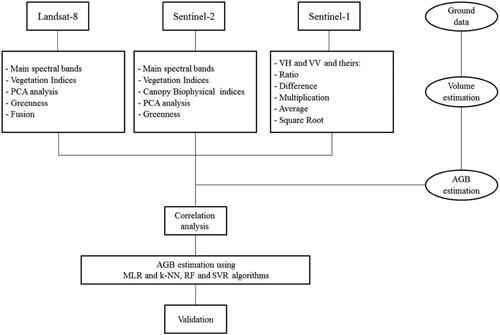is the average of observed values, and t is the number of predictors in the model. The flowchart of the methodology is presented in Figure 2.

Figure 2. The flowchart of applied methodology to predict forest AGB.

Results

Correlation analysis

The applied normality test showed that the data are normally distributed (p = 0.85). The Pearson correlation coefficients computed for AGB and remote sensing derived metrics are provided in Table 3. The most important metrics to estimate forest AGB were the first component of Principle Component Analysis (PCA) using the spectral bands for L8 (r = 0.367), FAPAR for S2 (r = 0.42), and VH Ƴ° backscatter coefficient (r=-0.351) for S1. It can be seen from Table 3 that S2 metrics showed the highest correlation for AGB estimates, and as we will explain in the next section, S2 was the best dataset in both individual and combination forms.

Table 3. Correlation analysis between AGB and remote sensing derived metrics.

Satellite	Variable	Correlation coefficient Sig. (r)	Satellite	Variable	Correlation coefficient Sig. (r)
Landsat-8	b2	0.001 ^ns	Sentinel-2	Cab	0.388**
	b3	0.276*		CWC	0.231 ^ns
	b4	0.197 ^ns		FAPAR	0.42**
	b5	0.361**		FCOVER	0.403**
	b6	0.349**		DVI	0.388**
	b7	0.298*		GEMI	0.395**
	b8	0.183 ^ns		GNDVI	0.366**
	VI	0.328**		IPVI	0.336**
	NDVI	0.34**		IRECI	0.374**
	Greenness	0.345**		MTCI	0.217 ^ns
	Com1-PCA(b1-b7)	0.367**		NDI45	0.067 ^ns
	Com1-PCA(b1-b4)	0.125 ^ns		PSSRA	0.294*
	Com1-PCA(b5-b6)	0.365**		REIP	0.259*
	Com1-PCA(b6-b7)	0.342**		RVI	0.322**
	Fus (b2)	−0.087 ^ns		S2REP	0.259*
	Fus (b3)	0.021 ^ns		NDVI (b8 and b4)	0.336**
	Fus (b4)	−0.018 ^ns		NDVI (b8a and b4)	0.328**
	Fus (b5)	0.329*		Com1-PCA (All Bands)	0.38**
	Fus (b6)	0.148 ^ns		Com1-PCA (All Bands except b1, b9, b10)	0.381**
	Fus (b7)	0.055 ^ns		Com1-PCA (b2-b8, b11, b12)	0.38**
Sentinel-2	b2	0.156 ^ns		NDVI-b6	0.38**
	b3	0.22 ^ns		NDVI-b8a	0.417**
	b4	0.283*		Greenness	0.394**
	b5	0.194 ^ns	Sentinel-1	VH	−0.351**
	b6	0.334**		VV	−0.295*
	b7	0.382**		Ratvhvv	−0.157 ^ns
	b8	0.395**		Diffvhvv	0.009 ^ns
	b8a	0.395**		Multvhvv	0.341**
	b11	0.275*		Meanvhvv	−0.345**
	b12	0.182 ^ns		Square rootvhvv	−0.336**
	LAI	0.384**

ns: non-significant correlation; *significant at 95% confidence interval; **significant at 99% confidence interval.

AGB modeling using MLR algorithm

The best models obtained from remotely sensed derived metrics and stepwise MLR are shown in Table 4. A combination of S2 and S1 datasets, i.e., FAPAR canopy biophysical index and VH Ƴ° backscatter coefficient as predictors, explained more variability in forest AGB (R²=0.34 and rRMSE = 17%). Figure 3 shows that the residual graph is normally distributed. A combination of L8 and S1, and S2 datasets were in the second and third order of accuracy with rRMSE 53.33 and 54.54%, respectively.

Figure 3. Histogram and normal P–P plot of residuals for normality assessment.

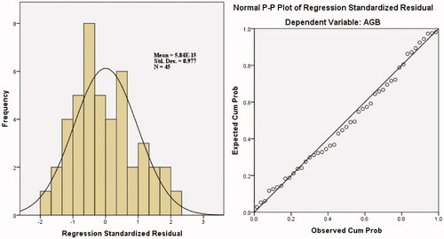
Table 4. Selected models to estimate forest AGB based on stepwise MLR algorithm and multi-sensor datasets.

Dataset	Model	Durbin–Watson statistic	VIF statistic	Tolerance statistic	RMSE (Mg.ha^−1)	rRMSE (%)	R^2	AIC
Landsat-8	AGB = 0.152 b7-924.819	1.578	1	1	64.77	21.85	0.009	85.4
	(AdjR^2=0.137)
Sentinel-2	AGB = 903.607 FAPAR − 288.152	1.715	1	1	54.54	18.4	0.28	81.9
	(AdjR^2=0.126)
Sentinel-1	AGB=-15.802VH + 52.138	1.556	1	1	56.83	19.17	0.17	82.8
	(AdjR^2=0.082)
Landsat-8 and Sentinel-1	AGB = 0.052 Com1-PCA (b6–b7)	1.747	1	1	53.33	17.99	0.28	81.5
	−14.434 VH − 681.647
	(AdjR^2=0.199)
Sentinel-2 and Sentinel-1	AGB = 926.213 FAPAR-16.356VH − 552.956	1.998	1	1	50.4	17	0.34	80.4
	(AdjR^2=0.221)

AGB modeling using non-parametric approaches

The results of k-NN for five sources of remote sensing datasets are summarized in Table 5. S2 dataset with rRMSE 16.99% showed higher potential for AGB estimation than S1 dataset with rRMSE 19.37%. The incorporation of S2 and S1 datasets performed better than other datasets. Among distance metrics, Manhattan produced more accurate results (i.e., R² of 0.57 and an rRMSE of 14.68%).

Table 5. The results of the k-NN algorithm for AGB estimation using multi-sources remote sensing datasets.

Dataset	Metrics	RMSE(Mg.ha^−1)	rRMSE (%)	(R^2)	(AIC)
Landsat-8	Euclidean	58.84	19.85	0.109	83.5
	Euclidean Squared	59.46	20.06	0.083	83.7
	Chebychev	59.24	19.98	0.104	83.6
	Manhatan	56.18	18.95	0.184	82.5
Sentinel-2	Euclidean	54.84	18.5	0.356	82
	Euclidean Squared	53.29	17.98	0.353	81.5
	Chebychev	56.93	19.21	0.287	82.8
	Manhatan	50.37	16.99	0.361	80.3
Sentinel-1	Euclidean	57.78	19.49	0.184	83.1
	Euclidean Squared	57.75	19.48	0.182	83.1
	Chebychev	57.42	19.37	0.192	83
	Manhatan	57.84	19.51	0.184	83.1
Landsat-8 and Sentinel-1	Euclidean	55.64	18.77	0.312	82.4
	Euclidean Squared	55.73	18.81	0.274	82.4
	Chebychev	60.41	20.38	0.06	84
	Manhatan	54.14	18.26	0.258	81.8
Sentinel-2 and Sentinel-1	Euclidean	52.46	17.5	0.468	81.2
	Euclidean Squared	48.93	16.5	0.51	79.8
	Chebychev	57.66	19.45	0.221	83.1
	Manhatan	43.5	14.68	0.57	77.5

The RF algorithm gained better results again for a combination of the S2 and S1 datasets (Table 6). The final RF model consists of 8 predictors with 500 trees that showed the highest predictive accuracy (R²=0.5 and rRMSE = 18.6%). Unlike our expectations, the S1 dataset had lower performance in comparison with other datasets for AGB estimation with R²=0.126 and rRMSE 20.02%.

Table 6. RF algorithm performance to estimate AGB using multi-sources remote sensing datasets.

Dataset	Optimal number of trees	Number of predictor (k)	RMSE(Mg.ha^⊟1)	rRMSE (%)	(R^2)	(AIC)
Landsat-8	500	3	58.8	19.86	0.139	83.5
	500	4	58.7	19.8	0.135	83.4
	500	5	58.03	19.57	0.159	83.2
	500	6	58.03	19.58	0.186	83.2
	500	7	59.73	20.15	0.083	83.7
Sentinel-2	450	4	56.72	19.13	0.406	82.76
	450	5	56.95	19.21	0.424	82.8
	450	6	56.06	18.91	0.46	82.5
	450	7	56.42	19.03	0.418	82.6
	450	8	56.44	19.03	0.417	82.6
Sentinel-1	250	1	59.38	20.03	0.146	83.6
	250	2	59.35	20.02	0.126	83.6
	250	3	59.41	20.04	0.117	83.6
	250	4	59.54	20.08	0.109	83.7
	250	5	59.6	20.1	0.115	83.7
Landsat-8 and Sentinel-1	500	3	56.84	19.17	0.349	82.8
	500	4	57.47	19.39	0.23	83
	500	5	57.36	19.35	0.27	82.9
	500	6	56.97	19.22	0.3	82.8
	500	7	57.28	19.32	0.253	82.9
Sentinel-2 and Sentinel-1	500	4	56.16	18.94	0.51	52.5
	500	5	55.94	18.87	0.54	82.4
	500	6	56.31	19	0.51	82.6
	500	7	55.74	18.8	0.47	82.4
	500	8	55.12	18.6	0.5	89.19

The SVR models showed that a combination of S2 and S1 datasets had better performance than other datasets (Table 7). The selected SVR model with a sigmoid kernel explained 17.307% of forest AGB variation. The low R²=0.052 for L8 showed no meaningful relationship for AGB estimates, while the S2 dataset had a second order of accuracy with rRMSE 17.93% among other datasets.

Table 7. SVR algorithm performance to estimate AGB using multi-sources remote sensing datasets.

Dataset	Kernel	RMSE(Mg.ha^−1)	rRMSE (%)	(R^2)	(AIC)
Landsat-8	Linear	72.05	24.03	0.0002	81.3
	Polynomial	64.59	21.79	0.052	85.3
	Radial basis Function kernel (RBF)	65.89	22.23	0.0001	85.7
	Sigmoid	74.59	25.16	0.00001	88.2
Sentinel-2	Linear	59.43	20.05	0.17	83.7
	Polynomial	57.45	19.38	0.34	83
	Radial basis function kernel (RBF)	53.15	17.93	0.31	81.4
	Sigmoid	89.51	30.2	0.025	91.8
Sentinel-1	Linear	–	–	–	–
	Polynomial	60.26	20.33	0.061	83.9
	Radial basis function kernel (RBF)	58.34	19.64	0.128	83.3
	Sigmoid	59.2	19.97	0.106	83.6
Landsat-8 and Sentinel-1	Linear	62.02	20.93	0.063	84.5
	Polynomial	59.52	20.08	0.095	83.7
	Radial basis function kernel (RBF)	56.14	18.94	0.228	82.5
	Sigmoid	55.96	18.88	0.249	82.5
Sentinel-2 and Sentinel-1	Linear	52.22	17.62	0.306	81.1
	Polynomial	54.37	18.342	0.348	81.9
	Radial basis function kernel (RBF)	53.41	18.02	0.27	81.5
	Sigmoid	51.3	17.307	0.368	80.7

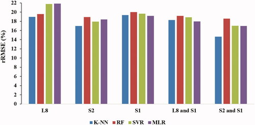
In general, the integration of the S2 and S1 datasets with the k-NN algorithm produced the best results for AGB estimation in our study area. As expected, S2 was more complementary with S1 rather than L8. The scatter plot of predicted versus measured AGB using the best combination dataset has been reported in Figure 4. As it is observed, the fitted model had more ability to predict AGB until 200 trees/ha. The generated AGB map using the best model has shown in Figure 5.

Figure 4. The estimated versus measured AGB based on S2 and S1 dataset (k-NN algorithm).

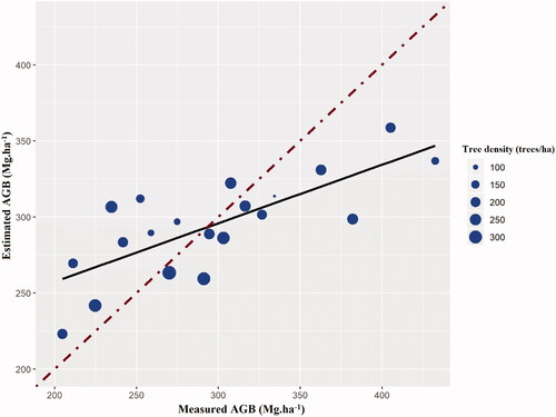
Figure 5. Predicted AGB over the study area using S2 and S1 dataset and k-NN algorithm.

Discussion

The relationships between AGB and remote sensing derived metrics

L8 dataset showed that the first component of PCA applied to spectral bands (b1–b7) is most relevant to forest AGB estimation than other L8 variables with r = 0.367. Then, the first PCA component using bands 5-6, band-5 (NIR), band-6 (SWIR1), and Greenness component were highly correlated with AGB, respectively. Data fusion between band-5 (NIR) and panchromatic band significantly improved AGB estimation, but other fused bands did not show a high correlation. For the S2 dataset, the highest correlation observed for FAPAR biophysical index (r = 0.42), following by NDVI (based on the red-edge spectral band (NIR-b8a) and FCOVER canopy biophysical index with the correlation of 0.417 and 0.403, respectively. In several studies, the efficiency of canopy biophysical indices derived from the S2 dataset to predict vegetation attributes has been proved (Liu et al. 2019; Chen et al. 2018; Castillo et al. 2017). Also, we found that S2 spectral bands are positively correlated with AGB. Among them, a high correlation was obtained for band-8 (785–900-nm) and Band-8a (855–875-nm) with a correlation of 0.395. Three red-edge spectral bands acquired by S2 seem promising data to estimate vegetation properties. The first red-edge band (b5) did not show any significant correlation with AGB. This is in accordance with Korhonen et al. (2017) for LAI estimation and in contrast to Chrysafis et al. (2017) for AGB estimation. Red band (b4, r =0.283) and second and third red-edge bands (b6, r = 0.334 and b7, r = 0.382) had positive correlation with AGB. According to obtained results, there is a need for more investigation about this phenomenon. The sensitivity of vegetation indices to AGB changes was observed in our study (Table 3), which is in line with the results of other studies (Liu et al. 2019; Pham and Brabyn 2017; Sousa et al. 2015; Zhu and Liu 2015). Also, Vafaei et al. (2017) reported a lower RMSE for AGB estimation using vegetation indices than ALOS-2 data in the Hyrcanian forest.

Most of the metrics derived from optical remotely sensed datasets showed significantly correlation with forest AGB in these broadleaved temperature forests. This means that with increasing forest AGB value, the reflectance is also increased. Because of the high canopy density and multi-storied Fagetum community in our study area, there was not any reflectance from the ground and floor vegetation. So, this can be a reason for our significant results. Our results were in the range of some other studies (Yadav and Nandy 2015; Amini Baneh 2013; Lu 2005).

The correlation analysis for the S1 dataset also showed a significant negative correlation between AGB and VH and VV Ƴ° backscatter coefficients (i.e., with the correlation of −0.351 and −0.295, respectively). Such significant relationships between the polarimetric channels (i.e., VH and VV) and AGB have been reported in other studies (Kumar et al. 2019; Omar et al. 2017; Suzuki et al. 2013). Van Pham et al. (2019) showed that metrics computed by mathematical operation on different polarization channels were important for AGB estimation. We also found that multiplication, average, and root of multiplied polarimetric channels with the correlation of 0.341, −0.345, and −0.336, respectively produced more relevant metrics than VV Ƴ° backscatter coefficient for AGB estimation. In contrast, we did not observe any significant relationships between forest AGB and two metrics of ratio and difference between two polarimetric channels.

The performance of MLR and non-parametric approaches for AGB estimation

The best MLR model with rRMSE = 17% was based on a combination of S2 and S1 datasets, in which the FAPAR canopy biophysical index and VH Ƴ° backscatter coefficient were selected as predictors. In terms of accuracy for AGB estimation, the second and third models were a combination of L8 and S1, and S2 datasets, respectively. For L8 and S1 combination, the first component of PCA transformation applied to bands of 5–6 and VH Ƴ° backscatter coefficient were selected as predictors and yielded an rRMSE of 18%. For the S2 dataset, the metric of FAPAR was the most effective variable for AGB estimation and achieved an rRMSE of 18.4%. Parametric models might fail to provide good performance for estimating forest structural attributes because of their restricted assumptions. In practice, the relationships between AGB and remote sensing metrics are very complex, which resulted in low accuracy for parametric models. In contrast, non-parametric approaches have a predefined simple data structure and, with their flexibility, showed more potential for AGB estimation (Lu et al. 2016). We found a better performance for non-parametric approaches compared to the parametric MLR approach. Our results showed that the k-NN algorithm using a combination of S2 and S1 datasets produced the most accurate results than the other datasets and algorithms. The observed R² and rRMSE were 0.57 and 14.68%, respectively. Our results showed that the k-NN method improved the AGB rRMSE relative to SVR, RF, and MLR by 2.62, 3.92, and 2.32%. Chirici et al. (2016) summarized the results of 148 studies from 26 different countries in which forest structure attributes have been estimated using remote sensing datasets. They showed that the k-NN algorithm was a reliable approach for predicting forest structural attributes at different scales (i.e., local to global). Our k-NN related results are in accordance with findings of previous studies (Persson et al. 2021; Poorazimy et al. 2020; Mura et al. 2018; Bilous et al. 2017; Chirici et al. 2016; McRoberts et al. 2015; Yadav and Nandy 2015; Beaudoin et al. 2014; Gagliasso et al. 2014; Jung et al. 2013; Tian et al. 2014; Tomppo et al. 2008; McRoberts et al. 2007; Maselli et al. 2005; Tomppo and Halme 2004). Application of RF algorithm for AGB estimation had a better result for the combination of S2 and S1 dataset with R² = 0.5 while it was worst for S1 dataset. However, there are many successful reports that show the performance of the RF algorithm for AGB estimation within different biophysical conditions (Liu et al. 2019; Ghosh and Behera 2018; Pandit et al. 2018; Chrysafis et al. 2017; Pflugmacher et al. 2014; Tanase et al. 2014; Latifi et al. 2010). Also, we found an rRMSE of 17.93% for AGB estimation using the S2 dataset and SVR algorithms. Similar results have been reported by Navarro et al. (2019), Chen et al. (2018), López-Serrano et al. (2016), Mountrakis et al. (2011), and Camps-Valls (2009). One of the advantages of the SVR algorithm is its capacity to deal with a low number of field sample plots (Lu et al. 2016). Also, SVR can predict the non-linear relationships between dependent and independent variables. Vafaei et al. (2017) have reported an R² of 0.61 for AGB estimation using the SVR algorithm in a small part of the Hyrcanian forest. They used the S2 dataset, and their reported accuracy is similar to our results. The performance of different approaches and datasets for AGB modeling is shown in Figure 6. It demonstrates that the k-NN algorithm is well suited for forest AGB prediction compared to other algorithms. The lowest rRMSE was obtained using a combination of S2 and S1 datasets. Our results provide supporting evidence that a combination of active and passive datasets offers the optimal capability and sensitivity to model structural attributes, particularly over complex forest ecosystems (Fatehi et al. 2015). It is worth mentioning that there was a two-year time lag between S2 data and field sample plot collection while the S2 dataset showed its notable performance. In addition, significant revisit time of the S2 dataset may have a great potential for monitoring structural developments. As Mura et al. (2018) reported a better performance for S2 compared to the Landsat-8 and RapidEye. Chrysafis et al. (2017) and Astola et al. (2019) also confirmed that S2 was more successful than L8 for predicting structural attributes.

Figure 6. The performance of each dataset with different modeling algorithm for AGB estimation.

S1 dataset has been used more in the sparse forests with low biomass and pastures (Castillo et al. 2017; Sinha et al. 2015). In our study area, the forest has a complex structure and high density of biomass, which may negatively affect SAR data’s sensitivity. One of the reasons for weak results obtained from SAR data is the saturation of the C-band in high biomass levels. Our minimum value of AGB is close to 200 Mg.ha⁻¹. Although the non-parametric approaches performed better than MLR for the S1 dataset, the uncertainty is still high.

In our study, some uncertainties have been included in the AGB estimation procedure. First, the limited penetration into forest vertical structure caused some errors because most of the AGB concentration is in the trunk of trees (Lu et al. 2016). The temporal distance between remote sensing images and field data collection is the second influencing factor in our results. There was a two-year time lag between S2 data and field measurement sample plots. Third, we did not have access to the species-specific allometric equations for our study area. Therefore, there are uncertainties with using the general equation. Furthermore, the possible errors in the volume table could affect the results. Moreover, the GPS positional errors have a substantial impact on the results obtained from remote sensing studies. Finally, all metrics derived from spectral reflectance are affected by the atmosphere, soil moisture, phenology, and vegetation growth (Lu et al. 2016). All metrics place emphasis on the necessity of uncertainty analyses before formulating any final conclusion.

According to previous studies and our results, the L8, S2, and S1 datasets individually are not good enough for estimating forest AGB over the pure Fagus Orientalis at the plot level. The results support Moradi et al. (2018), which also stated that Landsat-8 datasets for AGB estimating in Carpinus Betulus stands in Hyrcanian forests have limitations. However, some studies have reported an acceptable performance of these datasets in the mixed forest stands (Amini Baneh 2013; Rostami Andargoli 2008). The results present the differences in the type of sensors, sampling method, size and number of field sample plots, tree species, and structure of forest stands play important roles in the comparison of results. Therefore, there is a need for more research over the temperate broad-leaved forests. In accordance with past literature, the integration of different remote sensing datasets can improve the precision of results (Zhang et al. 2019; Vafaei et al. 2017; Chang and Shoshany 2016; Sinha et al. 2016; Shen et al. 2016; Laurin et al. 2013) and this strategy is recommended for future studies in Hyrcanian mixed forests of Iran.

Conclusion

Forest ecosystems play a crucial role in mitigating and adapting to climate change as they are the largest terrestrial carbon sink. Conversely, climate change can drive forest ecosystem loss and therefore there is a need for accurate and timely forest ecosystems monitoring. In this study, we evaluated the capability of spectral and transformed bands of L8, S2, and S1 for AGB estimation. The limited ability of optical and short-wavelength SAR data to penetrate the vertical structure of forests resulted in low sensitivity for forest AGB estimation. In comparison, the combination of optical and SAR datasets improved the forest AGB estimation accuracy when they were used individually. In this regard, S2 was more complementary than L8 when used in combination with S1. Very likely, it is because of a higher spatial resolution of S2 and the presence of red-edge bands and derived canopy biophysical indices. By combining remotely sensed datasets, the selected algorithm should be able to accommodate the different characteristics of multi-source data for AGB estimation. In addition, the relationship between AGB and remote sensing-based metrics is often complex, so comparative analyses to select the most accurate prediction technique is a common and necessary approach. We found that the k-NN algorithm has better performance than MLR, RF, and SVR algorithms. It is worth mentioning that each of the prediction algorithms has its own region of best performance, and the results are specific to each study area. Still, any generalization should be performed with caution and not without local validation. The use of LiDAR data and long-wavelength SAR data is recommended for future studies because they penetrate the vertical structure of the forest, which includes the most relevant component for AGB estimation. Also, providing species-specific allometric equations for AGB estimating is essential to predict accurate forest AGB.

Disclosure statement

No potential conflict of interest was reported by the author(s).

References

- Ali Baig, M.H.A., Zhang, L., Shuai, T., and Tong, Q. 2014. “Derivation of a tasselled cap transformation based on Landsat 8 at-satellite reflectance.” Remote Sensing Letters, Vol. 5(No. 5): pp. 423–431. doi:https://doi.org/10.1080/2150704X.2014.915434.
- Amini Baneh, S. 2013. Investigation on the possibility to estimation of forest above ground biomass using SPOT HRG sensor data and different algorithm of weighted K-Nearest Neighbor approach. M.Sc. Thesis. Iran: Sari Agriculture and Natural Resource University.
- Astola, H., Häme, T., Sirro, L., Molinier, M., and Kilpi, J. 2019. “Comparison of Sentinel-2 and Landsat 8 imagery for forest variable prediction in boreal region.” Remote Sensing of Environment, Vol. 223: pp. 257–273. doi:https://doi.org/10.1016/j.rse.2019.01.019.
- Beaudoin, A., Bernier, P.Y., Guindon, L., Villemaire, P., Guo, X.J., Stinson, G., Bergeron, T., Magnussen, S., and Hall, R.J. 2014. “Mapping attributes of Canada’s forests at moderate resolution through kNN and MODIS imagery.” Canadian Journal of Forest Research, Vol. 44(No. 5): pp. 521–532. doi:https://doi.org/10.1139/cjfr-2013-0401.
- Berninger, A., Lohberger, S., Stängel, M., and Siegert, F. 2018. “SAR-based estimation of above-ground biomass and its changes in tropical forests of Kalimantan using L-and C-Band.” Remote Sensing, Vol. 10(No. 6): pp. 831. doi:https://doi.org/10.3390/rs10060831.
- Bilous, A., Myroniuk, V., Holiaka, D., Bilous, S., See, L., and Schepaschenko, D. 2017. “Mapping growing stock volume and forest live biomass: a case study of the Polissya region of Ukraine.” Environmental Research Letters, Vol. 12(No. 10): pp. 105001. doi:https://doi.org/10.1088/1748-9326/aa8352.
- Breiman, L. 2001. “Random forests.” Machine Learning, Vol. 45(No. 1):pp. 5–32. doi:https://doi.org/10.1023/A:1010933404324.
- Brown, S., and Lugo, A.E. 1984. “Biomass of tropical forests: A new estimate based on forest volumes.” Science, Vol. 223 (No. 4642): pp. 1290–1294. doi:https://doi.org/10.1126/science.223.4642.1290.
- Brown, S., Schroeder, P., and Birdsey, R. 1997. “Aboveground biomass distribution of US eastern hardwood forests and the use of large trees as an indicator of forest development.” Forest Ecology and Management, Vol. 96(No. 1–2): pp. 37–47. doi:https://doi.org/10.1016/S0378-1127(97)00044-3.
- Camps-Valls, G., Muñoz-Marí, J., Gómez-Chova, L., Richter, K., and Calpe-Maravilla, J. 2009. “Biophysical parameter estimation with a semisupervised support vector machine.” IEEE Geoscience and Remote Sensing Letters, Vol. 6(No. 2): pp. 248–252. doi:https://doi.org/10.1109/LGRS.2008.2009077.
- Castillo, J.A.A., Apan, A.A., Maraseni, T.N., and Salmo, S.G. 2017. “Estimation and mapping of above-ground biomass of mangrove forests and their replacement land uses in the Philippines using Sentinel imagery.” ISPRS Journal of Photogrammetry and Remote Sensing, Vol. 134: pp. 70–85. doi:https://doi.org/10.1016/j.isprsjprs.2017.10.016.
- Chang, J., and Shoshany, M. 2016. “Mediterranean shrublands biomass estimation using Sentinel-1 and Sentinel-2.” IEEE International Geoscience and Remote Sensing Symposium (IGARSS), Beijing, China, July 2016.
- Chen, L., Ren, C., Zhang, B., Wang, Z., and Xi, Y. 2018. “Estimation of forest above-ground biomass by geographically weighted regression and machine learning with sentinel imagery.” Forests, Vol. 9(No. 10): pp. 582. doi:https://doi.org/10.3390/f9100582.
- Chirici, G., Mura, M., McInerney, D., Py, N., Tomppo, E., Waser, L.T., Travaglini, D., and McRoberts, R.E. 2016. “A meta-analysis and review of the literature on the k-Nearest Neighbors technique for forestry applications that use remotely sensed data.” Remote Sensing of Environment, Vol. 176: pp. 282–294. doi:https://doi.org/10.1016/j.rse.2016.02.001.
- Chrysafis, I., Mallinis, G., Siachalou, S., and Patias, P. 2017. “Assessing the relationships between growing stock volume and Sentinel-2 imagery in a Mediterranean forest ecosystem.” Remote Sensing Letters, Vol. 8(No. 6): pp. 508–517. doi:https://doi.org/10.1080/2150704X.2017.1295479.
- Cortes, C., and Vapnik, V. 1995. “Support-vectornetworks.” Machine Learning, Vol. 20(No. 3): pp. 273–297. doi:https://doi.org/10.1007/BF00994018.
- Delegido, J., Verrelst, J., Alonso, L., and Moreno, J. 2011. “Evaluation of Sentinel-2 red-edge bands for empirical estimation of green LAI and chlorophyll content.” Sensors, Vol. 11(No. 7): pp. 7063–7081. doi:https://doi.org/10.3390/s110707063.
- Drusch, M., Del Bello, U., Carlier, S., Colin, O., Fernandez, V., Gascon, F., Hoersch, B., et al. 2012. “Sentinel-2: ESA's optical high-resolution mission for GMES operational services.” Remote Sensing of Environment, Vol. 120: pp. 25–36. doi:https://doi.org/10.1016/j.rse.2011.11.026.
- Enayati, A. A. 2011. Wood Physics. Tehran: University of Tehran Press.
- Fatehi, P., Damm, A., Schaepman, M., and Kneubühler, M. 2015. “Estimation of alpine forest structural variables from imaging spectrometer data.” Remote Sensing, Vol. 7(No. 12): pp. 16315–16338. doi:https://doi.org/10.3390/rs71215830.
- Fernández-Manso, A., Fernández-Manso, O., and Quintano, C. 2016. “SENTINEL-2A red-edge spectral indices suitability for discriminating burn severity.” International Journal of Applied Earth Observation and Geoinformation, Vol. 50: pp. 170–175. doi:https://doi.org/10.1016/j.jag.2016.03.005.
- Frampton, W.J., Dash, J., Watmough, G., and Milton, J.M. 2013. “Evaluating the capabilities of Sentinel-2 for quantitative estimation of biophysical variables in vegetation.” ISPRS Journal of Photogrammetry and Remote Sensing, Vol. 82: pp. 83–92. doi:https://doi.org/10.1016/j.isprsjprs.2013.04.007.
- Fuchs, H., Magdon, P., Kleinn, C., and Flessa, H. 2009. “Estimating aboveground carbon in a catchment of the Siberian forest tundra: Combining satellite imagery and field inventory.” Remote Sensing of Environment, Vol. 113(No. 3): pp. 518–531. doi:https://doi.org/10.1016/j.rse.2008.07.017.
- Gagliasso, D., Hummel, S., and Temesgen, H. 2014. “A comparison of selected parametric and non-parametric imputation methods for estimating forest biomass and basal area.” Open Journal of Forestry, Vol. 04(No. 01): pp. 42–48. doi:https://doi.org/10.4236/ojf.2014.41008.
- Ghosh, S.M., and Behera, M.D. 2018. “Aboveground biomass estimation using multi-sensor data synergy and machine learning algorithms in a dense tropical forest.” Applied Geography, Vol. 96: pp. 29–40. doi:https://doi.org/10.1016/j.apgeog.2018.05.011.
- Hall, R.J., Skakun, R.S., Arsenault, E.J., and Case, B.S. 2006. “Modeling forest stand structure attributes using Landsat ETM + data: Application to mapping of aboveground biomass and stand volume.” Forest Ecology and Management, Vol. 225(No. 1–3): pp. 378–390. doi:https://doi.org/10.1016/j.foreco.2006.01.014.
- Huang, X., Ziniti, B., Torbick, N., and Ducey, M. 2018. “Assessment of forest above ground biomass estimation using multi-temporal C-band sentinel-1 and polarimetric L-band PALSAR-2 Data.” Remote Sensing, Vol. 10(No. 9): pp. 1424. doi:https://doi.org/10.3390/rs10091424.
- Immitzer, M., Vuolo, F., and Atzberger, C. 2016. “First experience with sentinel-2 data for crop and tree species classifications in Central Europe.” Remote Sensing, Vol. 8(No. 3): pp. 166. doi:https://doi.org/10.3390/rs8030166.
- Jacquemoud, S., Verhoef, W., Baret, F., Bacour, C., Zarco-Tejada, P.J., Asner, G.P., François, C., and Ustin, S.L. 2009. “PROSPECT + SAIL models: A review of use for vegetation characterization.” Remote Sensing of Environment, Vol. 113: pp. S56–S66. doi:https://doi.org/10.1016/j.rse.2008.01.026.
- Jung, J., Kim, S., Hong, S., Kim, K., Kim, E., Im, J., and Heo, J. 2013. “Effects of national forest inventory plot location error on forest carbon stock estimation using k-nearest neighbor algorithm.” ISPRS Journal of Photogrammetry and Remote Sensing, Vol. 81: pp. 82–92. doi:https://doi.org/10.1016/j.isprsjprs.2013.04.008.
- Kellndorfer, J.M., Pierce, L.E., Dobson, M.C., and Ulaby, F.T. 1998. “Toward consistent regional-to-global-scale vegetation characterization using orbital SAR systems.” IEEE Transactions on Geoscience and Remote Sensing, Vol. 36(No. 5): pp. 1396–1411. doi:https://doi.org/10.1109/36.718844.
- Khorrami, R., Darvishsefat, A.A., and Namiranian, M. 2008. “Investigation on the capability of Landsat7 ETM + data for standing volume estimation of beech stands.” Journal of the Iranian Natural Resources, Vol. 60(No. 4): pp. 1281–1289.
- Kleinbaum, D., Kupper, L., Nizam, A., and Rosenberg, E. 2013. Applied Regression Analysis and Other Multivariable Methods: Boston: Cengage Learning.
- Korhonen, L., Packalen, P., and Rautiainen, M. 2017. “Comparison of Sentinel-2 and Landsat 8 in the estimation of boreal forest canopy cover and leaf area index.” Remote Sensing of Environment, Vol. 195: pp. 259–274. doi:https://doi.org/10.1016/j.rse.2017.03.021.
- Kumar, A., Kishore, B.S.P.C., Saikia, P., Deka, J., Bharali, S., Singha, L.B., Tripathi, O.P., and Khan, M.L. 2019. “Tree diversity assessment and above ground forests biomass estimation using SAR remote sensing: A case study of higher altitude vegetation of North-East Himalayas, India.” Physics and Chemistry of the Earth, Parts A/B/C, Vol. 111: pp. 53–64. doi:https://doi.org/10.1016/j.pce.2019.03.007.
- Kumar, L., and Mutanga, O. 2017. “Remote sensing of above-ground biomass.” Remote Sensing, Vol. 9(No. 9): pp. 935. doi:https://doi.org/10.3390/rs9090935.
- Kumar, P., Sharma, L.K., Pandey, P.C., Sinha, S., and Nathawat, M.S. 2013. “Geospatial strategy for tropical forest-wildlife reserve biomass estimation.” IEEE Journal of Selected Topics in Applied Earth Observations and Remote Sensing, Vol. 6(No. 2): pp. 917–923. doi:https://doi.org/10.1109/JSTARS.2012.2221123.
- Latifi, H., Nothdurft, A., and Koch, B. 2010. “Non-parametric prediction and mapping of standing timber volume and biomass in a temperate forest: Application of multiple optical/LiDAR-derived predictors.” Forestry, Vol. 83(No. 4): pp. 395–407. doi:https://doi.org/10.1093/forestry/cpq022.
- Laurin, G.V., Balling, J., Corona, P., Mattioli, W., Papale, D., Puletti, N., Rizzo, M., Truckenbrodt, J., and Urban, M. 2018. “Above-ground biomass prediction by Sentinel-1 multitemporal data in central Italy with integration of ALOS2 and Sentinel-2 data.” Journal of Applied Remote Sensing, Vol. 12(No. 01): pp. 1. doi:https://doi.org/10.1117/1.JRS.12.016008.
- Laurin, G.V., Liesenberg, V., Chen, Q., Guerriero, L., Del Frate, F., Bartolini, A., Coomes, D., Wilebore, B., Lindsell, J., and Valentini, R. 2013. “Optical and SAR sensor synergies for forest and land cover mapping in a tropical site in West Africa.” International Journal of Applied Earth Observation and Geoinformation, Vol. 21: pp. 7–16. doi:https://doi.org/10.1016/j.jag.2012.08.002.
- Liu, Y., Gong, W., Xing, Y., Hu, X., and Gong, J. 2019. “Estimation of the forest stand mean height and aboveground biomass in Northeast China using SAR Sentinel-1B, multispectral Sentinel-2A, and DEM imagery.” ISPRS Journal of Photogrammetry and Remote Sensing, Vol. 151: pp. 277–289. doi:https://doi.org/10.1016/j.isprsjprs.2019.03.016.
- López-Serrano, P.M., López-Sánchez, C.A., Álvarez-González, J.G., and García-Gutiérrez, J. 2016. “A comparison of machine learning techniques applied to landsat-5 TM spectral data for biomass estimation.” Canadian Journal of Remote Sensing, Vol. 42(No. 6): pp. 690–705. doi:https://doi.org/10.1080/07038992.2016.1217485.
- Lu, D. 2005. “Aboveground biomass estimation using Landsat TM data in the Brazilian Amazon.” International Journal of Remote Sensing, Vol. 26(No. 12): pp. 2509–2525. doi:https://doi.org/10.1080/01431160500142145.
- Lu, D., Chen, Q., Wang, G., Liu, L., Li, G., and Moran, E. 2016. “A survey of remote sensing-based aboveground biomass estimation methods in forest ecosystems.” International Journal of Digital Earth, Vol. 9(No. 1): pp. 63–105. doi:https://doi.org/10.1080/17538947.2014.990526.
- Marvi Mohadjer, M. R. 2007. Silviclture. Tehran: University of Tehran Press.
- Maselli, F., Chirici, G., Bottai, L., Corona, P., and Marchetti, M. 2005. “Estimation of Mediterranean forest attributes by the application of k‐NN procedures to multitemporal Landsat ETM + images.” International Journal of Remote Sensing, Vol. 26(No. 17): pp. 3781–3796. doi:https://doi.org/10.1080/01431160500166433.
- McNairn, H., and Shang, J. 2016. “A review of multitemporal synthetic aperture radar (SAR) for crop monitoring.” Multitemporal Remote Sensing, Vol. 20: pp. 317–340. doi:https://doi.org/10.1007/978-3-319-47037-5_15.
- McRoberts, R.E., Naesset, E., and Gobakken, T. 2015. “Optimizing the k-Nearest Neighbors technique for estimating forest aboveground biomass using airborne laser scanning data.” Remote Sensing of Environment, Vol. 163: pp. 13–22. doi:https://doi.org/10.1016/j.rse.2015.02.026.
- McRoberts, R.E., Tomppo, E.O., Finley, A.O., and Heikkinen, J. 2007. “Estimating areal means and variances of forest attributes using the k-nearest neighbors technique and satellite imagery.” Remote Sensing of Environment, Vol. 111(No. 4): pp. 466–480. doi:https://doi.org/10.1016/j.rse.2007.04.002.
- Moradi, F., Darvishsefat, A.A., Namiranian, M., and Ronoud, G. 2018. “Investigating the capability of Landsat 8 OLI data for estimation of aboveground woody biomass of common hornbeam (Carpinus betulus L.) stands in Khyroud Forest.” Iranian Journal of Forest and Poplar Research, Vol. 26(No. 3): pp. 406–420. doi:98.1000/1735-0883.1397.26.406.73.3.1602.1583.
- Motlagh, M.G., Kafaky, S.B., Mataji, A., and Akhavan, R. 2018. “Estimating and mapping forest biomass using regression models and Spot-6 images (case study: Hyrcanian forests of north of Iran).” Environmental Monitoring and Assessment, Vol. 190(No. 6): pp. 352. doi:https://doi.org/10.1007/s10661-018-6725-0.
- Mountrakis, G., Im, J., and Ogole, C. 2011. “Support vector machines in remote sensing: A review.” ISPRS Journal of Photogrammetry and Remote Sensing, Vol. 66(No. 3): pp. 247–259. doi:https://doi.org/10.1016/j.isprsjprs.2010.11.001.
- Mura, M., Bottalico, F., Giannetti, F., Bertani, R., Giannini, R., Mancini, M., Orlandini, S., Travaglini, D., and Chirici, G. 2018. “Exploiting the capabilities of the Sentinel-2 multi spectral instrument for predicting growing stock volume in forest ecosystems.” International Journal of Applied Earth Observation and Geoinformation, Vol. 66: pp. 126–134. doi:https://doi.org/10.1016/j.jag.2017.11.013.
- Navarro, J., Algeet, N., Fernández-Landa, A., Esteban, J., Rodríguez-Noriega, P., and Guillén-Climent, M. 2019. “Integration of uav, sentinel-1, and sentinel-2 data for mangrove plantation aboveground biomass monitoring in Senegal.” Remote Sensing, Vol. 11(No. 1): pp. 77. doi:https://doi.org/10.3390/rs11010077.
- Nedkov, R. 2017. “Orthogonal transformation of segmented images from the satellite Sentinel-2.” Comptes Rendus de L’Acadˊemie Bulgare Des Sciences, Vol. 70(No. 5): pp. 687–692.
- Olson, J. S., Watts, J., and Allison, L. J. 1983. Carbon in live vegetation of major world ecosystems. Oak Ridge: Oak Ridge National Laboratory.
- Omar, H., Misman, M., and Kassim, A. 2017. “Synergetic of PALSAR-2 and Sentinel-1A SAR polarimetry for retrieving aboveground biomass in dipterocarp forest of Malaysia.” Applied Sciences, Vol. 7(No. 7): pp. 675. doi:https://doi.org/10.3390/app7070675.
- Ouchi, K. 2013. “Recent trend and advance of synthetic aperture radar with selected topics.” Remote Sensing, Vol. 5(No. 2): pp. 716–807. doi:https://doi.org/10.3390/rs5020716.
- Pan, Y., Birdsey, R.A., Fang, J., Houghton, R., Kauppi, P.E., Kurz, W.A., Phillips, O.L., et al. 2011. “A large and persistent carbon sink in the world's forests.” Science, Vol. 333(No. 6045): pp. 988–993. doi:https://doi.org/10.1126/science.1201609.
- Pandey, P.C., Srivastava, P.K., Chetri, T., Choudhary, B.K., and Kumar, P. 2019. “Forest biomass estimation using remote sensing and field inventory: A case study of Tripura, India.” Environmental Monitoring and Assessment, Vol. 191(No. 9): pp. 593–515. doi:https://doi.org/10.1007/s10661-019-7730-7.
- Pandit, S., Tsuyuki, S., and Dube, T. 2018. “Estimating above-ground biomass in sub-tropical buffer zone community Forests, Nepal, using Sentinel 2 data.” Remote Sensing, Vol. 10(No. 4): pp. 601. doi:https://doi.org/10.3390/rs10040601.
- Periasamy, S. 2018. “Significance of dual polarimetric synthetic aperture radar in biomass retrieval: An attempt on Sentinel-1.” Remote Sensing of Environment, Vol. 217: pp. 537–549. doi:https://doi.org/10.1016/j.rse.2018.09.003.
- Persson, H.J., Jonzén, J., and Nilsson, M. 2021. “Combining TanDEM-X and Sentinel-2 for large-area species-wise prediction of forest biomass and volume.” International Journal of Applied Earth Observation and Geoinformation, Vol. 96: pp. 102275. doi:https://doi.org/10.1016/j.jag.2020.102275.
- Pflugmacher, D., Cohen, W.B., Kennedy, R.E., and Yang, Z. 2014. “Using Landsat-derived disturbance and recovery history and lidar to map forest biomass dynamics.” Remote Sensing of Environment, Vol. 151: pp. 124–137. doi:https://doi.org/10.1016/j.rse.2013.05.033.
- Pham, L.T., and Brabyn, L. 2017. “Monitoring mangrove biomass change in Vietnam using SPOT images and an object-based approach combined with machine learning algorithms.” ISPRS Journal of Photogrammetry and Remote Sensing, Vol. 128: pp. 86–97. doi:https://doi.org/10.1016/j.isprsjprs.2017.03.013.
- Poorazimy, M., Shataee, S., McRoberts, R.E., and Mohammadi, J. 2020. “Integrating airborne laser scanning data, space-borne radar data and digital aerial imagery to estimate aboveground carbon stock in Hyrcanian forests, Iran.” Remote Sensing of Environment, Vol. 240: pp. 111669. doi:https://doi.org/10.1016/j.rse.2020.111669.
- Poorazimy, M., Shataee, S., Attarchi, S., and Mohammadi, J. 2017. “Estimation of aboveground biomass using Alos-Palsar data in Hyrcanian forests (Case study: ShastKalateh, Gorgan).” Forest and Wood Products, Vol. 70(No. 3): pp. 479–488. doi:https://doi.org/10.22059/JFWP.2017.212542.766.
- Putzenlechner, B., Castro, S., Kiese, R., Ludwig, R., Marzahn, P., Sharp, I., and Sanchez-Azofeifa, A. 2019. “Validation of Sentinel-2 fAPAR products using ground observations across three forest ecosystems.” Remote Sensing of Environment, Vol. 232: pp. 111310. doi:https://doi.org/10.1016/j.rse.2019.111310.
- Ronoud, G., and Darvishsefat, A.A. 2018. “Estimating aboveground woody biomass of Fagus orientalis stands in Hyrcanian forest of Iran using Landsat 5 satellite data (Case study: Khyroud Forest).” Geographic Space, Vol. 17(No. 60): pp. 117–129.
- Rostami Andargoli, M. 2008. Estimation of aboveground woody biomass stand forests using SPOT5 satellite data. M.Sc. Thesis. Iran: University of Guilan.
- Sentinel-1_Team. 2013. Sentinel-1 User Handbook. Paris, France: European Space Agency.
- Sentinel-2_Team. 2015. Sentinel-2 User Handbook. Paris, France: European Space Agency.
- Shen, W., Li, M., Huang, C., and Wei, A. 2016. “Quantifying live aboveground biomass and forest disturbance of mountainous natural and plantation forests in Northern Guangdong, China, based on multi-temporal Landsat, PALSAR and field plot data.” Remote Sensing, Vol. 8(No. 7): pp. 595. doi:https://doi.org/10.3390/rs8070595.
- Sinha, S., Jeganathan, C., Sharma, L.K., and Nathawat, M.S. 2015. “A review of radar remote sensing for biomass estimation.” International Journal of Environmental Science and Technology, Vol. 12(No. 5): pp. 1779–1792. doi:https://doi.org/10.1007/s13762-015-0750-0.
- Sinha, S., Jeganathan, C., Sharma, L.K., Nathawat, M.S., Das, A.K., and Mohan, S. 2016. “Developing synergy regression models with space-borne ALOS PALSAR and Landsat TM sensors for retrieving tropical forest biomass.” Journal of Earth System Science, Vol. 125(No. 4): pp. 725–735. doi:https://doi.org/10.1007/s12040-016-0692-z.
- Sousa, A.M., Gonçalves, A.C., Mesquita, P., and da Silva, J.R.M. 2015. “Biomass estimation with high resolution satellite images: A case study of Quercus rotundifolia.” ISPRS Journal of Photogrammetry and Remote Sensing, Vol. 101: pp. 69–79. doi:https://doi.org/10.1016/j.isprsjprs.2014.12.004.
- Su, H., Shen, W., Wang, J., Ali, A., and Li, M. 2020. “Machine learning and geostatistical approaches for estimating aboveground biomass in Chinese subtropical forests.” Forest Ecosystems, Vol. 7(No. 1): pp. 1–20. doi:https://doi.org/10.1186/s40663-020-00276-7.
- Suzuki, R., Kim, Y., and Ishii, R. 2013. “Sensitivity of the backscatter intensity of ALOS/PALSAR to the above-ground biomass and other biophysical parameters of boreal forest in Alaska.” Polar Science, Vol. 7(No. 2): pp. 100–112. doi:https://doi.org/10.1016/j.polar.2013.03.001.
- Tanase, M.A., Panciera, R., Lowell, K., Tian, S., Hacker, J.M., and Walker, J.P. 2014. “Airborne multi-temporal L-band polarimetric SAR data for biomass estimation in semi-arid forests.” Remote Sensing of Environment, Vol. 145: pp. 93–104. doi:https://doi.org/10.1016/j.rse.2014.01.024.
- Tarmian, A., Remond, R., Faezipour, M., Karimi, A., and Perré, P. 2009. “Reaction wood drying kinetics: Tension wood in Fagus sylvatica and compression wood in Picea abies.” Wood Science and Technology, Vol. 43(No. 1–2): pp. 113–130. doi:https://doi.org/10.1007/s00226-008-0230-5.
- Tian, X., Li, Z., Su, Z., Chen, E., van der Tol, C., Li, X., Guo, Y., Li, L., and Ling, F. 2014. “Estimating montane forest above-ground biomass in the upper reaches of the Heihe River Basin using Landsat-TM data.” International Journal of Remote Sensing, Vol. 35(No. 21): pp. 7339–7362. doi:https://doi.org/10.1080/01431161.2014.967888.
- Tojal, L.T., Bastarrika, A., Barrett, B., Sanchez Espeso, J.M., Lopez-Guede, J.M., and Graña, M. 2019. “Prediction of aboveground biomass from low-density LiDAR data: Validation over P. radiata data from a region north of Spain.” Forests, Vol. 10(No. 9): pp. 819. doi:https://doi.org/10.3390/f10090819.
- Tomppo, E. 1990. “Designing a satellite image-aided national forest survey in Finland. The usability of remote sensing for forest inventory and planning.” Proceedings from SNS/IUFRO workshop in Umeå, Umeå, Sweden, February 1990.
- Tomppo, E., and Halme, M. 2004. “Using coarse scale forest variables as ancillary information and weighting of variables in k-NN estimation: A genetic algorithm approach.” Remote Sensing of Environment, Vol. 92(No. 1): pp. 1–20. doi:https://doi.org/10.1016/j.rse.2004.04.003.
- Tomppo, E., Olsson, H., Ståhl, G., Nilsson, M., Hagner, O., and Katila, M. 2008. “Combining national forest inventory field plots and remote sensing data for forest databases.” Remote Sensing of Environment, Vol. 112(No. 5): pp. 1982–1999. doi:https://doi.org/10.1016/j.rse.2007.03.032.
- Tsui, O.W., Coops, N.C., Wulder, M.A., Marshall, P.L., and McCardle, A. 2012. “Using multi-frequency radar and discrete-return LiDAR measurements to estimate above-ground biomass and biomass components in a coastal temperate forest.” ISPRS Journal of Photogrammetry and Remote Sensing, Vol. 69: pp. 121–133. doi:https://doi.org/10.1016/j.isprsjprs.2012.02.009.
- Vafaei, S., Soosani, J., Adeli, K., Fadaei, H., and Naghavi, H. 2017. “Estimation of aboveground biomass using optical and radar images (case study: Nav-e Asalem forests, Gilan).” Iranian Journal of Forest and Poplar Research, Vol. 25(No. 2): pp. 320–331. doi:https://doi.org/10.22092/IJFPR.2017.111776.
- Van Pham, M., Pham, T.M., Du, Q.V.V., Bui, Q.T., Van Tran, A., Pham, H.M., and Nguyen, T.N. 2019. “Integrating Sentinel-1A SAR data and GIS to estimate aboveground biomass and carbon accumulation for tropical forest types in Thuan Chau district, Vietnam.” Remote Sensing Applications: Society and Environment, Vol. 14: pp. 148–157. doi:https://doi.org/10.1016/j.rsase.2019.03.003.
- Vapnik, V. N. 1995. The nature of statistical learning theory. New York: Springer-Verlag New York, Inc.
- Wani, A.A., Joshi, P.K., and Singh, O. 2015. “Estimating biomass and carbon mitigation of temperate coniferous forests using spectral modeling and field inventory data.” Ecological Informatics, Vol. 25: pp. 63–70. doi:https://doi.org/10.1016/j.ecoinf.2014.12.003.
- Weiss, M., and Baret, F. 2016. S2ToolBox Level 2 products: LAI, FAPAR, FCOVER, Version 1.1. In ESA Contract nr 4000110612/14/I-BG (p. 52); Paris, France: INRA Avignon.
- Wijaya, A., Kusnadi, S., Gloaguen, R., and Heilmeier, H. 2010. “Improved strategy for estimating stem volume and forest biomass using moderate resolution remote sensing data and GIS.” Journal of Forestry Research, Vol. 21(No. 1): pp. 1–12. doi:https://doi.org/10.1007/s11676-010-0001-7.
- Wu, C.F., Shen, H.H., Shen, A.H., Deng, J.S., Gan, M.Y., Zhu, J.X., Xu, H.W., and Wang, K. 2016. “Comparison of machine-learning methods for above-ground biomass estimation based on Landsat imagery.” Journal of Applied Remote Sensing, Vol. 10(No. 3): pp. 035010. doi:https://doi.org/10.1117/1.JRS.10.035010.
- Yadav, B.K., and Nandy, S. 2015. “Mapping aboveground woody biomass using forest inventory, remote sensing and geostatistical techniques.” Environmental Monitoring and Assessment, Vol. 187(No. 5): pp. 308–312. doi:https://doi.org/10.1007/s10661-015-4551-1.
- Zhang, L., Shao, Z., Liu, J., and Cheng, Q. 2019. “Deep learning based retrieval of forest aboveground biomass from combined LiDAR and landsat 8 data.” Remote Sensing, Vol. 11(No. 12): pp. 1459. doi:https://doi.org/10.3390/rs11121459.
- Zhao, P.P., Lu, D.S., Wang, G.X., Liu, L.J., Li, D.Q., Zhu, J.R., and Yu, S.Q. 2016. “Forest aboveground biomass estimation in Zhejiang Province using the integration of Landsat TM and ALOS PALSAR data.” International Journal of Applied Earth Observation and Geoinformation, Vol. 53: pp. 1–15. doi:https://doi.org/10.1016/j.jag.2016.08.007.
- Zheng, D., Rademacher, J., Chen, J., Crow, T., Bresee, M., Moine, J.L., and Ryu, S.R. 2004. “Estimating aboveground biomass using Landsat 7 ETM + data across a managed landscape in northern Wisconsin, USA.” Remote Sensing of Environment, Vol. 93(No. 3): pp. 402–411. doi:https://doi.org/10.1016/j.rse.2004.08.008.
- Zhu, X., and Liu, D. 2015. “Improving forest aboveground biomass estimation using seasonal Landsat NDVI time-series.” ISPRS Journal of Photogrammetry and Remote Sensing, Vol. 102: pp. 222–231. doi:https://doi.org/10.1016/j.isprsjprs.2014.08.014.
- Zhu, Z., Wulder, M.A., Roy, D.P., Woodcock, C.E., Hansen, M.C., Radeloff, V.C., Healey, S.P., et al. 2019. “Benefits of the free and open Landsat data policy.” Remote Sensing of Environment, Vol. 224: pp. 382–385. doi:https://doi.org/10.1016/j.rse.2019.02.016.