Observations from C-Band SAR Fully Polarimetric Parameters of Mobile Sea Ice Based on Radar Scattering Mechanisms to Support Operational Sea Ice Monitoring

Abstract

Fully polarimetric (FP) SAR systems offer parameters that describe and quantify the scattering mechanisms from the surface cover. These are usually derived from decomposition of matrices derived from the original scattering matrix from observations at each pixel. Power from scattering mechanisms have potential for retrieval of sea ice information, which cannot be derived using traditional backscatter (magnitude or phase) measured by single- or dual-polarization SAR systems. This study investigates the potential of selected FP parameters that represent the power of three scattering mechanisms, in addition to the total power, in identifying ice types and surface features for operational use. Parameters were obtained from a set of 62 RADARSAT-2 Quad-pol data over Resolute Passage, central Arctic, during the period September-December 2017. A scattering-based color-composite scheme was developed. Analysis of the examined color images was supported by information from regional ice charts and SAR image interpretations from the Canadian Ice Service. Case studies are presented to demonstrate the potential of the proposed color-composite tool. Open water, new ice, multi-year ice and a few surface features including rafted, ridged and smooth/rough surfaces can be identified better in the color images. Physical interpretation of the relative power from the given scattering mechanisms is explained for the relevant ice types and surfaces.

Résumé

Les systèmes RSO entièrement polarimétriques (FP) offrent des paramètres qui décrivent et quantifient les mécanismes de diffusion de la couverture terrestre. Ces paramètres sont généralement dérivés de la décomposition des matrices dérivées de la matrice de diffusion originale des observations à chaque pixel. La puissance des mécanismes de diffusion a le potentiel d’extraire des informations sur la glace de mer, lesquelles ne peuvent être dérivées en utilisant la rétrodiffusion traditionnelle (magnitude ou phase) mesurée par les systèmes RSO à simple ou double polarisation. Cette étude examine le potentiel de certains paramètres polarimétriques qui représentent la puissance de trois mécanismes de diffusion, en plus de la puissance totale, pour identifier les types de glace et les caractéristiques de surface dans un contexte opérationel. Les paramètres ont été obtenus à partir d'un ensemble de 62 images RADARSAT-2 Quad-pol au-dessus du passage Resolute, au centre de l'Arctique, pendant la période de septembre à décembre 2017. Un schéma de couleurs basé sur la diffusion a été développé. L'analyse des images couleur a été soutenue par des informations provenant de cartes régionales des glaces et d'interprétations d'images RSO du Service canadien des glaces. Des études de cas sont présentées pour démontrer le potentiel de l'outil proposé de composés en couleur. L'eau libre, la nouvelle glace, la glace pluriannuelle et quelques caractéristiques de surface, y compris les radeaux, les crêtes et les surfaces lisses ou rugueuses, peuvent être mieux identifiées dans les images en couleur. L'interprétation physique de la puissance relative des mécanismes de diffusion est aussi expliquée pour les types de glace et les surfaces concernés.

Introduction

Fully polarimetric (FP), also called Quad-pol, data offer capabilities to retrieve information about sea ice, which cannot be retrieved using single- or dual-polarization SAR (Gill and Yackel 2012; Dabboor et al. 2017). The FP mode acquires measurements of the intensity and phase of the backscatter from the four orthogonal polarization combinations; HH, HV, VH and VV, where the two letters designate the polarization of the transmitted and received signals (Vertical or Horizontal), respectively. The measurements are offered in the form of what is known as 2 × 2 scattering matrix, consisting of four complex polarization elements, $S_{hh},$ $S_{hv},$ $S_{vh}$ and $S_{vv}$ (Lee and Pottier 2009). Three sets of parameters can be derived from those measurements.

The first set is the familiar backscatter coefficients ${\sigma }_{hh}^o,$ ${\sigma }_{hv}^o$ (= ${\sigma }_{vh}^o$), and ${\sigma }_{vv}^o$ (${\sigma }_{tr}^o$ is proportional to $S_{tr}{S}_{tr}^{\mathrm{*}}$) and the total power, called SPAN, ($〈S_{hh}{S}_{hh}^{\mathrm{*}}〉+\mathrm{ }〈S_{vv}{S}_{vv}^{\mathrm{*}}〉+2\mathrm{ }〈S_{hv}{S}_{hv}^{\mathrm{*}}〉$), where $〈\dots 〉$ denotes the ensemble average over a number of neighboring pixels, * denoted complex conjugate.

The second set encompasses polarimetric discriminators derived from the complex elements of the scattering matrix or the backscattering coefficients. Examples include polarization difference, co-polarization ratio, co-polarization phase difference, cross-polarization ratio, co-polarization correlation coefficient and cross-polarization correlation coefficient (Gill et al. 2013; Johansson et al. 2018). Gill and Yackel (2012) present detailed measurements of such parameters from multi-year ice (MYI), rough first-year ice (RFYI), deformed first-year ice (DFYI) and wind-roughened open water (OW) using a surface-based FP scatterometer deployed on Arctic sea ice. Strong inverse correlation between the co-polarization ratio (${\sigma }_{vv}^o/{\sigma }_{hh}^o$) and in-situ ice thickness of smooth ice is presented in Kim et al. (2012) and Zhang et al. (2016). Using a ship-based scatterometer, the sensitivity of the co-polarization correlation coefficient ($R_{hh/vv}$) to the thickness of thin ice is presented in Isleifson et al. (2010). Dierking (2013) presents useful hints to support applications of backscattering and polarimetric parameter ratios from FP data to sea ice parameter retrieval. Other studies that use the same two sets of parameters in retrieving sea ice information include Nghiem et al. (1995), Moen et al. (2015), Wakabayashi et al. (2004), Gill et al. (2015), Ding et al. (2020) and Johansson et al. (2017). Zakhvatkina et al. (2017) showed that new ice (frazil, grease and slush) and nilas of thickness < 10 cm can be accurately identified in RADARSAT-2 fully polarimetric data.

The third set pertains to parameters that represent the power of the scattering mechanisms from the medium or their ratios (Section 3.1). They constitute what is known as polarimetric decomposition parameters (PDP), calculated from the decomposition of second-order matrices derived from scattering vectors (Appendix A). Different ice surfaces and ice types trigger different scattering mechanisms with relative power (Section 3.3). Several studies investigated the utility of the PDP from C-band and L-band SAR systems for sea ice classification (Gill et al. 2013; Hossain et al. 2014; Johansson et al. 2018; Singha et al. 2018; Dabboor et al. 2017). In an early study, Scheuchl et al. (2001) examined the three PDPs derived from Cloude-Pottier decomposition (Appendix A) for classification of FYI and MYI. In another study, Wakabayashi et al. (2004) found the scattering anisotropy and beta angle parameters from the same decomposition to be sensitive to ice type differences. More interestingly, the low-depolarization characteristics of OW, hence its low entropy, could be used in a scheme of ice/water discrimination. Wakabayashi and Sakai (2010) estimated sea ice concentration from the scattering entropy. A set of backscatter and PDP parameters from RADARSAT-2 FP observations are linked to full thickness range of lake ice and thickness of thin (<30 cm thick) landfast sea ice (Shokr and Dabboor 2020). Modeling radar-scattering mechanisms from sea ice is also addressed in Zhang et al. (2015).

While backscatter intensity is widely used in operational analysis of sea ice SAR images, parameters that reveal the power of scattering mechanisms from the FP mode can also be useful. That is because some ice types can be identified with their dominant scattering mechanism(s) as explained in the rest of this paper. While relative powers of individual scattering mechanisms are implicitly implied in some FP decomposition parameters (e.g., Cloude-Pottier decomposition), they are explicitly expressed in others (Yamaguchi decomposition). Both are described in Appendix A.

The objective of the study is to assess the potential use of a set of FP SAR parameters that reveal the power of the scattering mechanism (in addition to the total power) in identifying a few age-based and surface-based ice types. The target community is the operational sea ice monitoring organizations. As the operational analysis of SAR images is performed visually, a color-composite scheme, called Scat-SeaIce, combining the aforementioned parameters, has been developed to facilitate the analysis. As far as authors know, this is the first operational visual scheme based on the power of scattering mechanism from sea ice cover that matches the requirement of visual analysis in operational environment. Results should serve the purpose of operational use of data from the newly available compact polarimetry (CP) CP SAR, which could deliver similar scattering power parameters as those obtained used in the Scat-SeaIce scheme, yet at very wide swath (favorable for operational ice monitoring).

Using the proposed color scheme, some ice types can be identified by their unique colors while others need the shape or climatological information to be augmented with the color. Case studies are presented to demonstrate the use of the color scheme. In order to rationalize the development of the color scheme, links of scattering mechanisms to physical properties of certain ice types are suggested and justified.

Study area and dataset

The study area is the Resolute Passage, located near Barrow Strait in the Canadian High Arctic (Figure 1). It is one of the northernmost areas with recurring FYI. The Passage is relatively deep (> 100 m) with strong under-ice tidal currents (Fukuchi et al. 1997). A meteorological station maintained by Environment and Climate Change Canada is located at Resolute airport approximately 4 km from the Resolute Bay. The station provides hourly and daily-average weather information, including air temperature, wind speed and direction, and snow fall. This information was used to support our analysis.

Figure 1. Map of part of the Canadian Arctic with the inset showing Resolute Passage, Cornwallis Island and Griffith Island.

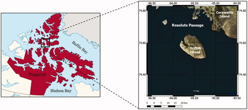
Over the selected study area, 31 RADARSAT-2 Fine Quad Wide (FQW) acquisitions were obtained during September-December 2017 period. A list of the acquisitions sorted by imaging modes is presented in Table 1. Each acquisition encompassed 2 frames, so, a total of 62 frames were used. The acquired SAR images come from different imaging modes ranging from FQ7W to FQ21W, revealing a radar incidence angle difference of about 14.2^°. Using the same dataset, it was demonstrated in Shokr and Dabboor (2020) that the effect of this incidence angle range on the calibrated backscatter is negligible.

Table 1. The 31 RADARSAT-2 acquisitions used in the study, sorted by beam mode.

Beam	Incidence angle		Date (YYYMMDD)
	Near	Far
FQ7W	24.9°	28.3°	20170927
FQ7W			20171021
FQ7W			20171114
FQ8W	26.1°	29.4°	20170920
FQ8W			20171014
FQ8W			20171107
FQ8W			20171201
FQ8W			20171225
FQ10W	28.4°	31.6°	20171007
FQ10W			20171031
FQ10W			20171218
FQ12W	30.6°	33.7°	20170930
FQ12W			20171024
FQ12W			20171117
FQ12W			20171211
FQ13W	31.7°	34.7°	20171110
FQ13W			20171204
FQ13W			20171228
FQ14W	32.7°	35.7°	20170923
FQ14W			20171017
FQ15W	33.7°	36.7°	20171010
FQ15W			20171103
FQ15W			20171127
FQ15W			20171221
FQ16W	34.8°	37.6°	20171003
FQ16W			20171120
FQ16W			20171214
FQ17W	35.7°	38.6°	20171027
FQ18W	36.7°	39.5°	20171123
FQ20W	38.6°	41.3°	20171130
FQ21W	39.5°	42.1°	20171207

Theoretical background

Scattering mechanisms from sea ice types

Radar scattering from natural surfaces is triggered through four known mechanisms; single-bounce (SB) (also known as odd or surface scattering), double-bounce (DB), random multiple-bounce (MB) (also known as volume scattering) and helix scattering. Sea ice may trigger one or more of the first 3 mechanisms (Figure 2), while helix scattering is relevant to complicated man-made structures in urban areas. SB is triggered by smooth or rough surface when the Root Mean Square (RMS) height of the roughness scale is smaller or of same order of magnitude as the incident radar wavelength. The DB mechanism is activated when the signal is bounced twice between two orthogonal surfaces. The MB occurs when the incident wave undergoes many random bounces between numerous scattering elements within the medium. In sea ice, this manifested in ridged/rubble ice surface of bubbly ice volume as found in hummocks of multi-year ice.

Figure 2. Radar backscatter mechanisms from a few sea ice features. (a) single-bounce scattering from leveled ice, (b) double-bounce scattering from ridged ice, (c) multiple-bounce scattering from air bubbles in multi-year ice hummock surface, and (d) another multiple-bounce off the dendritic ice-water interface of very thin snow-free ice layer. h is the thin ice thickness.

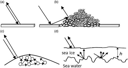
SB and DB mechanisms do not depolarize the incident microwave signal, while the MB does. Therefore, the relative power from the three mechanisms are proxy indicators of the degree of the depolarization of the return signal. This degree, which may be derived from FP or CP observations, can be used to identify certain ice types that contribute heavily to the depolarization of the observed signal such as MYI and very thin ice as demonstrated later.

Polarimetric parameters used in the study

The parameters used in this study are presented in Table 2. Derivation and explanation of the parameters are presented in Appendix A. Throughout the rest of this paper, references to the meanings of those parameters in relation to relevant properties of ice types are made. In this study, we present data from the SPAN because it offers a wider dynamic range than the traditional backscatter coefficients ${\sigma }^o$ (Shokr and Dabboor 2020). The ratio of the MB/SB power ($P_v/P_s$) is presented in the dB scale. Hence, it varies from positive to negative, with positive indication higher MB and vice versa.

Table 2. Polarimetric parameters used in the study.

Parameter	Description	Decomposition method
SPAN	Total backscattering power	–
$H$	entropy	Cloude-Pottier
$A$	anisotropy	Cloude-Pottier
$P_s$	Single-bounce (SB) scattering power	Yamaguchi
$P_d$	Double-bounce (DB) scattering power	Yamaguchi
$P_v$	Multiple-bounce (MB) scattering power	Yamaguchi
$P_v/P_s$	Ratio of MB/SB power in (dB)	–

Physical insight into the scattering mechanisms from sea ice

In this section, we present key aspects of radar scattering mechanisms from different ice type as well as sea water surfaces to demonstrate their use in ice type and OW identification. This physics-based interpretation is augmented with the visual interpretation of SAR images, conducted by ice analysists in the Canadian Ice Service (CIS) to justify and verify the development of the Scat-SeaIce color scheme.

As SB is triggered by smooth or rough surface, it dominates the scattering mechanism of undeformed young and first-year ice. Rafted ice, which usually falls under the category of young ice, does also triggers strong SB for a reason explained in Section 5. The DB scattering is instigated by a dihedral-like surface, which could be manifested in the form of an ice ridge (Figure 2b) or heavy deformed (blocky) surface with appropriate orientation with respect to the incident radar signal. The MB scattering is triggered by one of the following three sea ice features: bubbly sub-surface layer of MYI hummocks, the dendritic interface of thin ice when the radar signal can penetrate the ice cover all the way to the bottom and deformed (blocky) ice surface where the radar signal keeps on bouncing off numerous ice blocks. The first two features are further discussed in the following.

A bubbly layer normally exists within the top 5–20 cm depth of MYI hummocks (Shokr and Sinha 1994) (Figure 2c). The MB scattering power as well as the entropy parameter (see Appendix A) are proportional to the bubble intensity when the bubble size matches the wavelength of the incident signal. As SYI has lower bubble content than MYI (Shokr and Sinha 2015), it can be hypothesized that the MB and the entropy from SYI are less than MYI, provided that the surfaces of both types are equally smooth. However, it is possible that MYI would have a smoother surface as the surface continues to smoothen after each melt season. The above hypothesis has not been tested theoretically or statistically, but first evidences of validity are presented in the case study #2 in Section 4.

The dendritic surface of the sea ice at the ice-water interface is a typical feature of sea ice caused by the non-uniform spatial distribution of the sea water salinity immediately under the ice and the subsequent phenomenon of compositional supercooling (Weeks 2010; Shokr and Sinha 2015). Microwave C-band may penetrate snow-free sea ice to a depth up to 20 cm, depending on the ice bulk salinity (Onstott 1992). This triggers MB scattering at the dendritic interface as shown in Figure 2d. This is demonstrated in a study of thin fast ice (Shokr and Dabboor 2020) and more so in the present data where new ice (NI) was found to be visually identified by its high MB power.

Water surfaces that feature either capillary waves (with wavelength < 17 mm) or no waves are smooth with respect to the much larger wavelength of the incident C-band (5.3 cm). Hence, the scattering mechanism will be strictly SB with mostly specular scattering. When the water surface features gravity waves with a wavelength of a few centimeters under wind speed > 15 km/h, Bragg scattering will be activated and the backscatter increases (LeBlond and Mysak 1981). Nevertheless, the scattering mechanism continues to feature dominant SB. Only large gravity waves or swell that exceeds 1 m may trigger DB mechanisms. Yet, this is not observed in the present dataset.

While some ice types/features demonstrate dominant scattering mechanisms, other types may reveal more than one dominant type such as ice ridges, which could reveal comparable MB and DB mechanisms (Hossain et al. 2014). Moreover, a gradual switch from one dominant scattering mechanism to another mechanism during development of the same ice type may occur. A case to the point is the development of NI from its onset of a few millimeters thick to nilas then gray ice (<15 cm thick). The MB that dominates the scattering during the first few centimeters of growth becomes secondary as the ice thickens because the penetrated C-band signal becomes gradually extinguished within the longer path through the lossy medium of the highly saline NI. This gives rise to more SB scattering.

The above discussions lead to the following summary of contributions of scattering mechanisms from different ice types. They can be used as rules to support the interpretations of the color composite images in the case studies presented in Section 5.

(1) The scattering from the OW surface is strictly SB, whether the surface is smooth or wind-roughened (assuming C-band radar).

1. Thin NI, which is a few centimeters thick, returns dominant MB (volume scattering) triggered by the dendritic ice-water interface. However, this vanishes gradually as ice thickens, allowing for more SB scattering.

2. Level and relatively rough ice surfaces trigger mainly SB scattering with low and high backscatter, respectively.

3. Deformed ice surface triggers high backscatter with SB, MB and perhaps DB in presence of large upturned blocks.

4. The dihedral-shaped ridges may trigger DB scattering.

5. MYI triggers MB scattering power comparable to the SB. However, different scattering mechanisms are revealed upon examining the scattering from hummock and melt pond surfaces as presented in Section 6.

6. The ratio of MB/SB scattering power ($P_v/P_s$) can be used to identify a few ice types, most notably NI and MYI. It can potentially be used to discriminate between MYI and SYI.

7. While the SPAN has nearly equal high value from rough and deformed ice, the $P_v/P_s$ is much higher from deformed ice. This parameter can be used to discriminate between these two types.

Study approach

Operational monitoring of sea ice pursues an age-based ice classification as specified by the World Meteorological Organization (MANICE, 2005). Ice age is then used as a proxy indicator of ice thickness. Linking radar-scattering mechanisms to ice types/features as highlighted in Section 3 has furnished an opportunity to provide scattering-based ice categories. The approach undertaken in this study integrates both concepts. It complements the age-based with scattering-based categorization to resolve issues not identified by the former.

Operational analysis of SAR data adopts visual interpretation of satellite imagery while utilizing auxiliary data including meteorological, climatological, geographic and contextual information. In order to comply with this practice, the approach undertaken in this study focuses on presenting a visual tool to support the operational analysis. The tool integrates polarimetric scattering parameters into a color composite scheme called Scat-SeaIce. The RGB of the color scheme are assigned to the three parameters: SPAN, ($P_v/P_s$) ratio and entropy, respectively. The scenes generated using this color scheme were interpreted against CIS operational regional ice charts or SAR image analysis maps. While colors can be uniquely related to certain ice types and surface features as shown in Section 5, they cannot uniquely identify other age-based ice type. Therefore, dependence on ancillary data should continue within an operational environment.

Operational analysis of SAR images does not take into account the snow effects of snow cover on the observed backscattering. Hence, its effect on the proposed composite color scheme is also neglected. According to a microwave modeling study presented in Nghiem et al. (1995), the MB scattering within dry snow cover, even if metamorphosed into ice grains, is small. Nonetheless, the scattering mechanism from wet, metamorphosed snow or the hoar layer at the base of the snow cover are yet to be determined theoretically or experimentally.

Results

Interpretation of selected polarimetric parameters

Images of the SPAN parameter in addition to six scattering-based polarimetric parameters derived from four RS-2 FP images are presented in Figure 3 along with the associated Scat-SeaIce color composite image. Interpretation of the scenes provide information on how each parameter can be used to support identification of ice types. The SPAN is used in the following discussions as a benchmark to make a first guess of the ice type/feature. The guess is then judged against the power of the observed scattering mechanism.

Figure 3. Images of selected polarimetric parameters (left column) of RS-2 Quad-pol scenes from the days shown at the top row. Marks in the images of 23 November and 11 December are explained in the text.

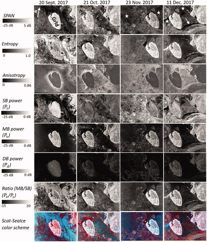
For the scene of 20 September, the records of daily air temperature and wind during the preceding days of 17, 18, 19 and 20 September, showed daily average temperature of −4.2 °C, −8.4 °C, −8.2 °C, and −4.7 °C and daily southeast wind of 22.7 km/h, 34.5 km/h, 12 km/h and 4.2 km/h, respectively. The persistent low temperatures suggest NI rather than OW coverage. Low and high SPAN are observed east and west of Griffith Island (GrId), respectively, and replicated with better contrast in the $P_s$ image. The low SPAN is typical of either calm OW or NI. According to the summary presented in Section 3.3, the high value of the entropy and $P_v$/$P_s$ resolve this situation favoring a decision on NI cover in the eastern area (i.e., in the Resolute Passage). The lower $P_v/P_s$ in the western area indicates the presence of thicker NI or perhaps gray ice (< 15 cm thick). This is the rationale for interpreting the bluish color in the Scat-SeaIce image as being NI. This example highlights the importance of using the $P_v$/$P_s$ as a discriminator between NI and OW. As explained in Appendix A, when the second and third eigenvalues of the coherency matrix, which are used to calculate the anisotropy, are very low, then the anisotropy is considered to be noise. This seems to be the case around the GrId in the scene of 20 September. However, this situation likely arises from grease ice which has only one scattering mechanism (SB) with virtually zero power from the other two mechanisms. Hence, this feature can be used to identify grease ice but more validation of this postulate is needed. If validated, the noisy anisotropic can paradoxically be used to define grease ice.

The scene of 21 October features mainly young seasonal ice types and small areas of open water. Air temperature on that day and the previous 3 days varied between −10 °C and −12 °C and the wind between 6.0 km/h and 29 km/h. The SPAN is lower in the east than the west of GrId. This contrast is confirmed in the SB image, which suggests smoother ice in the east. A few old ice floes can be identified at the bottom of the image based on their high SPAN and elliptical/circular shape within the interstitial of gray and gray-white ice cover. They have low anisotropy, high-volume scattering and high $P_v/P_s.$ The contrast of those floes against the background ice is best visible in the anisotropy image. The red area at the northern tip of GrId appears bright in the SPAN and SB images, which implies that the scattering mechanism is predominantly SB mechanism. This must be rough YI or FYI.

The scene of 23 November features compact ice cover. Strong southwesterly wind prevailed for three days (21–23 November) with daily average between 44.0 km/h and 48.7 km/h. The wind pushed the ice eastward against the fast ice, forming an arch-shaped ridge above Grld, visible in all images except the anisotropy. It also creates deformed ice adjacent to the west coast of GrId crushing the fast ice against the shoreline. High $P_d$ is observed in some parts of the ridge and the deformed ice. A few ice floes are visible in the SPAN, anisotropy, and particularly the $P_s$ images. Those floes appear dark in the anisotropy image with best contrast against the background. The two areas marked by the asterisks in the SPAN image are identified as thin FYI in the CIS interpretation. They both have relatively high entropy and moderately high $P_v/P_s$ ratio and appear with a faint blue shade in the Scat-SeaIce composite image, indicating relatively thick ice.

The scene of 11 December was formed in response to strong wind which blew on 8 and 9 December, with daily average between 45 and 49 km/h. The air temperature remained very cold (<−20 °C) throughout the previous 4 days. The wind broke the ice cover, creating an arch (indicated by the arrow in the SPAN image) with the downstream bands indicating different development stages. They are visible in the SPAN, entropy, $P_s$ and to a lesser extent in the $P_v/P_s$ images. According to the CIS interpretation, the darkest and brightest bands represent OW and gray-white (GW) ice, respectively. The two areas marked by the asterisks in the SPAN image have the same low SPAN but their entropy and $P_v/P_s$ are quite different. The high values of these two parameters designate an area of new (thin) as confirmed in the CIS chart. The low values designate area of undeformed thicker ice, labeled in the CIS chart as thin FYI. Once again, the advantage of using the entropy or the $P_v/P_s$ over the use of the SPAN only to resolve certain ice types is apparent in this case.

Mean values of radar parameters from selected ice/surface types

Mean values of the seven polarimetric parameters shown in Figure 3 were obtained from selected areas of identifiable ice types or surface features and presented in Table 3. It is customary to establish such dataset using homogeneous areas of each type/feature as appear in operational ice charts. While this approach was used, it was complemented with data generated based on interpretation of the scattering mechanisms as outlined in Section 3.3. For example, data about NI type were obtained from areas with $P_v/P_s$ > 0.0 dB rather than ice chart information. This conforms to the methodology of the study (Section 4) to make headway for using the physics of radar/sea-ice interaction within the framework of visual analysis of SAR images. There were no homogeneous areas in the CIS interpretations for either Gray Ice (GI) (10–15 cm thick) or Gray-White Ice (GWI) (15–30 cm thick). Hence, data from both types are combined in the table.

Table 3. Average values of the shown parameters from the given ice types or surface features, calculated from samples provided by CIS interpretation of ice charts or interpretation based on the scattering mechanism.

Parameter/Surface type	SPAN (dB)	Entropy	Aniso-tropy	SB Scat. $P_s$ (dB)	MB. Scat. $P_v$ (dB)	DB scat. $P_d$ (dB)	($P_v/P_s$) (dB)	Source of interpretation
OW – smooth	−12.81	0.30	0.32	−16.47	−23.24	−23.25	−6.77	both
OW – rough	−5.14	0.18	0.45	−8.42	−21.39	−23.79	−12.97	both
NI (<10 cm thick)	−18.83	0.81	0.26	−26.34	−23.80	−29.20	2.54	Scat. Mech.
GI/ GWI	−9.88	0.51	0.39	−14.43	−19.75	−23.97	−5.32	CIS
Rafted ice	−4.54	0.31	0.37	−6.23	−15.17	−22.46	−8.94	both
FYI (smooth)	−9.57	0.25	0.38	−13.67	−21.26	−24.02	−13.26	Scat. mech.
FYI (rough)	−4.32	0.23	0.62	−7.46	−22.45	−22.54	−14.99	both
FYI deformed	−3.89	0.50	0.38	−8.33	−13.78	−19.93	−5.45	both
Ridged ice	−4.44	0.56	0.49	−9.24	−14.64	−18.37	−5.39	Scat. mech
SYI	−5.93	0.51	0.28	−10.61	−14.90	−22.59	−4.29	both
MYI	−5.73	0.56	0.27	−10.82	−13.67	−21.14	−2.88	both

Note. The source of interpretation can be the scattering mechanism, the CIS ice charts or both. The term “both” means that the two sources agree on the ice type/feature within the sampling area.

The number of points from each ice type/feature in the table ranges between 20,000 and 40,000. Anomalies in the data are rejected manually prior to the calculations of the average. A few ice types do not appear in Table 3 such as medium and thick FYI types because they had no homogeneous areas in the ice charts of this dataset and cannot be uniquely identified by their dominant scattering mechanisms. The averages of the backscatter shown in Table 3 for SPAN, SB, DB and MB scattering power were calculated from the values in the linear scale then converted to the dB scale. All values in the table can only be used as a first-order guide to support decisions on ice type/feature because the variability around those values can be high.

A few observations are worth noting from the data in Table 3. While rough OW can have a wide range of SPAN, depending on the wind-roughened surface, the scattering is almost solely triggered by SB mechanism. The $P_v/P_s$ is much negatively lower than that of NI. This feature is used to distinguish OW from NI. The latter has the lowest SPAN (but may not be distinguishable from that of OW) but the highest average $P_v/P_s$ of 2.45 dB. However, the range of this ratio is from −2.0 dB to +4.0 dB. The value decreases progressively as ice thicken. Shokr and Dabboor (2020) used this ratio to estimate thickness of thin ice. GI/GWI have moderate SPAN (−9.88 dB) and entropy (0.51) but can be discriminated from FYI based on $P_v/P_s.$

Although rafted ice has typically smooth surface, with expected low SPAN, Table 3 shows that it has an average SPAN of −4.45 dB with a maximum of −2.45 dB found in this dataset. This anomalous value is explained in Section 6 based on a scenario of scattering that gives rise to both SB and DB mechanisms. Visual analysis of backscatter images is the best approach to identify rafted ice because it incorporates the history of the ice cover and the recent wind data. However, as shown in the case study 5 below, the Scat-SeaIce color scheme depicts this anomalous situation of rafted ice in bright red color.

The rough ice (RI) surface has remarkably high SPAN but this is engendered strictly by surface scattering. Hence, $P_v/P_s$ is negatively high, which makes it easy to discriminate this surface from the MYI with its negatively low values. Deformed ice (DI) constitutes upturned ice blocks that may extend over a relatively large area and represent navigational hazard for marine operations, depending on the ice block size. While the SPAN is equally high from DI and RI surfaces, hence cannot be used to discriminate between them, ${\mathrm{P}}_v,$ entropy, $P_v/P_s$ and to some extent $P_d$ are remarkably higher from DI. Those parameters can be used as discriminators between DI from RI in SAR images.

Ridged ice has SPAN comparable to values from a few other ice types. However, it can be discriminated by its highest DB scattering power (−18.37 dB). More on this point is presented in Section 6. MYI and SYI have nearly the same SPAN but they can be discriminated based on $P_v/P_s$ as rationalized in Section 3.3. The average $P_d$ from MYI is −21.14 dB but it can be higher at locations of hummocks as discussed in Section 6. The Anisotropy from MYI or SYI is the lowest among the examined surfaces (around 0.27 as shown in Table 3). A threshold of this parameter can be used to estimate the spatial distribution and the area of MYI floes within a given scene.

Color composite scheme for visual interpretation

Case study 1: open water and new ice

Two examples of images acquired on 27 September and 30 September 2017 are presented to show the difference between OW and NI in the Scat-SeaIce color scheme. For the first example (Figure 4a), the daily average temperature during the period 23–27 September varied between −3.5 °C and −5.6 °C with strong wind (>35 km/h) prevailed on 26 and 27 September. The wind generated rough water surface, which triggered a relatively high SPAN of −5.12 dB. The scattering is composed primarily of SB mechanism (−8.42 dB) with low entropy (0.18) and low $P_v/P_s$ (−13.0 dB). This renders the surface to appear in red in the Scat-SeaIce image. In general, as water surface triggers only SB mechanism, its reddish shade in this color scheme should be proportional to wind-generated surface roughness; brighter for rough surface and vice versa. Admittedly, same color shades can be associated with smooth and rough FYI surfaces, respectively. Hence, weather data and contextual information become important to discriminate OW from FYI. NI appears bluish or greenish in the Scat-SeaIce because it has high secondary scattering mechanism (MB) as explained in Section 3.1, which triggers high entropy and $P_v/P_s$ (Table 3). The pink strips in the image (a mix of red and blue) indicate high SPAN and high Entropy, which probably represent crushed gray ice as proposed by CIS interpretation.

Figure 4. Scat-SeaIce composite color of a scene acquired by RADARSAT-2 FP mode on (a) 27 September 2017 and (b) 30 September 2017, with surface types labeled according to the CIS interpretation. The inset is the SPAN image. The labels with “?” means the call was made with less certainty by CIS. The yellow asterisks point to gray ice with smooth surface.

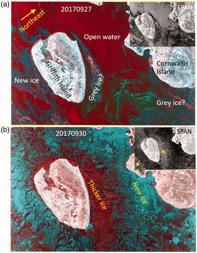
Gradual drop of the daily average air temperature from −4.3 °C on 27 September to −11.7 °C on 30 September suggests formation of thin ice cover in the scene of 30 September (Figure 4b). Daily average wind on 29 and 30 September was 24.5 km/h and 18.5 km/h, respectively, which suggest mechanical ice thickening in some parts. The bluish/greenish tone in Figure 4b represents NI. This cannot be unequivocally confirmed in the low SPAN areas in the figure because it can also be triggered by smooth OW surfaces. The NI is confirmed by its color in the Scat-SeaIce image because its entropy and $P_v/P_s$ are both high (0.71 and 0.70 dB, respectively) while the SPAN is quite low (−15.45 dB). The reddish tone is thicker ice with its higher SPAN as marked by the asterisks in the SPAN image. The SPAN varies around −11.12 dB while the entropy and $P_v/P_s$ are 0.42 and −8.28 dB, respectively. This renders the color to be dark red, confirming the smooth ice surface. Admittedly, this color shade is also shared by smooth FYI. However, the image acquisition time (early October) resolves the ambiguity as it is impossible for the local ice to grow into mature FYI at that time. This, once again, emphasizes the importance of using climatological information to support the interpretation of SAR images, including the Scat-SeaIce color images.

Case study 2: second-year and multi-year ice

For the scene of 14 October (Figure 5a), the daily average air temperature on that day and the previous four days remained constant around −15 °C. According to the CIS interpretation, the scene encompasses 3 sets of floes labeled GWI, MYI, and SYI. While ice floes within those types have similar shapes (nearly rounded), their different colors must be considered as an indicator of difference between their scattering, hence properties. The GWI with its reddish color means high SPAN from a relatively rough surface with small entropy and $P_v/P_s.$ SYI appears with darker reddish tone than MYI, which appears pinkish. Physically speaking, SYI has fewer bubbles in the sub-surface layer than MYI (rationale is presented within an explanation of bubble formation mechanism in Chapter 2 in Shokr and Sinha 2015). Therefore, less volume scattering, entropy and $P_v/P_s$ are expected from SYI. This explains its more reddish (less pinkish color) color shade. In this image the SPAN from the MYI and SYI are −5.19 dB and −6.03 dB, respectively and the ratio $P_v/P_s$ is −2.8 dB and −6.41 dB, respectively. From this image, it appears that the different color shade of MYI and SYI in the Scat-SeaIce scheme can be used as a discriminator criterion. However, this preliminary observation must be confirmed using other datasets. Forward scattering models can also be used to ascertain the less volume scattering from SYI. Since FYI is not possible on the day of acquisition of this image (14 October), it is possible that some of the dark red floes at the left side of the image (especially those with angular boundaries) are locally grown GWI ice with smooth surface.

Figure 5. Scat-SeaIce composite color of a scene acquired by RADARSAT-2 FP mode on (a) 14 October 2017 and (b) 1 December 2017, with surface types labeled according to the CIS interpretation. The inset is the SPAN image.

Case study 3: a scene that combines different ice types

The scene acquired on 1 December 2017 is shown in Figure 5b. The air temperature on that day and the previous 3 days did not exceed −9 °C but the wind on 28–30 November was strong with daily average around 40 km/h. It pushed the ice eastward against the fast ice. The blue band in the image is a fracture with refrozen (new) ice. Red areas around the blue band represent rough ice with dominant BS scattering mechanism. Fast ice appears dark because of its smooth surface, which generates specular SB scattering. GI east of the GrId appears slightly bluish because it is already thicker than 10 cm while the adjacent thicket GWI appears reddish, yet both assume a dark tone because of their smooth surface. MYI floes appear as pinkish as the surrounded deformed ice.

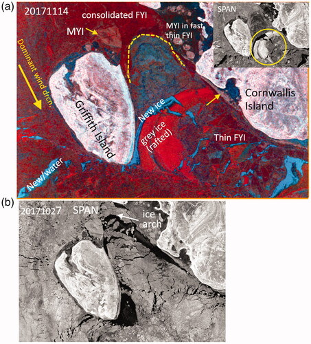
Case 4: thin ice and rafted ice

The image of 14 November (Figure 6a) is a scene following windy days on 11 and 13 November with wind gusted to 45 km/h. It shows an ice arch marked by the dashed yellow line, which appeared for the first time in the image of 27 October (Figure 6b) as a result of strong wind averaging 51 km/h on the previous day. The arch remained at the same location for the rest of the present dataset. It prompted the formation of consolidated ice cover upstream of it, which is labeled in the CIS chart as fast ice. It shows with dark red appearance, implying a smooth surface. The bluish color downstream the arch means thinner ice, which constituted a polynya-like area. At some point in time between 10 and 14 November, which could not be determined because of the gaps between the satellite overpasses, the wind caused extensive ice rafting, depicted as wide red band in Figure 5a. This is identified in CIS chart as gray ice. The SPAN within this band is remarkably high (−1.15 dB) with very low entropy (0.29) and low (negative) $P_v/P_s$ of −9.26 dB. This means dominance of the SB scattering from this rafted ice area. Rationalization is presented in Section 6. The blue areas in Figure 6a are confirmed to be NI in the CIS chart. The pinkish MYI floes at the top of the image featured high SPAN (−4.36 dB), medium entropy (0.54), and low negative $P_v/P_s$ ratio of −2.7 dB. The arrow at the right side of the image points to a shear ridge/deformed ice. It appears in the same color as of the MYI floes.

Figure 6. (a) Scat-SeaIce composite color of a scene acquired by RADARSAT-2 FP mode acquired on 14 November 2017 with surface types labeled according to the CIS interpretation. The inset is the SPAN image. The dashed yellow line marked formation of an ice arch. The dominant wind direction from 9-14 November is indicated by the arrow at the top-left. The arrow at the middle right points to a shear ridge. (b) SPAN image of the 27 October 2017 scene showing arch-like structure with a mix of thin ice and broken pieces of gray ice downstream of it.

Discussions

Previous studies suggested that volume scattering (hence entropy) may be affected by the noise floor of the SAR system (e.g., Espeseth et al. 2020; Wakabayashi et al. 2004; Johansson et al. 2018). Those studies indicate that high entropy measure may result from the random noise rather than the random scattering of the authentic signal within the medium. In Johansson et al. (2018), the authors concluded that incidence angles below 35° are needed to keep the signal-to-noise ratio sufficiently high for the scattering entropy to avoid its sensitivity to the noise. According to Table 1, only 7 out of the 31 orbits used in this study were acquired from beam modes that have incidence angle >35°. These are modes PQ16W to PQ21W. In those beams, the angle can be >35° either partly within the swath or fully across the entire swath. This means that for nearly the entire dataset used in this study the incidence angle fulfills the condition set in Johansson et al. (2018) for the noise-free entropy values.

The noise level of RADASAT-2 is between −31.5 dB and − 33 dB for incidence angle 40.6° and between −33 dB and − 35.75 dB for incidence angle around 26°. In order to further examine the possible effect of the system noise on the entropy measurement in the present dataset, the three orthogonal backscatter coefficients ${\sigma }_{hh}^o,$ ${\sigma }_{vv}^o$ and ${\sigma }_{hv}^o$ along with the SPAN, entropy and $P_v/P_s$ were sampled from 2 areas of thin ice in the scene of 20 September 2017. This is the scene that appears in the first column in Figure 3. Thin ice is associated with the lowest average SPAN in the present data set (average of −18.83 dB according Table 3). Table 4 includes measurements from 2 areas in the scene, area 1 is the bluish area west of the GrId and area 2 includes samples from the greenish areas at the top left and bottom right of the image. Data show that the lowest backscatter coefficient ${\sigma }_{hv}^o$ is still higher than the noise level of RADARSAT-2. The study of Espeseth et al. (2020), which highlights the possible contribution of the system noise to the high entropy measurement, is based on very low backscatter from the smooth surface of oil slick on sea water. The new ice generates remarkably higher values because radar signal penetrates the ice and interacts with the convoluted ice/water interface. Table 4 shows also an opposite order of the entropy and $P_v/P_s$ between area 1 and area 2. This leaves no conclusive evidence on which parameter is better related to growth (thickness) of thin ice. This needs a dedicated study on evolution of polarimetric parameters from thin ice, starting from onset of freezing.

Table 4. Orthogonal backscatter coefficients, SPAN and entropy parameters measured from area 1 and area 2 in the scene of 20 September 2017 (see area definitions in the text above).

	${\sigma }_{hh}^o$	${\sigma }_{vv}^o$	${\sigma }_{hv}^o$	SPAN	entropy	$P_v/P_s$
Area 1	−22.77	−23.22	−28.82	−15.32	0.713	0.393
Area 2	−21.62	−21.90	−27.64	−13.68	0.679	1.018

From the viewpoints of climate science and marine operations, MYI is considered as a single entity. However, from the physical compositional viewpoint it is composed of two sub-entities with different physical and radiative properties; hummocks and depressions (also called melt pond ice). Hummock ice is saline-free ice with a bubbly layer within the subsurface and less snow deposit on the surface. Melt pond ice is a bubble-free medium with marginal subsurface salinity (0–2‰) and thicker snow cover. These factors trigger variable spatial distribution of backscatter. For this reason, texture is commonly used to identify MYI. Figure 7, taken from the image of 21 October, reveals this texture in the SPAN image. The contents of the red box shown in this panel is enlarged in the rest of the panels that reveal the seven polarimetric parameters.

Figure 7. A multi-year ice floe as appears in the SPAN image of 20 November 2017 (top-left panel) showing a melt pond in dark tone surrounded by a hummocky surface in bright tone. Images of different scattering parameters of the area marked by the red box in the SPAN image are also shown. Note the different values of each parameter between melt pond (at the core) and surrounding hummock surfaces.

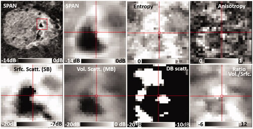
A few observations can be drawn from such a micro-look at this MYI floe. There is a large area of low backscatter in the middle of the segment of the SPAN image, which is interpreted as melt pond ice, surrounded by high backscatter around its boundary, which is interpreted as a hummocky surface. Hummock surface is raised around the melt pond ice surface. As expected, the entropy, SB, MB scattering power as well as the ratio of MB/SB are low from the melt pond compared to the hummocky surface. The striking observations from this figure is the apparent high DB from the hummocky areas around the very low DB from the melt pond ice area. This is conceivable as hummock and melt pond usually coexist next to each other, possibly making dihedral configuration. The contributions of the power from the three scattering mechanisms $P_s,$ $P_v$ and $P_d$ to the total received power from the hummocky perimeter are, −6.0 dB, −8.0 dB and −11.0 dB, respectively. Therefore, the DB scattering power is not negligible from the hummock areas. Therefore, it can be used to map the hummocky surface of MYI. While $P_d$ from MYI averages −21.14 dB (Table 3), the value from the hummock surface is much higher.

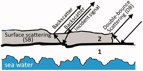
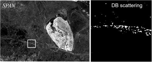
Some rafted ice in the present dataset reveals exceptionally high backscatter as shown in the case study #6 (Figure 6). Figure 8 shows that in addition to the high SPAN from the rafted ice (circled by the ellipse), a relatively high DB scattering power (between −17 dB and −20 dB) also arises. Bailey et al. (2010) presented a one-dimensional thermal consolidation model for rafted ice. They proposed that this ice is composed of two or three layers separated by thin layers of ocean water, which freeze within 15 h. The freezing completes when the thickness of the liquid layer is equal to the surface roughness of the adjacent layer. This configuration is used to explain the coexistence of SB and DB scattering mechanisms from rafted ice as follows.

Figure 8. (a) SPAN image of the 14 November scene showing rafted ice with high SPAN within the ellipse, (b) the DB scattering power ($P_d$), and (c) an enlargement of the area in the white box in (b).

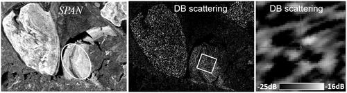
Figure 9 is a graph depicting a rafted ice piece (2) overlying the original ice piece (1). While the original piece has dendrites at the ice-water interface the incident signal may not reach it as the rafted is mechanically thickened. Therefore, no MB scattering is expected at the water interface in this case (note the diminished volume scattering from rafted ice in Table 3). Dendrites at the bottom of piece 2 are removed by friction, so the interface between the two pieces (whether composed of water or ice) becomes smooth, yet with high salinity. It acts as a strong dielectric mismatch, which triggers a strong surface scattering. Based on this configuration, we propose that the radar scattering mechanism from rafted ice is composed of a high SB component and a smaller DB component. The SB component is triggered not only by surface roughness but also by high dielectric medium at the interface between the two ice layers. The DB component is triggered by the raised edge of the rafted piece as shown in Figure 9. The two components contribute to the remarkably high SPAN with its dominant SB scattering. A laboratory experiment is recommended to record the power of the three scattering mechanisms during the first 24 h of the rafting process to confirm the above explanation. In the meantime, the extremely high SPAN can be considered an attribute of rafted ice.

Figure 9. Configuration of the scattering mechanism from rafted ice based on a two-layer model where layer (2) overrides layer (1) with a saline interface (liquid of frozen) between them. Two scattering mechanisms are shown, SB off both top and bottom surfaces of the rafted layer (2), and DB off the dihedral shape of the raised edge of layer (2).

The dihedral-like shape of a ridge is expected to trigger DB scattering mechanism while its blocky ice formation should trigger MB scattering. This is confirmed in the data in Table 3. So far, modeling radar scattering mechanisms from ridged sea ice has not been studied. Nevertheless, Figure 10 shows that, with an appropriate threshold, the DB scattering power can be used to identify ridge pixels easily. The ridge pixels in the enlargement (white pixels) in Figure 10 have the highest DB power (between −14 dB and −18 dB) in this dataset, while the rest of the pixels have nearly constant value around −23 dB. If ridge pixels can be identified based the DB-scattering power, statistics about the number and spatial distribution of ridging in a given area can be obtained. Nevertheless, this requires using a method to connect the ridge pixels and remove possible noise pixels.

Figure 10. SPAN image of 20 November 2017, showing a ridge running across the scene (left). The area within the white box is enlarged in the DP scattering image (right).

While results presented in this paper were obtained from RADARSAT-2 FP SAR mode, this mode is not suitable as a source of SAR data analysis in an operational sea ice monitoring environment. That is because it has a limited swath of a few tens of kilometers with fine spatial resolution better than 10 meters. Operational ice monitoring requires much larger swath with coarser resolution. This is available from the recent SAR configuration of Compact Polarimetry (CP), which offers a near-FP mode capability, yet with wider swath of a few hundreds of kilometers (Raney 2007; Cloude et al. 2012). CP and FP modes are shown to have comparable parameters that express backscatter intensity and scattering mechanisms (Espeseth et al. 2017; Johansson et al. 2018; Dabboor and Geldsetzer 2014; Dabboor and Shokr 2020).

Previous studies have examined the use of CP data, simulated from FP SAR systems, in retrieving sea ice information. A notable study by Geldsetzer et al. (2015) used a dataset of 26 CP parameters simulated from RADARSAT-2 FP system and supported by CIS interpretation to demonstrate their abilities in discriminating several sea ice types and OW in different seasons using an automated classification and a proposed color composite scheme. Other studies that address optimum CP data for computer-assisted methods of ice classification are presented in Dabboor and Geldsetzer (2014) and Dabboor et al. (2018). Zhang et al. (2016) used simulated C-band CP SAR for estimation of the thickness of undeformed sea ice. Dabboor and Shokr (2020) used another set of simulated CP parameters from RADARSAT-2 FP data to model thickness of thin landfast sea ice.

The Canadian Ice Service (CIS) is one of the largest organizational users of SAR data. Currently the visual interpretation of SAR is carried out with dual-pol imagery. As it has been demonstrated that CP imagery has more interpretive potential, it is expected that in the future the operational scheme at CIS will shift from dual-pol to CP. In addition, there are extensive efforts by CIS and other national ice charting organizations into automated classification of sea ice in SAR imagery. The additional information provided by CP promises to aid in the development of these automated classification algorithms. The scattering-based color scheme presented in this study is aimed at utilization in visual analysis of CP data stream.

Conclusions and recommendations

This study uses a set of 62 fully polarimetric (Quad-pol) data from the Wide Fine mode RADARSAT-2 images to explore the potential of using parameters that express the scattering mechanism power in support of operational SAR image analysis. The images were acquired over Resolute Passage area between September and December 2017. The scattering mechanism parameters were calculated from decomposition of the coherency and covariance matrices, both driven from the scattering vectors. The main finding from this study has been the potential use of the power from the radar scattering mechanisms to resolve ice parameters than cannot be resolved using the traditional backscatter information derived from single, dual or fully polarimetric SAR.

As analysis of SAR images in an operational environment is accomplished based on visual interpretation of the images, we developed a color composite scheme to support this process. The scheme, called Scat-SeaIce, combines the total power from the Quad-pol data along with two parameters representing scattering mechanisms, namely the entropy and the ratio between the volume to surface scattering. The three parameters are combined in an RGB color system. Case studies are presented to demonstrate how the color images can be used to infer age-based ice types and surface features. Linking information in the Scat-SeaIce images to ice types and surface features was accomplished using analyst interpretation informed by the regional ice charts produced by the Canadian Ice Service as well as interpretation based on physics of the radar scattering from sea ice. The scattering-based color scheme is introduced as an additional tool to improve results from using the customary age-based visually driven SAR ice information.

Notable benefits from using Scat-SeaIce include unambiguous discrimination between OW and NI, smooth and rough ice surfaces, deformed and ridged ice, and possibility of discrimination between second-year and multi-year ice. The paper introduces quantitative values of power of individual scattering mechanisms from selected ice types. This can be used to develop a quantitative scheme of ice classification but for classes that can be identified by unique scattering mechanisms. Physical insight on scattering mechanisms from selected ice types/features are presented. This includes the difference between scattering parameters from multiyear ice hummocks and depressions, the rafting of young ice, and the ice ridge identification based on the double-bounce scattering power.

It is recommended to continue the process of validating the proposed color scheme using ship observations coincident with polarimetric or compact polarization radar observations. Sea ice data from highly operational areas in southern latitudes such as the Gulf of Saint Lawrence would be particularly interesting because of the potential of the proposed color scheme in resolving thin ice types and open water. Another recommendation is to verify the physical explanation of the high volume-scattering and entropy parameters from newly grown ice using simulated sea ice in a laboratory environment, with measurements from polarimetric scatterometer coincident with ice thickness. This would be the best approach to ascertain the relation between those parameters on one hand and the thin ice thickness on the other hand.

Acknowledgment

The authors would like to thank the anonymous reviewers and the editor for their valuable comments that led to the improvement of the manuscript.

Disclosure statement

No potential conflict of interest was reported by the author(s).

Appendix A: Formulation of the scattering matrices, their decomposition and derived parameters

The scattering matrix $\left[S\right]$ is an array of four complex elements that describe the transformation of the polarization of a wave pulse incident upon a reflective medium $E^i$ to the polarization of the backscattered wave $E^s$ (Lee and Pottier 2009). This is the elementary observation from each pixel in the FP SAR mode. (A-1) $$\left[\begin{array}{c}{E}_h^s\\ E_v^s\end{array}\right]=\mathrm{ }\left[S\right]\left[\begin{array}{c}{E}_h^i\\ E_v^i\end{array}\right]=\left[\begin{array}{cc}{S}_{hh}& S_{hv}\\ S_{vh}& S_{vv}\end{array}\right]\left[\begin{array}{c}{E}_h^i\\ E_v^i\end{array}\right]$$(A-1) Where subscripts $h$ and $v$ refer to horizontal and vertical polarized signals, respectively. It should be noted that the effective backscattering coefficients ${\sigma }_{rt}^o$ in different polarizations are related to the elements of the scattering matrix by the following equations: (A-2) $${\sigma }_{rt}^o=4\pi 〈S_{tr}{S}_{tr}^{\mathrm{*}}〉/A_i$$(A-2) where $A_i$ is the area illuminated by the incident radar pulse, $〈.〉$ denotes the ensemble averages of a number of pixels, subscript $tr$ denote the transmit and receive polarization, and * is the complex conjugate. In the above equation, the scattering element has to be calibrated. Conversion of scattering elements to backscatter coefficient is available in commercial software packages.

Two scattering vectors can be derived from $\left[S\right],$ the lexicological and the Pauli (Lee and Pottier 2009). Assuming the reciprocity condition which implies $S_{hv}=S_{vh},$ the lexicological scattering vector can take the form: (A-3) $${\mathrm{K}}_{\mathrm{L}}={[S_{hh},\mathrm{ }{\mathrm{ }S}_{vv},\mathrm{ }2\mathrm{ }{S}_{hv}]}^T$$(A-3) where the superscript $T$ denotes the vector transpose. An ensemble average of the complex product of the lexicological scattering vector ${\mathrm{K}}_{\mathrm{L}}$ with its complex conjugate transpose ${\mathrm{K}}_{\mathrm{L}}^{\mathrm{*}T}$ leads to what is known as polarimetric covariance matrix [$\mathrm{C}$]. This is a second-order matrix that takes the form (Lee and Pottier, 2019);

(A-4) $$\left[\mathrm{C}\right]=\mathrm{ }〈{\mathrm{K}}_{\mathrm{L}}.{\mathrm{K}}_{\mathrm{L}}^{\mathrm{*}T}〉$$(A-4) On the other hand, the Pauli vector ${\mathrm{K}}_{\mathrm{P}}$ is defined as (A-5) $${\mathrm{K}}_{\mathrm{P}}=\frac{1}{\sqrt{2}}{[{(\mathrm{S}}_{\mathrm{hh}}+{\mathrm{S}}_{\mathrm{vv}},\mathrm{ }{(\mathrm{S}}_{\mathrm{hh}}-{\mathrm{S}}_{\mathrm{vv}}),\mathrm{ }2\mathrm{ }{\mathrm{S}}_{\mathrm{hv}}]}^{\mathrm{T}}$$(A-5)

An ensemble average of the complex product of ${\mathrm{K}}_{\mathrm{p}}$ with its complex conjugate transpose ${\mathrm{K}}_{\mathrm{p}}^{\mathrm{*}T}$ leads to another second-order matrix called polarimetric coherency matrix [$\mathrm{T}$], which takes the form;

(A-6) $$\left[\mathrm{T}\right]=\mathrm{ }〈{\mathrm{K}}_{\mathrm{p}}.{\mathrm{K}}_{\mathrm{p}}^{\mathrm{*}T}〉$$(A-6)

The ensemble averaging in Equations (4) and (6) assumes homogeneity of the scattering medium. The sum of the diagonal elements of $\left[\mathrm{C}\right]$ or [$\mathrm{T}$] corresponds to the SPAN parameter. The eigenvector decomposition of [$\mathrm{T}$] is known as Cloude-Pottier decomposition (Cloude and Pottier 1997). (A-7) $$\left[\mathrm{T}\right]=\left[\mathrm{U}\right]\left[\mathrm{\Lambda }\right]{\left[\mathrm{U}\right]}^{\mathrm{*}T}=\left[\mathrm{U}\right]\left[\begin{array}{ccc}{\mathrm{\lambda }}_1& 0& 0\\ 0& {\mathrm{\lambda }}_2& 0\\ 0& 0& {\mathrm{\lambda }}_3\end{array}\right]{\left[\mathrm{U}\right]}^{\mathrm{*}T}$$(A-7) where [Λ] is the diagonal eigenvalue matrix of $\left[\mathrm{T}\right],$ λ₁ ≥ λ₂ ≥ λ₃ ≥ 0 are the real eigenvalues and $\left[\mathrm{U}\right]$ is a unitary matrix whose columns correspond to the orthogonal eigenvectors of $\left[\mathrm{T}\right].$ Three parameters are derived from the eigenvalues, the entropy $H,$ anisotropy $A,$ and alpha-angle $\alpha ,$ (A-8) $$H=\mathrm{ }-\sum _{\mathrm{i}=1}^3{\mathrm{P}}_{\mathrm{i}}{\log }_3{\mathrm{P}}_{\mathrm{i}}$$(A-8) where ${\mathrm{P}}_{\mathrm{i}}={\mathrm{\lambda }}_{\mathrm{i}}/{\sum }_{\mathrm{i}=1}^3{\mathrm{\lambda }}_{\mathrm{i}}.$ (A-9) $$A=\frac{{\mathrm{\lambda }}_2-{\mathrm{\lambda }}_3}{{\mathrm{\lambda }}_2+{\mathrm{\lambda }}_3}$$(A-9) (A-10) $$\alpha =\mathrm{ }\sum _{\mathrm{i}=1}^3{\mathrm{P}}_{\mathrm{i}}{\mathrm{\alpha }}_{\mathrm{i}}$$(A-10)

The entropy (0 ≤ $H$ ≤ 1) is an indicator of the number of effective scattering mechanisms in the observed backscatter. When $H$ is low, only one deterministic mechanism is expected, either SB or DB. On the other hand, a high entropy indicates strong random scattering (i.e., MB mechanism) with $H$ proportional to the power of MB scattering. For medium values of H, the anisotropy must be examined (0 ≤ A ≤ 1 because ${\mathrm{\lambda }}_2>{\mathrm{\lambda }}_3$). According to Equation (9), the values of $A$ will determine whether there is one or two secondary scattering mechanisms. Low values mean two comparable secondary mechanisms and high values mean one significant secondary mechanism. Note that if both ${\mathrm{\lambda }}_2$ and ${\mathrm{\lambda }}_3$ are very small, the resulting anisotropy can be just noise.

The alpha-angle (0^° ≤ $\alpha$ ≤ 90^°) takes value close to zero when the SB scattering dominates and close to 90° when the DB mechanism dominates, while values between 40° and 50° indicate dipole MB (random) scattering mechanism. For example, if $H$ is very low, $\mathrm{\alpha }$ is needed to determine whether the dominant mechanism is SB or DB. All of the above parameters include proxy information on the type and relative weight of the three scattering mechanisms. The actual power of each mechanism is revealed through the Yamaguchi decomposition parameters.

Yamaguchi decomposition is a four-component model-based polarimetric decomposition (Yamaguchi et al. 2005). This method is based on modeling the covariance matrix $\left[C\right]$ into four scattering matrices corresponding to SB, DB, MB and helix scattering mechanisms. They are denoted by the four subscripts $s,$$\mathrm{ }d,$ $v,$ and $c,$ respectively, in the following equation (Yamaguchi et al. 2005):

(A-11) $$\left[C\right]=\mathrm{ }{f}_s{\left[C\right]}_s+\mathrm{ }{f}_d{\left[C\right]}_d+f_v{\left[C\right]}_v+f_c{\left[C\right]}_c$$(A-11) where $f$ is the weight of the relevant mechanism. In this study, the respective power derived from the coefficient weights of the scattering mechanisms is used. The respective power of SB ($P_s$), DB ($P_d$) and MB ($P_v$) are used.

References

- Bailey, E., Feltham, D.L., and Sammonds, P.R. 2010. “A model for the consolidation of rafted sea ice.” Journal of Geophysical Research, Vol. 115 (No. C4): pp. C004015. doi:https://doi.org/10.1029/2008JC005103.
- Cloude, S.R., Goodenough, D.G., and Chen, H. 2012. “Compact decomposition theory.” IEEE Geoscience and Remote Sensing Letters, Vol. 9 (No. 1): pp. 28–32. doi:https://doi.org/10.1109/LGRS.2011.2158983.
- Cloude, S.R., and Pottier, E. 1997. “An entropy-based classification scheme for land applications of polarimetric SAR.” IEEE Transactions on Geoscience and Remote Sensing, Vol. 35 (No. 1): pp. 68–78. doi:https://doi.org/10.1109/36.551935.
- Dabboor, M., and Shokr, M. 2020. “Compact polarimetry response to modeled fast sea ice thickness.” Remote Sensing, Vol. 12 (No. 19): pp. 3240. doi:https://doi.org/10.3390/rs12193240.
- Dabboor, M., Montpetit, B., and Howell, S. 2018. “Assessment of the high-resolution SAR mode of the RADARSAT constellation mission for first year ice and multiyear ice characterization.” Remote Sensing, Vol. 10 (No. 4): pp. 594. doi:https://doi.org/10.3390/rs10040594.
- Dabboor, M., Montpetit, B., Howell, S., and Haas, C. 2017. “Improving sea ice characterization in dry ice winter conditions using polarimetric parameters from C- and L-band SAR data.” Remote Sensing, Vol. 9 (No. 12): pp. 1270. doi:https://doi.org/10.3390/rs9121270.
- Dabboor, M., and Geldsetzer, T. 2014. “Towards sea ice classification using simulated RADARSAT Constellation Mission compact polarimetric SAR imagery.” Remote Sensing of Environment, Vol. 140: pp. 189–195. doi:https://doi.org/10.1016/j.rse.2013.08.035.
- Dierking, W. 2013. “Sea ice monitoring by synthetic aperture radar.” Oceanography, Vol. 26 (No. 2): pp. 100–111. doi:https://doi.org/10.5670/oceanog.2013.33.
- Ding, F., Shen, H., Perrie, W., and He, Y. 2020. “Is radar phase information useful for sea ice detection in the marginal ice zone?” Remote Sensing, Vol. 12 (No. 11): pp. 1847. doi:https://doi.org/10.3390/rs12111847.
- Espeseth, M.M., Brekke, C., Jones, C.E., Holt, B., and Freeman, A. 2020. “The impact of system noise in polarimetric SAR imagery on oil spill observations.” IEEE Transactions on Geoscience and Remote Sensing, Vol. 58 (No. 6): pp. 4194–4214. doi:https://doi.org/10.1109/TGRS.2019.2961684.
- Espeseth, M.M., Brekke, C., and Johansson, A.M. 2017. “Assessment of RISAT-1 and RADARSAT-2 for sea ice observations from a hybrid-polarity perspective.” Remote Sensing, Vol. 9 (No. 11): pp. 1088. doi:https://doi.org/10.3390/rs9111088.
- Fukuchi, M., Legendre, L., and Hoshiai, T. 1997. “The Canada-Japan SARES project on the first-year ice of Saroma-ko Lagoon (northern Hokkaido, Japan) and Resolute Passage (Canadian High Arctic).” Journal of Marine Systems, Vol. 11 (No. 1–2): pp. 1–8. doi:https://doi.org/10.1016/S0924-7963(96)00022-X.
- Geldsetzer, T., Arkett, M., Zagon, T., Charbonneau, F., Yackel, J.J., and Scharien, R.K. 2015. “All-season compact-polarimetry C-band SAR observations of sea ice.” Canadian Journal of Remote Sensing, Vol. 41 (No. 5): pp. 485–504. doi:https://doi.org/10.1080/07038992.2015.1120661.
- Gill, J.P.S., Yackel, J.J., Geldsetzer, T., and Fuller, M.C. 2015. “Sensitivity of C-band synthetic aperture radar polarimetric parameters to snow thickness over landfast smooth first-year sea ice.” Remote Sensing of Environment, Vol. 166: pp. 34–49. doi:https://doi.org/10.1016/j.rse.2015.06.005.
- Gill, J.P.S., Yackel, J.J., and Geldsetzer, T. 2013. “Analysis of consistency in first-year sea ice classification potential of C-band SAR polarimetric parameters.” Canadian Journal of Remote Sensing, Vol. 39 (No. 2): pp. 101–117. doi:https://doi.org/10.5589/m13-016.
- Gill, J.P.S., and Yackel, J.J. 2012. “Evaluation of C-band SAR polarimetric parameters for discrimination of first-year sea ice types.” Canadian Journal of Remote Sensing, Vol. 38 (No. 3): pp. 306–323. doi:https://doi.org/10.5589/m12-025.
- Hossain, M., Yackel, J.J., Dabboor, M., and Fuller, M.C. 2014. “Application of a three-component scattering model over snow-covered first-year sea ice using polarimetric C-band SAR data.” International Journal of Remote Sensing, Vol. 35 (No. 5): pp. 1786–1803. doi:https://doi.org/10.1080/01431161.2013.879345.
- Isleifson, D., Hwang, B., barber, D., Scharien, R. K., and Shafai, L. 2010. “C-band polarimetric backscattering signatures of newly formed sea ice during fall freeze-up.” IEEE Transactions on Geoscience and Remote Sensing, Vol. 48 (No. 1): pp. 3256–3267.
- Johansson, A.M., Brekke, C., Spreen, G., and King, J. 2018. “X-, C-, and L-band SAR signatures of newly formed sea ice in Arctic leads during winter and spring.” Remote Sensing of Environment, Vol. 204: pp. 162–180. doi:https://doi.org/10.1016/j.rse.2017.10.032.
- Johansson, A.M., King, J.A., Doulgeris, A.P., Gerland, S., Singha, S., Spreen, G., and Busche, T. 2017. “Combined observations of Arctic sea ice with near-coincident colocated X-band, C-band, and L-band SAR satellite remote sensing and helicopter-borne measurements.” Journal of Geophysical Research: Oceans, Vol. 122 (No. 1): pp. 669–691. doi:https://doi.org/10.1002/2016JC012273.
- Kim, J., Kim, D., and Hwang, B. 2012. “Characterization of Arctic Sea Ice thickness using high-resolution spaceborne polarimetric SAR data.” IEEE Transactions on Geoscience and Remote Sensing, Vol. 50 (No. 1): pp. 13–22. doi:https://doi.org/10.1109/TGRS.2011.2160070.
- LeBlond, P. H., and Mysak, L. A. 1981. “Waves in the ocean”, Elsevier Oceanography Series, Elsevier Scientific Publishing Company, Amsterdam, The Netherland, ISBN 0-444-41602-1.
- Lee, J., and Pottier, E. 2009. Polarimetric Radar Images: From Basic to Applications. Boca Raton; London; New York: CRC Press, Taylor and Francis Group. ISBN 978-1-4200-5497-2.
- Moen, M.-A.N., Anfinsen, S.N., Doulgeris, A.P., Renner, A.H.H., and Gerland, S. 2015. “Assessing polarimetric SAR sea-ice classifications using consecutive day images.” Annals of Glaciology, Vol. 56 (No. 69): pp. 285–294.
- Nghiem, S.V., Kwok, R., Yueh, S.H., and Drinkwater, M.R. 1995. “Polarimetric signatures of sea ice 2. Experimental observations.” Journal of Geophysical Research, Vol. 100 (NO. C7): pp. 13681–13698. doi:https://doi.org/10.1029/95JC00938.
- Onstott, R. 1992. “SAR and scatterometer signature of sea ice.” In Microwave Remote Sensing of Sea Ice. Monograph 68, edited by F. Carsey. Washington, DC: American Geophysical Union. ISBN ISBN:97808759003391992).
- Raney, R. K. 2007. “Hybrid-polarity SAR architecture”, IEEE Transactions on Geoscience and Remote Sensing, Vol. 45 (No. 11): pp. 3397–3404.
- Scheuchl, B., Caves, R., Cumming, I., and Staples, G. 2001. “H/A/α-based classification of sea ice using SAR polarimetry.” Proceedings of the 23rd Canadian Symposium on Remote Sensing, 21–24 August 2001, Quebec City, Canada. Canadian Aeronautics and Space Institute, Ottawa, Canada.
- Shokr, M., and Dabboor, M. 2020. “Observations of SAR polarimetric parameters of lake and fast sea ice during the early growth phase.” Remote Sensing of Environment, Vol. 247: pp. 111910. doi:https://doi.org/10.1016/j.rse.2020.111910.
- Shokr, M., and Sinha, N. K. 2015. “Sea ice: physics and remote sensing.” AGU monograph 209, Hoboken, NJ: John Wiley & Sons.
- Shokr, M., and Sinha, N.K. 1994. “Arctic Sea ice microstructure observations relevant to microwave scattering.” ARCTIC, Vol. 47 (No. 3): pp. 265–279. doi:https://doi.org/10.14430/arctic1297.
- Singha, S., Johansson, M., Hughes, N., Hvidegaard, S.M., and Skourup, H. 2018. “Arctic sea ice characterization using spaceborne fully polarimetric L-, C-, and X-band SAR with validation by airborne measurements.” IEEE Transactions on Geoscience and Remote Sensing, Vol. 56 (No. 7): pp. 3715–3734. doi:https://doi.org/10.1109/TGRS.2018.2809504.
- Wakabayashi, H., and Sakai, S. 2010. “Estimation of sea ice concentration in the Sea of Okhotsk using PALSAR polarimetric data.” Proceeding of the International Geoscience and Remote Sensing Symposium (IGARSS’2010), Honolulu, USA, 2398–2401. doi:https://doi.org/10.1109/IGARSS.2010.5652440.
- Wakabayashi, H., Matsuoka, T., Nakamura, K., and Nishio, F. 2004. “Polarimetric characteristics of sea ice in the sea of Okhotsk observed by airborne L-band SAR.” IEEE Transactions on Geoscience and Remote Sensing, Vol. 42 (No. 11): pp. 2412–2425. doi:https://doi.org/10.1109/TGRS.2004.836259.
- Weeks, W.F. 2010. On Sea Ice. Fairbanks, AK: University of Alaska Press.
- Yamaguchi, Y., Moriyama, T., Ishido, M., Yamada, H. 2005. “Four-component scattering model for polarimetric SAR image decomposition.” IEEE Transactions on Geoscience and Remote Sensing. Vol. 45 (No. 8): pp. 1699–1706.
- Zakhvatkina, N., Korosov, A., Muckenhuber, S., Sandven, S., and Babiker, M. 2017. “Operational algorithm for ice–water classification on dual-polarized RADARSAT-2 images.” The Cryosphere, Vol. 11 (No. 1): pp. 33–46. doi:https://doi.org/10.5194/tc-11-33-2017.
- Zhang, X., Dierking, W., Zhang, J., Meng, J., and Lang, H. 2016. “Retrieval of the thickness of undeformed sea ice from simulated C-band compact polarimetric SAR images.” The Cryosphere, Vol. 10 (No. 4): pp. 1529–1545. doi:https://doi.org/10.5194/tc-10-1529.
- Zhang, X., Dierking, W., Zhang, J., and Meng, J. 2015. “A polarimetric decomposition method for ice in the Bohai Sea using C-band PolSAR data.” IEEE Journal of Selected Topics in Applied Earth Observations and Remote Sensing, Vol. 8 (No. 1): pp. 47–66. doi:https://doi.org/10.1109/JSTARS.2014.2356552.