Automated Forest Harvest Detection With a Normalized PlanetScope Imagery Time Series

Abstract

The advent of CubeSat constellations is revolutionizing the ability to observe Earth systems through time. The improved spatial and temporal resolutions from these data could assist in tracking forest harvesting by forest management companies or government organizations interested in monitoring the sustainable management of forest resources. However, differing characteristics of individual satellites in each constellation requires study into geometric and radiometric normalization of the imagery and tuning parameters for change detection algorithms. In this study, a method for the spatial and temporal detection of forest harvest operations using images from the PlanetScope constellation was developed and implemented for a managed forest in Ontario, Canada. Temporal smoothing was applied on Landsat-normalized PlanetScope values of the Normalized Differential Vegetation Index (NDVI), and change points were detected based on the first derivative of the NDVI trend. Detected changes were compared to known locations of harvesting machines. Results indicate that 80–90% of harvested areas were detected, with temporal errors of approximately 9–10 days for two sites. Overall, this study demonstrated that forest harvesting can be detected with relative accuracy, deriving previously unavailable levels of spatial and temporal detail and enhancing the ability of forest stakeholders to monitor the sustainable use of forest resources.

Résumé

L'arrivée des constellations de CubeSat révolutionne la capacité d‘observer les écosystèmes terrestres dans le temps. Les résolutions spatiales et temporelles améliorées de ces données pourraient aider à suivre l‘exploitation des forêts par les entreprises de gestion forestière ou les organisations gouvernementales intéressées par le suivi de la gestion durable des ressources forestières. Cependant, les différentes caractéristiques de chacun des satellites de chaque constellation nécessitent une étude de la normalisation géométrique et radiométrique de l‘imagerie et des paramètres de réglage des algorithmes de détection des changements. Dans cette étude, une méthode de détection spatiale et temporelle des opérations de récolte forestière utilisant des images de la constellation PlanetScope a été développée et mise en oeuvre pour une forêt aménagée en Ontario, Canada. Un lissage temporel a été appliqué aux valeurs PlanetScope normalisées par Landsat de l‘indice différentiel de végétation normalisé (NDVI), et les points de changement ont été détectés sur la base de la dérivée première de la tendance du NDVI. Les changements détectés ont été comparés aux emplacements connus des équipements de récolte. Les résultats indiquent que 80 à 90% des zones exploitées ont été détectées, avec des erreurs temporelles d‘environ 9 à 10 jours pour deux sites. Cette étude a démontré que l‘exploitation forestière peut être détectée avec une précision relative, permettant d‘obtenir des niveaux de détails spatiaux et temporels jusqu’alors inatteignables et d‘améliorer la capacité des parties prenantes à surveiller l‘utilisation durable des ressources forestières.

Introduction

Recent technological advances in spaceborne imaging systems have led to the advent of CubeSats, which are relatively small satellites made up of 10 × 10 × 10 cm units and typically weighing less than 1.5 kg (Heidt et al. 2000). Historically, satellite programs such as the Moderate Resolution Imaging Spectroradiometer (MODIS) onboard the Terra and Aqua platforms have allowed optical daily temporal coverage over the majority of the globe at broad spatial resolutions (ranging from 250 to 1000 m depending on sensor; Justice et al. 2002). Increases in spatial resolution from satellite-based platforms typically require significant tradeoffs with temporal resolution, resulting in fine spatial resolution revisits being at longer temporal scales than their coarser-scale counterparts, typically in the range of weeks to months. The proliferation of CubeSat constellations is revolutionizing the way Earth system processes can be observed through time (Selva and Krejci 2012). In some cases, constellations of hundreds of satellites orbit the Earth in fixed planes, resulting in near-daily coverage at very high spatial resolutions (< 5 m), providing previously unavailable spatial and temporal detail for monitoring ecosystem processes and anthropogenic activities.

Concurrently, the opening of the Landsat archive over a decade ago, has resulted in an expansion of time series analysis approaches, which have exploited the concept of tracking spectral trajectories over time (Wulder et al. 2011, 2012). However, these studies used moderate spatial resolution imagery with temporal resolutions of one to two weeks, meaning that many initial change detection approaches that utilize temporal trajectories have relied on annual best available pixel (BAP) mosaics, such as those used by LandTrendr (Hermosilla et al. 2015; Kennedy et al. 2010) or Composite2Change (C2C; Hermosilla et al. 2015). More recently, with additional moderate spatial resolution platforms such as Sentinel-2, annual time series analysis approaches have moved to sub-annual change detection, using algorithms such as Continuous Monitoring of Land Disturbance (COLD; Zhu et al. 2020). However, these algorithms are limited in how quickly they can detect a change as they require up to six observations (in the case of COLD) before a change event can be automatically detected (Cohen et al. 2020). The advent of CubeSat data offers the potential to allow a near-daily repeat cycle to inform spectral trajectory change analysis and thereby significantly increase the sensitivity of these algorithms to change by tracking finer pixels at finer temporal resolutions over time to inform upon landscape change.

The experience gained by utilizing annual moderate scale resolution mosaics to detect change provides insights into how a spectral trajectory change detection method might be developed for finer spatial and temporal resolution datasets. However, there are a number of differences between the image type and conditions of CubeSat time series data when compared to moderate spatial resolution satellite programs. Notably, in the PlanetScope constellation there are approximately 200 different satellites, resulting in each individual satellite having slightly different spectral calibrations and orbital characteristics (Frazier and Hemingway, 2021). The variable age and characteristics of the sensor network means that these images are not well calibrated to surface reflectance compared to larger satellite programs such as Landsat and Sentinel (Mansaray et al. 2021). Due to variable orbital planes, imagery can be acquired at varying times during the day, under a variety of viewing and sun angle conditions. Due to imagery being gathered by a large number of satellites, geo-rectification of this fine spatial resolution imagery to a consistent map base can be challenging. Additionally, as imagery is acquired by a large number of sensors whose sensitivity characteristics are found to vary, radiometric normalization is needed to provide analysis-ready time series data (Leach et al. 2019). Furthermore, the lack of special spectral sensitivity of many CubeSat cameras (with most being sensitive only to the visible and near-infrared regions of the spectrum) makes preprocessing steps like cloud screening more challenging, resulting in potential noise in the spectral time series (Wang et al. 2021). As a result of these characteristics, the imagery is likely to have more noise and artifacts which are less consistent over space and time, making calibration of imagery a notable challenge before change detection algorithms can be performed.

One environmental application, which would benefit from these increases in spatial and temporal change detection is the field of operational forestry. In many parts of Canada, for example, forest operations continue throughout the year with the requirement of daily tracking of machinery essential to aid in mapping wood extraction, its allocation to the mill, and ultimately how it can be provided to the consumer. The need for chain-of-custody information from the harvesting event through to the consumer requires highly detailed spatial and temporal information to be recorded and, as a result, information on daily timber extraction is critical to ensure sustainable forestry operations. In addition to knowing where individual trees have been harvested, it is also important to understand when this occurred, as this temporal information is key for providing information to mills on the expected timber size and type, as well as to the industry around the weekly supply of timber to the market (Achim et al. 2022).

While forest harvesters enabled with Global Navigation Satellite System (GNSS) receivers can provide much of this information, this is not available on all equipment and is often stored in a variety of formats depending on the manufacturer, making comprehensive databases of forestry equipment movement very challenging to maintain (Söderberg et al. 2021). Additionally, forest operations (particularly in Canada) take place in relatively remote areas with limited or no cellular network connectivity. As a result, there may be delays in relaying harvest machine data to an office or database. If it was possible to observe daily forest operations using a satellite-based change detection approach it would allow larger areas to be monitored independent of the operator, provide valuable information to inform upon sustainable forest management practices, and allow harvest monitoring by government or third-party certification organizations. While PlanetScope imagery has been applied to classify disturbances using imagery before and after the event (e.g., Michael et al. 2018), less is known about how a time series of these images could be used to track the spatial and temporal dynamics of discrete processes such as timber harvesting.

In this paper, we examine the capacity of CubeSat data to track forest operations over a boreal forest environment in central Ontario, Canada throughout a summer harvesting operation. While the high spatial and temporal resolution of PlanetScope images have the ability to derive unprecedented levels of spatial and temporal detail, they require processing to ensure their radiometric consistency through time. This work aims to develop, evaluate, and test a methodology to process these images to enhance their utility in informing sustainable management of forest resources. To do so, we examine the availability of cloud-free CubeSat data over the forest estate, apply preprocessing algorithms to calibrate daily CubeSat data to a consistent spatial and spectral standard, and then modify and apply approaches to detect change across the landscape based on the Normalized Difference Vegetation Index (NDVI; Helman et al. 2015; Hmimina et al. 2013; Lunetta et al. 2006; Tucker 1979), which has been used in previous work monitoring forest change. We assess the performance of the algorithm using a variety of accuracy-based statistics. Once calibrated, we run the algorithm over the forested area and compare it to known harvester locations reported via GNSS. We conclude with a discussion on the reliability of these types of techniques for operational forest management, the challenges associated with processing this data, and recommendations around appropriate time and spatial scales that can realistically be expected from these data sets in an operational framework.

Study area and data

Study area

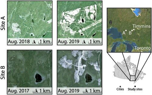
This study was performed on two harvest operations from 2018 and 2019 in the Romeo Malette Forest (RMF) in central Ontario, Canada (Figure 1). The RMF is approximately 630,000 ha, with most of the landbase the focus of forest management operations. Low, poorly drained coniferous stands in the RMF are somewhat common, with elevations ranging from 300 to 320 m above sea level. More common are moderately rolling hills in the southern portion of the RMF with elevations ranging from 305 to 380 m above sea level. Dominant species throughout the forest include balsam fir (Abies balsamea), white birch (Betula papyrifera), eastern larch (Larix laricina), black spruce (Picea mariana), white spruce (Picea glauca), jack pine (Pinus banksiana), trembling aspen (Populous tremuloides), and eastern white cedar (Thuja occidentalis). The climate of the RMF is cool, with a mean January temperature of −17.5 °C and mean July temperature of 17.4 °C. The area has 831 mm annual precipitation, with 313 mm falling as snow (Bazeley et al. 2009; Environment Canada 2022). Within the RMF, two harvest events were chosen so that one could be used to develop models (Site A), while the other (Site B) could be used to demonstrate the application of such models.

Figure 1. Areas of interest within the Romeo Malette Forest in Ontario, Canada. PlanetScope true color imagery shows both areas before and after harvesting.

Optical data

Planetscope

We utilized data acquired from the Dove Classic satellites from the PlanetScope CubeSat constellation, which consists of over 130 CubeSats in sun-synchronous orbit at altitudes of approximately 475 km (Frazier and Hemingway, 2021). The constellation of satellites is such that it provides daily image acquisition globally, at a ground-sample distance of approximately 3 m. Imagery from the constellation archives is available beginning 2016 and is acquired in 4 spectral bands: Blue (455–515 nm), Green (500–590 nm), Red (590–670 nm) and Near-Infrared (780–860 nm). We utilized a total of 295 PlanetScope scenes to observe the two study areas during the summer months (May–September) of their respective years (2018–2019) of harvest activity (Planet Team 2017). Images obtained from the same CubeSat on the same date were mosaiced together to constitute one scene for that day as an initial data preparation step. When multiple images were available from the same day but acquired from different satellites, the images were first independently georectified and radiometrically calibrated to the appropriate Landsat reference scene, and then mosaiced together to constitute the observation for that date, with pixels in overlapping areas taken as that of the higher quality image as reported by the image metadata. For site A, 134 planet images were used which were acquired between April 30 and September 12, 2018. After mosaicking same-date acquisitions, there was complete coverage for 52 days. For Site B, 161 planet images acquired between April 30 and August 25, 2019 were used, which provided coverage on 23 days after mosaicking.

Landsat

In order to radiometrically calibrate the PlanetScope imagery, Landsat Operational Land Imager (OLI) surface reflectance data were downloaded which covered the two areas of interest during their respective observation periods. For calibration of data covering Site A, 9 Landsat scenes were acquired over 5 dates: April 29, May 15, June 16, August 19, and November 14 of 2018. For calibration of Site B data, 3 Landsat scenes were used from May 27, July 14, and September 16 of 2019. In cases where multiple adjacent Landsat scenes from the same date were needed to fully cover the AOI, those scenes were mosaicked together and were considered one scene for the purpose of this study. Landsat bands 2, 3, 4, and 5 corresponding to blue (450–510 nm), green (530–590 nm), red (640–670 nm), and Near-Infrared (850–880 nm), respectively, were used, as these bands best match those acquired by the PlanetScope sensors (Table 1).

Table 1. Characteristics of imagery used from PlanetScope and Landsat Operational Land Imager (OLI) sensors.

Image source	Date range		Wavelengths (nm)
	Site A (2018)	Site B (2019)	Blue	Green	Red	Near Infrared
PlanetScope	April 30–September 12	April 30–August 25	455–515	500–590	590–670	780–860
Landsat OLI	April 29–November 14	May 27–September 16	450–510	530–590	640–670	850–880

PlanetScope images were taken from the “Dove Classic” constellation.

GNSS tracker data

Methods were validated using OpTracker GNSS data obtained from GreenFirst Forest Products. The data was collected using a tablet inside the harvest machinery cabin which runs the OpTracker software (https://www.limgeomatics.com/products/op-tracker). OpTracker takes regular GNSS measurements while the harvest machinery operates, which allows for the area covered by the machinery to be mapped through time. The accuracy of this data is constrained by the GNSS accuracy of the device running the software, which is approximately 3 m for the consumer tablets and phones that were used. The data was stored as a point layer, with each point having attributes including date, time of day, heading, and velocity. A boundary polygon layer was also acquired by digitizing the completed harvest area from aerial photography and was used in the formatting of the validation data.

Methods

In order to develop a calibrated time series of data and extract harvest date predictions four key processing steps were developed, based on Leach et al. (2019), and shown in Figure 2: pre-processing, temporal smoothing and interpolation, breakpoint analysis, and spatial filtering of the resulting change map. Each step is described in detail below.

Figure 2. Workflow for deriving a harvest map from PlanetScope images – pre-processing, temporal smoothing and interpolation, breakpoint analysis, and spatial filtering.

Preprocessing

To detect change using PlanetScope-derived spectral trends, preprocessing is required to reduce noise in the time series signal. There are three primary sources of noise for consideration: (1) cloud, cloud shadow, haze, or smoke present in the imagery, (2) georegistration error, and (3) variation in radiance of the imagery due to the multi-temporal acquisitions occurring with different sensors and under varying lighting conditions.

PlanetScope data includes a useable data mask version 2 (UDM2) as a product after August 2018 (Frazier and Hemingway 2021). The new data mask approach uses machine learning algorithms to classify pixels into one of seven unique categories; clear, cloud, snow, light haze, heavy haze, and anomalous, as well as providing the percent-confidence rating of the classification. While the UDM2 improved on the original classification approach, both masks misclassify cloud, and a visual inspection of the data was used to obtain a reliable time series of imagery.

The PlanetScope imagery available for download has a target geometric accuracy of within 10 m as reported by Planet. This has been confirmed by previous studies, showing the mean error and RMSE to be 2.63 m and 4.80 m, respectively (Dobrinić et al. 2018). Correcting for this error is pertinent to meaningfully tracking the area represented by a single pixel’s change through time. There is a selection of open-source software designed to correct for the registration error in satellite imagery, using either feature-based approaches such Speeded-Up Robust Features (SURF; Bay et al. 2008), or intensity-frequency approaches such as Automated and Robust Open-Source Image Co-Registration Software (AROSICS; Scheffler et al. 2017). Intensity-frequency approaches have the benefit of being able to correct for shifts at the sub-pixel level, and being robust when handling clouds and other significant changes between images.

While the multi-sensor approach of CubeSat Earth imaging allows for new and impressive temporal and spatial resolutions, it calls for a greater need for radiometric normalization (Houborg and McCabe 2018). As the sensors onboard the CubeSats are upgraded with each iteration of launches sustaining the constellation, one area through time will be imaged by a variety of sensors, which can differ in their characteristics and stages of service life. The imaging components of the CubeSats are relatively inexpensive and of lower quality when compared to those of single- or dual-platform satellite missions. Additionally, ground surface lighting and atmospheric conditions vary over the course of an observation period. These challenges have been studied and addressed by previous works such as Leach et al. (2019), who used Landsat data as radiometric reference in order to apply an image-wide linear transformation to PlanetScope imagery observing burned forested areas, and Houborg and McCabe (2018), who used MODIS data to correct for variation in the spectral trends for agricultural monitoring.

In this study, the preprocessing required to prepare the PlanetScope imagery for individual-pixel spectral trend analysis consisted of three steps: initial data cleaning and cloud masking, co-registration of the imagery, and radiometric correction. First, PlanetScope 4-band scenes were downloaded over the area of interest using Planet’s API. All imagery flagged as < 10% cloud was downloaded and Planet’s UDM2 was used to develop a mask, only keeping pixels classified as “clear” and having a confidence of 50% or greater. A visual inspection of the data identified and removed any scenes of low quality in their level of cloud or haze-content that were undetected by Planet’s data mask. Next, to ensure accurate co-registration between imagery, we used AROSICS to co-register all downloaded PlanetScope and Landsat OLI surface reflectance to a common PlanetScope reference scene. The reference scene was selected as one of the existing time series images which was found to be clear and well aligned with its nearest Landsat scene by visual inspection.

Finally, to ensure consistent radiometric normalization of the PlanetScope imagery, the approach of Leach et al. (2019) was applied, which used Landsat-8 scenes overlapping the AOI as spectral reference for calibration of the planet data. Site A used 5 reference Landsat scenes, while site B used 3. The scenes were selected from the PlanetScope archive as those which overlapped the study areas during or near the observation period and which were relatively cloud-free. Each Landsat scene was formatted as a 4-band composite, to match the band combination of the Planet imagery. Then, each of the 52 site A and 23 site B PlanetScope scenes in the time series were paired to its temporally-nearest of the Landsat reference scenes, and the cross-sensor radiometric normalization method outlined in Leach et al. (2019) was applied. The method first uses the Multivariate Alteration Detection (MAD) algorithm (Nielsen, 2002) to detect the most-likely invariant pixels between a given Planet-Landsat scene pairing, temporarily down-sampling the 3 m resolution Planet scene to match the Landsat scene’s 30 m pixel size. Then, pixels passing a no-change probability threshold as defined by MAD are selected, and their spectral values are compared by orthogonal regression to generate a corrective transformation to apply to the full-resolution planet image. We used a threshold of 95% as done by Leach et al. (2019), and in the original application by Canty et al (2004).

Temporal interpolation

Once the Planet data was radiometrically corrected, we derived spectral profiles for each pixel through time. To do so, we calculated the Normalized Difference Vegetation Index (NDVI), a reliable measure of vegetation productivity and health, which has extensively been used to track changes on multitemporal satellite imagery (Helman et al. 2015; Hmimina et al. 2013; Lunetta et al. 2006; Tucker 1979). Despite radiometric normalization, spectral profiles still contain residual noise due to undetected cloud and cloud-shadow, persistent registration error between images, and atmospheric effects, all of which are of common concern in any satellite imagery time series application.

Two temporal filters were used in order to remove noise from the NDVI signal in preparation for changepoint detection. First, we utilized a despiking algorithm modified from Leach et al. (2019) and Kennedy et al. (2010), wherein the observed NDVI value at each timestep is compared to the linearly-interpolated value between its two neighbors. If the central observed value deviates by more than an accepted threshold from the interpolation value, it is replaced by the interpolation value. This despiking filter only corrects large magnitude, ephemeral spikes in the timeseries, arising due to pixels containing cloud or haze which were incorrectly passed through prior masking steps. Given the despiked signal, we then interpolated the data to a daily sampling period, and applied a Savitzky-Golay filter to smooth the data (J. Chen et al. 2004; Savitzky and Golay 1964). The Savitsky-Golay filter implemented with these parameters further smooths the signal, accounting for deviations in radiometry and atmospheric conditions between image acquisitions, without removing important features. A window size of 21 with a polynomial order of 4 provided the level of smoothing required for our purposes without removing important features of the signal.

Breakpoint detection

Breakpoint search methods such as the bottom-up algorithm are used to detect sudden shifts in some time series signal’s value or variability. Modifications to such methods have been shown to be well suited to the application of pixel-wise change detection to moderate-resolution, high signal-to-noise (SNR) satellite imagery time series, such as Landsat BAP composite time series (Hermosilla et al. 2015), which used the bottom-up search method described by Keogh and Smyth (1997) to map landcover change over Canada.

The application of breakpoint analysis for pixel-wise change detection to PlanetScope or other CubeSat imagery is not well studied. Leach et al. (2019) demonstrated the ability of a PlanetScope-derived spectral trend to identify the time of a fire disturbance at a polygon level, but did not use an automated method of breakpoint detection. The application of previously utilized change detection methods to CubeSat time series data at a sub-annual scale is limited by two main factors. The first is the inferiority of the data quality, relative to annual Landsat surface reflectance used in previous studies (e.g., Hermosilla et al. 2015). This difference is characterized by the issues of cloud cover, misregistration, and cross-sensor calibration as described in the preprocessing section above. The second is the influence of phenology on the NDVI time series (Helman et al. 2015) that arises when observing NDVI across seasons. Our approach aims to manage these challenges by utilizing the first derivative (slope) of the spectral trend as a primary metric of change, with properties of the original signal being used for initial classification of pixels and for the selection of the optimal breakpoint from those returned by the search method. To detect change due to harvest in a pixel time series, our approach was as follows:

First, we calculated the slope of the pixel’s spectral trend, to which we applied the Kernelized Change Point Detection (KCPD) implementation of the Pruned Exact Linear Time (PELT) method (Celisse et al. 2018; Figure 2.iii.). The kernelized PELT method returns the optimal breakpoints for a signal given a user defined penalty value. We used a radial basis function kernel, with a penalty value of 4.0. The penalty value was selected by sensitivity analysis covering the range of values (2.5−6.0). The breakpoints in the signal derivative returned by this method correspond to the significant shifts in slope of the spectral trend.

Second, we filtered the breakpoints by attributes of the sub-signals that they separate (Figure 2.iii.). These attributes include: the change in mean slope from one sub-signal to the next, the value of the mean slope of the sub-signal immediately following the breakpoint, the mean of the slope of the entire signal following the breakpoint, and the minimum NDVI value reached in the original signal at any time after the breakpoint. Three minimum NDVI thresholds – values below which a pixel was categorized as “change” – were tested in this analysis (0.25, 0.3, and 0.35). We assumed harvest events to be characterized in a pixel’s spectral trend by a sustained drop in NDVI following the event, with a decline more abrupt than would be observed due to phenological effects. Thus, by an appropriate selection of thresholds applied to the attributes of the signal described above, we can hope to filter out the undesired breakpoints in a pixel’s spectral trend, narrowing the search to those closest to a harvest event. In the case where multiple breakpoints pass the selection criterion, the date that experienced the greatest drop in mean slope (i.e., the most abrupt change in NDVI) was selected and recorded in the raster. To ensure the workflow was applicable across sites, parameterization was performed using only data from Site A, and the selected parameters were applied to Site B.

Spatial filtering

To increase the overall accuracy of the change map, false positives were minimized by applying a sieve filter which removes very small groups of pixels identified as change which consist of fewer pixels than the minimum permissible object size as defined by the user. Groups of pixels smaller than the minimum size are set to the no-data value. After applying a sieve filter of 200 pixels, we then applied a 7 × 7 modal filter to the result, which served to improve the temporal accuracy within identified harvest pixels by homogenizing the date map. The modal filter compares a pixel value (representing a detected breakpoint) with its spatial neighbors and replaces it with the mode, thereby correcting for single pixel anomalies that lie surrounded by presumably more accurate predictions.

Validation

By comparing the prediction layer to the ground truth, we measured the success of the results using the ratios of false positives and false negatives as metrics of spatial accuracy, and the prediction date error, as metric of temporal accuracy. A false positive is defined as a cell for which the prediction layer reports a harvest in conflict with the ground truth, while a false negative is a harvested cell as reported by the ground truth that is missed by the prediction layer. Temporal accuracy was measured as the proximity between the predicted harvest date and the ground truth reported date, and could only be computed for the overlap where both layers report a harvest event at some date. Validation methods were composed of three steps–generating the ground truth layer, counting false positives and negatives, and assessing the temporal accuracy, which are described in detail in the following sections.

Generation of validation dataset

The OpTracker point data was processed to create a ground truth raster for each AOI that could be compared with the harvest date predictions generated by our time series analysis. The OpTracker validation point data was clipped to the study area, and the GNSS points acquired on the same date were converted to lines in the order of their acquisition time. Any clearly erroneous lines, caused by the loss and recovery of the GNSS signal while the harvester moved, were split and deleted manually at this stage. The line data was then buffered by 9 m, and clipped to the boundary polygon layer. A 9 m buffer was selected to account for georegistration error of the GNSS receiver and the distance between the harvester and the cab of the harvester where the GNSS unit was located. The buffered lines were converted to a raster with a 3 m pixel size, to match the spatial resolution of the PlanetScope imagery. Each pixel then contained either the day of year of harvest, or NA if no harvest occurred. Overlapping polygons were handled during rasterization by assigning the conflicted cell the value of the earlier of the overlapping polygon dates.

Accuracy assessment

False positives and negatives were measured as the fraction of a 10,000-pixel sample over the area. The sample was divided to give a proportional selection from harvest and non-harvest regions, based on the ratio of the number of harvested pixels reported by the ground-truth layer to the total number of pixels in the AOI. Then the harvested and non-harvested regions could be randomly sampled with the appropriate sample size. Pixels selected from the harvested region were counted as false negatives if the prediction layer did not contain a date. Likewise, pixels from the non-harvest region were recorded as false positives if the prediction layer reported a harvest. Both counts were divided by the total number of cells sampled from their region to give the ratios of false positivity and negativity within the AOI. The success of the prediction method in identifying harvest is spatially quantified by a low ratio of both false positives and false negatives.

The prediction date error was calculated by subtracting the prediction from the ground truth for each cell where both layers have a date value (i.e., the cells where neither layer is NA). The error was visualized spatially with a raster of prediction date errors and reported as the mean over each study area.

Results

Data availability

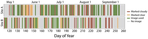
The temporal distribution of PlanetScope images over both sites is shown in Figure 3. Out of the 136 days in the observation period for Site A (April 30–September 12, 2018), 88 days (65%) had images available. 62 days (46%) had images available with <10% cloud. Out of the 117 days in the observation period for Site B (April 30–September 12, 2018), 71 days (61%) had images available, with 39 of those days (33%) having images available with <10% cloud. After visual inspection of this imagery, images with clouds not detected by the PlanetScope algorithm were removed, leaving 52 days with imagery used in Site A (38% of observation period), and 31 days with imagery available in Sie B (26% of observation period). The mean length of time between two clear images in Site A was 2.6 days, with a range from 1 to 12 days. The mean length of time between consecutive clear images in Site B was 3.9 days, with a range from 1 to 15 days.

Figure 3. PlanetScope image availability over the study area for the target year (2018) in Site A. Red bars indicate images with > 10% clouds as determined by the PlanetScope algorithm, while yellow bars indicate images containing < 10% clouds but visually determined to have cloud cover unsuitable for analysis. Green and grey bars indicate days with usable images and no images, respectively.

Parameter selection

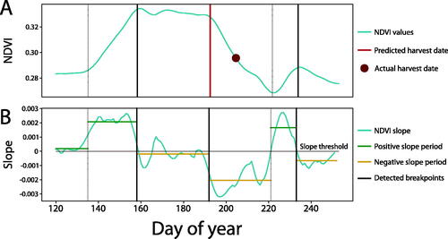
The AROSICS software was run to coregister the available PlanetScope images, achieving registration accuracy of less than a pixel. Once registered, parameterization of minimum NDVI thresholds and breakpoint penalty values were performed on Site A to be applied to Site B. Figure 4 shows the tradeoff between the minimum NDVI threshold value and the breakpoint penalty value for three different simulations under varying parameters in Site A. The importance of a minimum NDVI threshold can be seen in the multiple detected breakpoints in Figure 5, which shows an example of tracking the slope of the temporally smoothed NDVI in a sample pixel. Across minimum NDVI threshold values, there was a tradeoff between temporal and spatial accuracy. The lowest temporal error came with a minimum NDVI threshold of 0.25; however, this threshold also had the highest false positive rates. Conversely, a minimum NDVI threshold of 0.35 had the highest temporal error, but the lowest rate of false negatives. For each minimum NDVI threshold, the false positive and false negative rates were stable across different penalty values. The temporal error exhibited a parabolic trend with the lowest temporal error occurring at penalty values of approximately 4.0. In order to balance the spatial and temporal error, a minimum NDVI value of 0.3 and a penalty value of 4.0 were chosen, giving a temporal error of ∼27 days, false positive rate of ∼30% and false negative rate of ∼33%.

Figure 4. Error analysis for different penalty values and minimum NDVI thresholds in Site A.

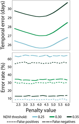
Figure 5. An example of the NDVI values in a single pixel in Site A throughout the growing season. Solid black lines represent significant breakpoints, with the red line as that with the highest probability of being a harvest. Using this method, the predicted harvest date was 8 days earlier than reported by the OpTracker data. The green and yellow lines represent the mean slopes of periods of positive and negative mean slopes, respectively, between breakpoints (vertical lines).

Automated detection

Using the parameters detailed above, pixels were run through an automated detection approach. The OpTracker data showed that 198 ha and 117 ha had been harvested in Sites A and B, respectively, while the detected change from the methods outlined above totaled 181 ha in Site A and 120 ha in Site B. The overall change detection accuracy in Site A was 64.2%, while that of Site B was 79.8% (Table 2).

Table 2. The accuracy of the PlanetScope-based harvest date estimates, reported both temporally and spatially.

		Site A	Site B
Temporal difference (days)	Median	10	9
	Standard deviation	21.1	18.9
	Minimum	0	0
	Maximum	100	90
Spatial difference (% of harvested area)	True positive	77.8%	88.9%

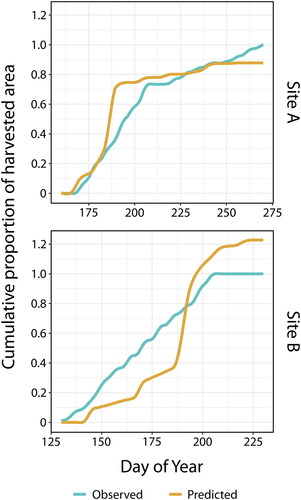
The harvest date as observed by the OpTracker data and predicted by PlanetScope imagery for both sites is shown in Figure 6. The median harvest date in Site A was day 196 (July 15), while in Site B, it was day 170 (June 19). Using PlanetScope imagery, the prediction algorithm detected 77.8% and 88.9% of the total harvested area in Sites A and B, respectively (true positives/total area; Table 2). The predicted harvest date for Site A was generally after the actual harvest (median difference of 5 days after), while that of Site B was generally before the observed harvest date (median difference of 6 days before). Across pixels that were accurately detected as change, the (absolute) median temporal error was 10 days for Site A and 9 days for Site B, with a standard deviation of 21.1 days and 18.9 days for Sites A and B, respectively. The cumulative harvests as observed by the OpTracker data and predicted in this study are shown in Figure 7.

Figure 6. A comparison between the harvest day as observed by the OpTracker data (left) and predicted by PlanetScope (center). The difference (temporal error) is also shown for both sites in the right column.

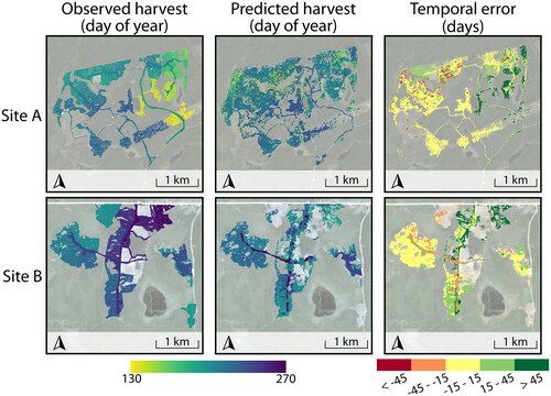
Figure 7. The cumulative proportion of area harvested in both sites, with the blue lines showing the progression of harvest reported by the OpTracker data, and the tan lines showing that of the predictions. The values are a proportion of the total harvested area as reported by the OpTracker data.

Discussion

Data availability and parameterization

While PlanetScope imagery is typically available at daily or near-daily timesteps, clouds and cloud shadows increase the revisit period between subsequent observations of a given area, an example of which is shown in Figure 3. A slower temporal cadence (i.e., > 1 day) could have had an effect on the temporal error in detecting change, as clear observations are required to discern change. The observed temporal resolution of Site A and B was one image every 2.6 and 3.9 days, respectively, with a gap between consecutive images as long as 15 days in Site B. Inconsistent and often long revisit times may have impacted the temporal accuracy of this study, as the breakpoint analysis may have difficulty in determining a change in an irregular time series. If a change occurred over a period of time with no valid observations, a change detection algorithm may have a difficulty in predicting the date of change. Therefore, a denser time series would allow for more certain NDVI trajectories and may reduce the false positive and negative rates. Methods have been proposed to infill data gaps (e.g., Wang et al. 2022) in order to capture long-term trends; however, these can be resource-intensive and may not be able to capture abrupt changes such as those from harvests.

The UDM2 product from PlanetScope uses anomalous brightness values to detect clouds. However, recently harvested pixels with little remaining vegetation will also have anomalous brightness values and may be misclassified as cloud, thereby reducing the number of valid pixels from which to detect a change. With improvements in the UDM2 product and addition of new spectral bands to PlanetScope satellites, this misclassification of clouds may be reduced, and other cloud detection algorithms (e.g., Wang et al. 2021) could be used in order to improve cloud detection.

The minimum NDVI threshold and penalty values selected in this study were found to be optimal based on a perceived balance of their spatial and temporal accuracies. However, the parameters selected may not be optimal for other sites or applications, as the algorithm is influenced heavily by factors such as phenological changes in NDVI, baseline NDVI values, and noise in the time series. Each of these factors will vary notably between sites, thereby altering the algorithm’s parameter-accuracy space. Under the tested range of parameters, the penalty value had little effect on the rate of false positives and negatives, while the minimum NDVI threshold had a stronger effect on error rates. A higher minimum NDVI threshold will admit more breakpoints as potential harvest events, and as such there is a larger likelihood of noise in the signal interfering with the breakpoint selection process leading to a poor breakpoint selection.

Detection accuracy

In general, changes were accurately captured, with 77.8% and 88.9% of harvested areas detected in Site A and Site B, respectively. This is similar to the results of Francini et al. (2020), who used a time series of PlanetScope images to detect harvested areas in Italy and reported detection rates of ∼90%. Although having a different land cover type and input imagery, the accuracy of the current study was similar to that of Han et al. (2020), who reported ∼80–90% overall accuracy of pixel-based change detection algorithms. In this study, changes were generally more accurately detected in the middle of cutblocks, with false positives and negatives occurring toward the edges of a harvest (Figure 6), a pattern that was also noted in Francini et al. (2020). One possibility for the generally lower detection rates on the edges of cutblocks could be edge effects and spectral mixing of border pixels. Object-based change detection has been shown to be effective in high spatial resolution satellite imagery (e.g., Han et al. 2020), and it is possible that region-growing algorithms could be effective in reducing misclassification on edges (Bansal et al. 2022). However, object-based change detection has a number of challenges with continuous values such as NDVI or radiometric inconsistencies such as those seen in PlanetScope imagery (Chen et al. 2012), which were reasons contributing to the choice of a pixel-based change detection approach used in the current study.

The slightly higher detection rates seen in Francini et al. (2020) that of the current study could be attributed to fewer clouds, different harvesting techniques, or an annual time series of images (approximately 4.5 months of imagery in the current study). When an annual time series of imagery is used, a longer trend of a spectral index can be built which may increase certainty around deviations from this trend. While this study monitored forest harvest during the summer months, forest operations in many Canadian jurisdictions take place during the winter. However, a major challenge facing long-term monitoring of the current study are is that of persistent snow cover over winter, which would reflect most incoming solar radiation and therefore obscure the trend of the NDVI slope. In this study, NDVI was selected as the spectral index of interest because of its previous utility in tracking changes in forest condition (Helman et al. 2015; Hmimina et al. 2013; Lunetta et al. 2006). However, there are a variety of other possible spectral indices – such as the Hue Index (Francini et al. 2020) – that could be used, with even more indices possible following the launch of 8-band PlanetScope satellites in 2022.

While this study used PlanetScope scenes with a daily temporal revisit, Planet offers image composites at coarser temporal resolutions (e.g., biweekly or monthly), which typically have lower cloud cover than that of the average scene over a given area. Using a denser time series of images incurs additional computing and storage requirements, but performing such an analysis has the added benefit of increased certainty about the date of change, with the possibility of using these images in a continuous monitoring framework (Coops et al. 2022). For both sites in this study, the average absolute temporal error was approximately 9–10 days, which would likely increase with a decrease in the temporal resolution of the imagery used. Each site had different temporal resolutions of imagery, with Site A having a mean revisit time of 2.6 days, while Site B had a mean revisit time of 3.9 days (Figure 3). The difference in temporal resolution between sites may explain the difference in the differences between observed and predicted harvest dates, as Site A predictions generally preceded harvest dates, while Site B predictions generally followed harvest dates (Figure 7). However, the differences between sites were relatively small (5 days and −6 days for Site A and B, respectively). A temporal resolution such as near-daily PlanetScope imagery can provide valuable information on the temporal dynamics and progression of forest change such as harvesting. Furthermore, knowing change within a 10-day period (as was seen in this study) is a relatively small amount of time, particularly when compared to previous work generating annual maps of forest change from moderate-resolution satellite imagery.

A primary benefit of using data from CubeSats such as PlanetScope is a high spatial and temporal resolution. However, because of spectral inconsistencies and other challenges noted above, it may be beneficial to resample PlanetScope pixels to coarser temporal or spatial resolutions, as long as the coarser spatial resolution was satisfactory for the scale at which the analysis was performed. Performing the analysis at a 9 m spatial resolution, for example, may reduce error in the NDVI values as they are summarized with neighboring cells. While the spatial resolution of such an image would be similar to that of some Sentinel-2 bands (at 10 m), the temporal resolution of PlanetScope images would be much finer, thereby enhancing the ability of these images to discern change with higher temporal precision. When compared to Sentinel-2, the increased temporal resolution from PlanetScope satellites means that there are more chances to get a clear observation of the target surface, thereby suggesting the importance of PlanetScope images in high resolution monitoring of land cover change.

As this work aimed to examine how PlanetScope imagery could be applied to monitor forest harvests, the spatial extent over which the analysis was applied is small relative to the size of forest management units in Canada. If this analysis is applied to broader spatial extents, specifications such as pixel size, parameter selection, data storage, and computer processing power should be considered and adapted in order to balance the accuracy of the results with a reasonable amount of time invested in preparing and processing the data. Furthermore, results of this study indicate that landcover change can be reliably detected using PlanetScope imagery and, as a result, has relevance for disciplines beyond forest management (e.g., mine reclamation; Szostak et al. 2021). Future work in the use of these data for detecting land cover change could use the approach outlined in this study or that of others (e.g., Houborg and McCabe 2018).”

Management implications

A potential use of such a workflow could be in the area of audits or harvest tracking by either forest management companies, government agencies, or third-party certification organizations. Companies interested in tracking machinery and wood allocation at fine temporal resolutions, and government agencies may be able to use PlanetScope time series to understand the spatial and temporal dynamics of harvest activities. GNSS-enabled harvesters have the potential to provide this information, but may not be consistent or robust enough to provide detailed information across harvested areas under different jurisdictions. Furthermore, in jurisdictions (within Canada or internationally) where there is no legal requirement for these devices to be installed, there may not be an incentive to use them. Results from this study show that forest operations can be monitored using an automated change detection approach from high spatial and temporal resolution CubeSat data. Using satellite data to monitor harvests would allow larger areas to be independently monitored, agnostic of the operator, location, or forest type. Such knowledge would provide valuable information to inform upon sustainable forest management practices. The workflow demonstrated above is well-established (e.g., Leach et al. 2019); however, it includes a notable amount of data storage and processing, both of which require knowledge of geospatial analysis tools and pipelines, the expertise of which may not be available at entities interested in harvest tracking.

While this research was performed across two forest stands in the same forest type, the transferability of the spectral normalization and breakpoint detection approach to other forest types (or change in different land cover types) should be feasible as long as consideration is made for input data, smoothing parameters, and change detection algorithms. In order to simplify this processing pipeline for stakeholders, numerous existing algorithms to process the data (e.g., Houborg and McCabe 2018) exist, so attention to the choice of algorithms needs to be made needs to be made. Furthermore, before widespread adoption of these techniques in a forest management context, research and processes need to be standardized in the areas of spectral normalization (Leach et al. 2019), cloud detection (Zhang et al. 2018), and breakpoint detection (e.g., Zhu et al. 2020) of CubeSat data. Analysis-ready and spectrally smoothed PlanetScope data is becoming available using both established and rapidly developing processing algorithms (Houborg and McCabe 2018; Johansen et al. 2022; Wang et al. 2022). While the cost of such analysis-ready products is a consideration to some stakeholders, the availability of temporally dense data at a high spatial resolution is increasing, which is encouraging for future work in using these data for detecting and quantifying land cover change.

Conclusion

Monitoring forest management activities is critical for informing accurate and sustainable use of forest resources. Results from this study demonstrated that relatively accurate change detection can be achieved at high temporal and spatial resolutions through normalization, temporal smoothing, and breakpoint detection of CubeSat images. The high spatial and temporal resolution from CubeSat images such as those available from Planet have the ability to derive previously unavailable levels of detail, thereby enhancing the utility of satellite images in informing sustainable management of forest resources into the future.

Acknowledgements

This analysis was conducted at UBC, which is located on the traditional, ancestral, and unceded land of the xʷməθkʷəy̓əm (Musqueam) people. We thank GreenFirst Forest Products for provision of the forest tractor head GNSS data and enthusiasm for this project, which drove this analysis. Additionally, we thank the anonymous reviewers whose feedback helped to improve and clarify this manuscript.

Disclosure statement

No potential conflict of interest was reported by the author(s).

Additional information

Funding

Components of this research were funded by a NSERC Alliance project Silva21 NSERC ALLRP 556265 − 20, grantee Prof. Alexis Achim and a NSERC Discovery Grant to Coops. This research was partially supported by Natural Resources Canada and the Canadian Wood Fibre Centre through the Forest Innovation Program.

References

- Achim, A., Moreau, G., Coops, N.C., Axelson, J.N., Barrette, J., Bédard, S., Byrne, K.E., et al. 2022. “The changing culture of silviculture.” Forestry: An International Journal of Forest Research, Vol. 95(No. 2): pp. 143–152. doi:10.1093/forestry/cpab047.
- Bansal, P., Vaid, M., and Gupta, S. 2022. “OBCD-HH: an object-based change detection approach using multi-feature non-seed-based region growing segmentation.” Multimedia Tools and Applications, Vol. 81(No. 6): pp. 8059–8091. doi:10.1007/s11042-021-11779-y.
- Bay, H., Ess, A., Tuytelaars, T., and van Gool, L. 2008. “Speeded-Up Robust Features (SURF).” Computer Vision and Image Understanding, Vol. 110(No. 3): pp. 346–359. doi:10.1016/j.cviu.2007.09.014.
- Bazeley, D. G., Morandin, L., and MacIsaac, S. 2009. Contingency Forest Management Plan for the Romeo Malette Forest Timmins District, Northeast Region Tembec Industries Inc. for the 2-year period from April 1, 2007 to March 31, 2009.
- Canty, M.J., Nielsen, A.A., and Schmidt, M. 2004. “Automatic radiometric normalization of multitemporal satellite imagery.” Remote Sensing of Environment, Vol. 91(No. 3–4): pp. 441–451. doi:10.1016/j.rse.2003.10.024.
- Celisse, A., Marot, G., Pierre-Jean, M., and Rigaill, G.J. 2018. “New efficient algorithms for multiple change-point detection with reproducing kernels.” Computational Statistics & Data Analysis, Vol. 128: pp. 200–220. doi:10.1016/j.csda.2018.07.002.
- Chen, G., Hay, G.J., Carvalho, L.M.T., and Wulder, M.A. 2012. “Object-based change detection.” International Journal of Remote Sensing, Vol. 33(No. 14): pp. 4434–4457. doi:10.1080/01431161.2011.648285.
- Chen, J., Jönsson, P., Tamura, M., Gu, Z., Matsushita, B., and Eklundh, L. 2004. “A simple method for reconstructing a high-quality NDVI time-series data set based on the Savitzky–Golay filter.” Remote Sensing of Environment, Vol. 91(No. 3–4): pp. 332–344. doi:10.1016/j.rse.2004.03.014.
- Cohen, W.B., Healey, S.P., Yang, Z., Zhu, Z., and Gorelick, N. 2020. “Diversity of algorithm and spectral band inputs improves Landsat monitoring of forest disturbance.” Remote Sensing, Vol. 12(No. 10): pp. 1673. doi:10.3390/rs12101673.
- Coops, N.C., Tompalski, P., Goodbody, T.R.H., Achim, A., and Mulverhill, C. 2022. “Framework for near real-time forest inventory using multi source remote sensing data.” Forestry: An International Journal of Forest Research. doi:10.1093/forestry/cpac015.
- Dobrinić, D., Gašparović, M., and Župan, R. 2018. “Horizontal accuracy assessment of PlanetScope, RapidEye and Worldview-2 satellite imagery.” International Multidisciplinary Scientific GeoConference: SGEM, Vol. 18(No. 2.3): pp. 129–136.
- Environment Canada 2022. National climate data and information archive. Ottawa, Canada: Environment Canada.
- Francini, S., McRoberts, R.E., Giannetti, F., Mencucci, M., Marchetti, M., Scarascia Mugnozza, G., and Chirici, G. 2020. “Near-real time forest change detection using PlanetScope imagery.” European Journal of Remote Sensing, Vol. 53(No. 1): pp. 233–244. doi:10.1080/22797254.2020.1806734.
- Frazier, A.E., and Hemingway, B.L. 2021. “A technical review of planet smallsat data: Practical considerations for processing and using planetscope imagery.” Remote Sensing, Vol. 13(No. 19): pp. 3930. doi:10.3390/rs13193930.
- Han, Y., Javed, A., Jung, S., and Liu, S. 2020. “Object-based change detection of very high resolution images by fusing pixel-based change detection results using weighted Dempster–Shafer theory.” Remote Sensing, Vol. 12(No. 6): pp. 983. doi:10.3390/rs12060983.
- Heidt, H., Puig-Suari, J., Moore, A., Nakasuka, S., and Twiggs, R. 2000. CubeSat: A new generation of picosatellite for education and industry low-cost space experimentation. In 14th Annual/USU Conference on Small Satellites. UT, USA: Logan.
- Helman, D., Lensky, I.M., Tessler, N., and Osem, Y. 2015. “A phenology-based method for monitoring woody and herbaceous vegetation in Mediterranean forests from NDVI time series.” Remote Sensing, Vol. 7(No. 9): pp. 12314–12335. doi:10.3390/rs70912314.
- Hermosilla, T., Wulder, M.A., White, J.C., Coops, N.C., and Hobart, G.W. 2015. “An integrated Landsat time series protocol for change detection and generation of annual gap-free surface reflectance composites.” Remote Sensing of Environment, Vol. 158 pp. 220–234. doi:10.1016/j.rse.2014.11.005.
- Hmimina, G., Dufrêne, E., Pontailler, J.-Y., Delpierre, N., Aubinet, M., Caquet, B., de Grandcourt, A., et al. 2013. “Evaluation of the potential of MODIS satellite data to predict vegetation phenology in different biomes: An investigation using ground-based NDVI measurements.” Remote Sensing of Environment, Vol. 132: pp. 145–158. doi:10.1016/j.rse.2013.01.010.
- Houborg, R., and McCabe, M.F. 2018. “A Cubesat enabled Spatio-Temporal Enhancement Method (CESTEM) utilizing Planet, Landsat and MODIS data.” Remote Sensing of Environment, Vol. 209: pp. 211–226. doi:10.1016/j.rse.2018.02.067.
- Johansen, K., Ziliani, M.G., Houborg, R., Franz, T.E., and McCabe, M.F. 2022. “CubeSat constellations provide enhanced crop phenology and digital agricultural insights using daily leaf area index retrievals.” Scientific Reports, Vol. 12(No. 1): pp. 5244. doi:10.1038/s41598-022-09376-6.
- Justice, C.O., Townshend, J.R.G., Vermote, E.F., Masuoka, E., Wolfe, R.E., Saleous, N., Roy, D.P., and Morisette, J.T. 2002. “An overview of MODIS Land data processing and product status.” Remote Sensing of Environment, Vol. 83(No. 1–2): pp. 3–15. doi:10.1016/S0034-4257(02)00084-6.
- Kennedy, R.E., Yang, Z., and Cohen, W.B. 2010. “Detecting trends in forest disturbance and recovery using yearly Landsat time series: 1. LandTrendr—temporal segmentation algorithms.” Remote Sensing of Environment, Vol. 114(No. 12): pp. 2897–2910. doi:10.1016/j.rse.2010.07.008.
- Keogh, E.J., and Smyth, P. 1997. “A probabilistic approach to fast pattern matching in time series databases.” Kdd, Vol. 1997: pp. 24–30.
- Leach, N., Coops, N.C., and Obrknezev, N. 2019. “Normalization method for multi-sensor high spatial and temporal resolution satellite imagery with radiometric inconsistencies.” Computers and Electronics in Agriculture, Vol. 164: pp. 104893. doi:10.1016/j.compag.2019.104893.
- Lunetta, R.S., Knight, J.F., Ediriwickrema, J., Lyon, J.G., and Worthy, L.D. 2006. “Land-cover change detection using multi-temporal MODIS NDVI data.” Remote Sensing of Environment, Vol. 105(No. 2): pp. 142–154. doi:10.1016/j.rse.2006.06.018.
- Mansaray, A.S., Dzialowski, A.R., Martin, M.E., Wagner, K.L., Gholizadeh, H., and Stoodley, S.H. 2021. “Comparing PlanetScope to Landsat-8 and Sentinel-2 for sensing water quality in reservoirs in agricultural watersheds.” Remote Sensing, Vol. 13(No. 9): pp. 1847. doi:10.3390/rs13091847.
- Michael, Y., Lensky, I.M., Brenner, S., Tchetchik, A., Tessler, N., and Helman, D. 2018. “Economic assessment of fire damage to urban forest in the wildland–urban interface using planet satellites constellation images.” Remote Sensing, Vol. 10(No. 9): pp. 1479. doi:10.3390/rs10091479.
- Nielsen, A.A. 2002. “Multiset canonical correlations analysis and multispectral, truly multitemporal remote sensing data.” IEEE Transactions on Image Processing : A Publication of the IEEE Signal Processing Society, Vol. 11(No. 3): pp. 293–305. doi:10.1109/83.988962.
- Planet Team 2017. Planet Application Program Interface: In Space for Life on Earth. CA, USA: Planet San Francisco. https://api.planet.com
- Savitzky, A., and Golay, M.J.E. 1964. “Smoothing and differentiation of data by simplified least squares procedures.” Analytical Chemistry, Vol. 36(No. 8): pp. 1627–1639. doi:10.1021/ac60214a047.
- Scheffler, D., Hollstein, A., Diedrich, H., Segl, K., and Hostert, P. 2017. “AROSICS: An automated and robust open-source image co-registration software for multi-sensor satellite data.” Remote Sensing, Vol. 9(No. 7): pp. 676. doi:10.3390/rs9070676.
- Selva, D., and Krejci, D. 2012. “A survey and assessment of the capabilities of Cubesats for Earth observation.” Acta Astronautica, Vol. 74: pp. 50–68. doi:10.1016/j.actaastro.2011.12.014.
- Söderberg, J., Wallerman, J., Almäng, A., Möller, J.J., and Willén, E. 2021. “Operational prediction of forest attributes using standardised harvester data and airborne laser scanning data in Sweden.” Scandinavian Journal of Forest Research, Vol. 36(No. 4): pp. 306–314. doi:10.1080/02827581.2021.1919751.
- Szostak M., Likus-Cieślik J., Pietrzykowski M. 2021. “PlanetScope Imageries and LiDAR Point Clouds Processing for Automation Land Cover Mapping and Vegetation Assessment of a Reclaimed Sulfur Mine.” Remote Sensing, Vol. 13(No. 14): pp. 2717. doi:10.3390/rs13142717.
- Tucker, C.J. 1979. “Red and photographic infrared linear combinations for monitoring vegetation.” Remote Sensing of Environment, Vol. 8(No. 2): pp. 127–150. doi:10.1016/0034-4257(79)90013-0.
- Wang, J., Lee, C.K.F., Zhu, X., Cao, R., Gu, Y., Wu, S., and Wu, J. 2022. “A new object-class based gap-filling method for PlanetScope satellite image time series.” Remote Sensing of Environment, Vol. 280 pp. 113136. doi:10.1016/j.rse.2022.113136.
- Wang, J., Yang, D., Chen, S., Zhu, X., Wu, S., Bogonovich, M., Guo, Z., Zhu, Z., and Wu, J. 2021. “Automatic cloud and cloud shadow detection in tropical areas for PlanetScope satellite images.” Remote Sensing of Environment, Vol. 264: pp. 112604. doi:10.1016/j.rse.2021.112604.
- Wulder, M.A., Masek, J.G., Cohen, W.B., Loveland, T.R., and Woodcock, C.E. 2012. “Opening the archive: How free data has enabled the science and monitoring promise of Landsat.” Remote Sensing of Environment, Vol. 122: pp. 2–10. doi:10.1016/j.rse.2012.01.010.
- Wulder, M.A., White, J.C., Masek, J.G., Dwyer, J., and Roy, D.P. 2011. “Continuity of Landsat observations: Short term considerations.” Remote Sensing of Environment, Vol. 115(No. 2): pp. 747–751. doi:10.1016/j.rse.2010.11.002.
- Zhang, Z., Xu, G., and Song, J. 2018. “CubeSat cloud detection based on JPEG2000 compression and deep learning.” Advances in Mechanical Engineering, Vol. 10(No. 10): pp. 168781401880817. doi:10.1177/1687814018808178.
- Zhu, Z., Zhang, J., Yang, Z., Aljaddani, A.H., Cohen, W.B., Qiu, S., and Zhou, C. 2020. “Continuous monitoring of land disturbance based on Landsat time series.” Remote Sensing of Environment, Vol. 238 pp. 111116. doi:10.1016/j.rse.2019.03.009.