Water Bottom and Surface Classification Algorithm for Bathymetric LiDAR Point Clouds of Very Shallow Waters

Abstract

The absence of accurate point classification limits the effective use of airborne bathymetric LiDAR (ABL) data for coastal zone mapping. In this study, we propose a classification approach using a custom waveform decomposition technique with the pseudo-waveform generated from ABL point cloud data. Initially, the input point clouds were organized into a 2D grid. Next, the points that fall into a grid cell were organized into a histogram using Z-values to generate the pseudo-waveform. Subsequently, the pseudo-waveform was decomposed into water bottom, column, surface, and noise components using a custom multiple Gaussian curve fitting method. The proposed approach was evaluated with datasets acquired in Florida, USA, using a Riegl VQ-880-G ABL system. With an optimized parameter set, the proposed approach achieved F1 score of 98.944% for the classification of water bottom and an overall accuracy of 91.234% for all the classes. Further, the proposed approach was evaluated with datasets acquired in South Korea using a Seahawk system and compared against MBES data, demonstrating that the water bottom was successfully classified with a vertical error of 0.049 ± 0.167 m.

RÉSUMÉ

L'absence de classification précise des nuages de points limite l‘utilisation efficace des données bathymétriques aéroportées LiDAR (ABL) pour la cartographie des zones côtières. Dans cette étude, nous proposons une approche de classification utilisant une technique de décomposition de forme d‘onde personnalisée avec la pseudo-forme d‘onde générée à partir des nuages de points ABL. Initialement, les nuages ​​de points d‘entrée étaient organisés en une grille 2D. Ensuite, les points qui tombent dans une cellule de la grille ont été organisés en un histogramme en utilisant des valeurs Z pour générer la pseudo-forme d‘onde. Par la suite, la pseudo-forme d‘onde a été décomposée en quatre composantes, fond de l‘eau, colonne, surface et bruit, à l‘aide d‘une méthode d‘ajustement de courbe gaussienne multiple personnalisée. L'approche proposée a été évaluée avec des ensembles de données acquis en Floride, aux États-Unis, à l‘aide d‘un système Riegl VQ-880-G ABL Avec un ensemble de paramètres optimisé, l‘approche proposée a obtenu un score F1 de 98,944% pour la classification du fond de l‘eau et une précision globale de 91,234% pour toutes les classes. En outre, l‘approche proposée a été évaluée avec des ensembles de données acquis en Corée du Sud à l‘aide d‘un système Seahawk et comparées aux données MBES, démontrant que le fond de l‘eau a été classé avec succès avec une erreur verticale de 0.049 ± 0.167 m.

Introduction

Over the recent decades, airborne bathymetric LiDAR (ABL) has proven to be an efficient and cost-effective technology for coastal zone mapping. ABL surveying system supports a variety of applications, including sea charting, shoreline mapping, regional sediment management, and benthic habitat mapping (Brock and Purkis 2009; Chust et al. 2010; Kumpumäki et al. 2015; Wedding et al. 2008). ABL differs from airborne topographic LiDAR (ATL) with NIR lasers because it uses a high-power green laser pulse to penetrate water. Also, compared with traditional field wading surveys using GNSS or total station, ABL enables more efficient data acquisition when surveying submerged areas due to its high spatial density and accessibility (Daniele et al. 2019). It is particularly advantageous for measuring shallow water areas inaccessible to a shipborne sonar system owing to navigational safety. Notably, recently developed ABL systems are generally equipped with laser sensors with a high vertical resolution of less than 0.15 m, enabling the measurement of water levels in very shallow areas (Yang et al. 2022). The ability of ABL to penetrate water can be affected by many factors, including energy and length (duration) of laser pulse, flying height, atmospheric conditions, surface turbulence, water clarity and bed reflectivity. In general, the reported penetration depth and vertical accuracy in clear water are 40–60 m and 0.025–0.3 m, respectively (Li et al. 2021). Currently, representative commercial ABL systems include Teledyne Optech CZMIL, Leica Chiroptera, and the Riegl VQ model series. Since 2014, extensive efforts have been devoted by the Ministry of Oceans and Fisheries, South Korea, to the development of a new ABL system, named “Seahawk.” The Seahawk system uses a holographic optical element (HOE) circular scanner that can measure co-registered green and NIR laser beams. The system also uses a real-time computation engine (RTCE) that enables a real-time rendering of the 3D point cloud acquired during the operation to check for missing data (Kim et al. 2019). Since its first successful flight on July 1st, 2018, Seahawk has been widely used to obtain topographic and bathymetric measurements of coastal zones in South Korea. Thus, ABL data is becoming progressively popular among many coastal scientists and engineers for efficient coastal zone mapping and management.

However, the classification of data acquired by ABL systems is challenging because the returned laser beams are a mixture of specular reflections from different water levels, such as the bottom, column, and surface, and backscattering, necessitating a sophisticated data processing method for proper classification (Mandlburger 2020). This is even more difficult in very shallow water, less than 2 m deep, where surface and bottom return pulses are received as merged (Guenther 1985; Pe’eri and Philpot 2007; Schwarz et al. 2019). Several commercial LiDAR processing software tools, such as Terrascan (Terrasolid) and Global Mapper (Blue Marble Geographics 2022), offer point classification functionality. However, these tools were designed for ATL classification and may be unsuitable for water-level classification. Moreover, although they have options that allow the users to manually segment the points, the process is time consuming and laborious. Some manufacturer software tools, such as Leica LiDAR Survey Studio, Riegl RiHYDRO, and Teledyne Optech HydroFusion, offer automatic ABL point classification. However, their algorithms are typically manufacturer-proprietary and, thus, are not open to further scientific studies. Therefore, algorithms and workflows for a straightforward, automated classification of ABL point clouds are needed.

Table 1 summarizes the recent studies on the classification of water bottom and surface using the ABL data. Broadly, the literature can be categorized into waveform-based and point-cloud-based analyses. Often, the full waveform data constitute a mixture of signals reflected from different water levels. Because the recorded signals tend to form Gaussian distribution, many studies attempt to decompose the signals using parametric approaches, such as Gaussian decomposition (Xing et al. 2019; Ma et al. 2019; Yang et al. 2022) or peak detection (Schwarz et al. 2019). Meanwhile, Mader et al. (2019) proposed a full-waveform-stacking method to detect water bottom with weak signal intensity. They organized a grid structure, where all full waveforms of each grid cell were aligned and summed up. In this manner, recurring features with weak signal intensity (i.e., water bottom) were better detectable, and random noise and erratic backscatter effects were reduced within the water column. However, only a few users can access the waveform data. Further, most waveform analyses are focused primarily on detecting peaks, which likely represent the water bottom or surface, from the waveform returns. The point cloud data generated from the waveform analyses, however, often include false positives or negatives in the classification, necessitating a further step to refine the results. Therefore, there have been several attempts to classify water bottom and surface from the point cloud data.

Table 1. Summary of the bathymetric LiDAR classification methods.

Study	Analysis		Classified objects		Methods		Sensor
	Full waveform	Point cloud	Water bottom	Water surface	Parametric approach	Machine learning
Xing et al. 2019	✓	–	✓	✓	✓	–	Mapper5000
Schwarz et al. 2019	✓	–	✓	✓	✓	–	Riegl VQ-880-G
Mader et al. 2019	✓	–	✓	–	✓	–	Riegl VQ-880-G
Ma et al. 2019	✓	–	✓	✓	✓	–	Optech Aquarius
Yang et al. 2022	✓	–	✓	✓	✓	–	Mapper5000
Kogut et al. 2022	–	✓	✓	✓	–	✓	Leica AHAB Chiroptera I
Kogut and Weistock 2019	–	✓	✓	✓	–	✓	Leica AHAB Chiroptera I
Lowell and Calder 2021a	–	✓	✓	–	–	✓	Riegl VQ-880-G
Lowell and Calder 2021b	–	✓	✓	–	✓	✓	Riegl VQ-880-G
Mandlburger et al. 2015	✓	✓	✓	✓	✓	–	Riegl VQ-820-G & VQ-880-G
Yang et al. 2020	–	✓	✓	–	✓	–	Optech Aquarius
Jung et al. 2021	–	✓	✓	–	✓	–	Riegl VQ-880-G

In the literature on the point cloud, supervised machine learning approaches considering a variety of geometric (e.g., depth, x, y, and z) and waveform properties (e.g., intensity, amplitude, and echo width) are often applied. Lowell and Calder (2021a, 2021b) investigated other sources of information to drive non-waveform features, such as scan direction, incident angle, or LiDAR trajectory data, to improve the classification. Once the model is trained, it can be reused to predict the labels for new data. In the literature, commonly adopted machine learning techniques are decision trees (Kogut and Weistock 2019; Lowell and Calder 2021a, 2021b) and neural networks (Kogut et al. 2022).

Although there have been great efforts in facilitating ABL data classification, there are some notable limitations. Machine learning approaches are often data specific and, thus, need to be constantly retrained to make predictions for new data with different characteristics, which requires time-consuming data labeling. To improve data labeling, Lowell and Calder (2021b) produced a preliminary classification using parametric approaches, such as a density-based algorithm and k-means clustering, which are then used as dependent variables for training an extreme gradient boosting machine learning model for a final classification. Approaches to using non-machine-learning methods include that of Mandlburger et al. (2015). They used a ground filtering technique to classify water bottom points, which requires full waveform data for the pre-classification of water levels. Yang et al. (2020) organized point cloud data into grid cells and calculated four sub-regional terrain complexities (slope, standard deviation of depth, Gaussian curvature, and roughness) to determine the adaptive distance threshold for the classification of water bottom. Jung et al. (2021) proposed an inverse histogram approach that solely utilizes the geometric information of point cloud data (i.e., x, y, and z) to classify water bottom. The approach outperformed popular unsupervised learning methods, such as k-means, Otsu, and expectation-maximization algorithms. Unfortunately, these approaches help classify only water bottoms. Further, only a few studies (Schwarz et al. 2019; Yang et al. 2022) attempted to classify very shallow water (<2 m water depth) due to the difficulties of decomposing mixed water levels (i.e., water bottom, column, and surface). In the literature, there is no published work that utilizes point cloud data for the classification of water bottom and surface in very shallow water. Notably, the point cloud data generated from an ABL system tend to include noisy points that are above or below the water levels, leading to over- or under-estimation for the water surface and bottom, respectively. Therefore, although noise filtering is a prerequisite for reliable classification, it has rarely been investigated in the literature. Lastly, as evident from the review (the last column in Table 1), many approaches have been tested and optimized on a single ABL system and not much effort has been exerted to investigate the applicability of the developed approaches with datasets obtained using different ABL systems. To overcome these challenges, we propose an automated and versatile approach that utilizes the pseudo-waveform driven from point cloud data for the classification of water bottom and surface. Specifically, the primary objectives of this paper are to:

• Classify water bottom and surface in very shallow water (<2 m water depth)

• Classify point cloud without waveform and training data

• Investigate the applicability of the developed approach to the datasets acquired by two different systems (Riegl VQ-880-G and Seahawk)

Study area and dataset

In this study, we tested the proposed approach on two independent ABL datasets acquired from Riegl VQ-880-G and Seahawk. The first dataset was used to validate the proposed approach in classifying ABL point cloud data in shallow water, and the second dataset was used to investigate the versatility of the proposed approach on different ABL data and evaluate the classified water bottom points with multibeam echo-sounder (MBES) data. Riegl VQ-880-G (Table A1) data are available from the NOAA National Geodetic Survey (NGS) Remote Sensing Division (NOAA NGS 2016). The test data were acquired from the southern coast of Marco Island, Florida, USA, which is a barrier island in the Gulf of Mexico. Its offshore areas include a sandy substrate and seagrass beds (Weinstein and Heck 1979). Figure 1a and Table 2 show the test site and list details on the VQ-880-G data used in the experiment, respectively. The test data were acquired in very shallow water along the near-shore area. In the table, the Z range of the test data is much larger than the visually measured water depth range due to noise and outliers.

Figure 1. Test site: (a) Marco Island in Florida, USA and VQ-880-G point cloud data and (b) Samcheok in Gangwon-Do, South Korea and Seahawk point cloud data.

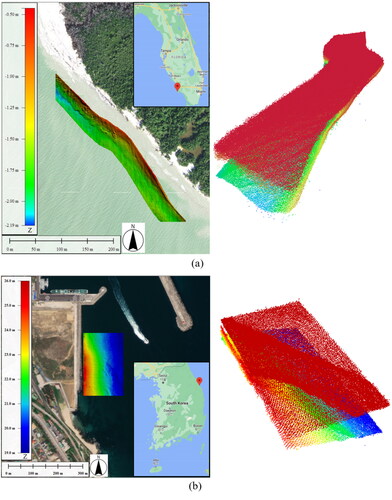
Table 2. Summary of the test datasets.

System	Location	Year	Area (m^2)	Number of points	Point density (pts/m^2)	Z range (m)	Water depth range (m)
Riegl VQ-880-G	Marco Island, Florida, USA	2016	14,192	697,044	49.12	−13.30 ∼ −0.09	0 ∼ 1.81
Seahwak	Donghae, Gangwon-Do, South Korea	2022	40,320	129,125	3.20	18.60 ∼ −26.27	0.30 ∼ 7.28

We performed an additional experiment with data acquired using Seahawk and compared its classified bottom points with MBES data. Detailed specifications and descriptions of the Seahawk system are listed in Table A2. The Seahawk data were obtained from the east coast of Donghae located in Gangwon-Do, South Korea. Because the MBES system cannot be operated in very shallow water, a test region with a wider range of depths (0.30–7.28 m) was selected. Figure 1b and Table 2 show the test site and list the Seahawk data acquisition details, respectively. The eastern coast of the Korean Peninsula, where Donghae is located, is a ridged coast: the bottom of the sea rises and becomes land and has a monotonous coastline and steep incline. The coast has primarily sandy substrate and is undergoing coastal erosion under the influence of waves. Moreover, the tidal difference is small.

Method

A pseudo-waveform can be synthesized by constructing a histogram using the Z values ​​of the point cloud data organized into a regularly spaced 2D grid cells. The elevation and point frequency of the pseudo-waveform are physically similar to the time and amplitude, respectively, of a waveform with a large footprint (Muss et al. 2011). A typical ABL waveform is composed of the multiple signal components returned from the water bottom, column, and surface. When the waveform is decomposed into individual components, the first component is usually classified into the water surface and the last component is the water bottom (Figure 2a). Likewise, when the decomposition is applied to the pseudo-waveform, the components with the highest and lowest Z-values are likely to represent the water surface and water bottom, respectively (Figure 2c). Based on these considerations, we used the ABL pseudo-waveform data for the classification of different water levels, including water bottom, column, and surface. Figure 3 shows the processing steps in the proposed approach. The input point cloud data are organized into a 2D grid to generate a pseudo-waveform for individual cells. Afterward, they are decomposed into Gaussian components through iterative Gaussian curve fitting. Subsequently, the points of each component are classified as water bottom, column, surface, and noise based on the proposed rule-based classification approach.

Figure 2. Examples of (a) waveform decomposition; (b) water levels; and (c) pseudo-waveform decomposition.

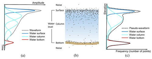
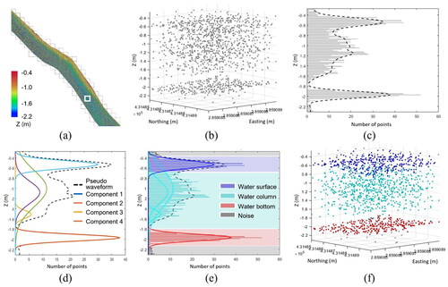
Figure 3. Key steps of the proposed workflow: (a) 2D grid cell structure generation; (b) point cloud that falls onto a single cell; (c) pseudo-waveform generation; (d) pseudo-waveform decomposition; (e) pseudo-waveform classification; and (f) classified point cloud.

Pseudo-waveform generation

Pseudo-waveforms are generated through the following process.

1. The input point cloud data are organized into a 2D grid.

2. The points that fall into a grid cell are organized into a histogram using Z-values.

3. The pseudo-waveform is generated by smoothing the histogram using a Gaussian filter.

4. The process of (2) and (3) is repeated iteratively until all of the cells are visited.

The original point cloud is organized into a regularly spaced 2D grid cell structure using the x and y coordinates. Subsequently, a pseudo-waveform is generated for each cell by organizing the points into a histogram. Note that the cell size (χ) should be large enough to ensure that each cell contains a sufficient number of points to include the water bottom and surface. Smaller cell size allows for greater separation between water bottom and surface but increases the computational cost and leads to an insufficient number of points for each cell. The histogram bin size should be small enough to preserve the details in the vertical variation of the pseudo-waveform. Accordingly, it was empirically set to 0.02 m in this study. Subsequently, Gaussian filtering is performed to smoothen the histogram, enabling a more effective Gaussian curve fitting in the next phase. The effect of smoothing is determined by the standard deviation (σ) of the Gaussian; the larger this is, the histogram generated is smoother, but too large of a value may lead to the loss of details. The optimal value of σ is discussed in Results.

Pseudo-waveform decomposition

A LiDAR waveform is a convolution between a transmitted laser pulse and a surface scattering function, both of which are often considered to follow a Gaussian model (Mallet and Bretar 2009). The received signal through multiple paths generally appears to be a mixture of Gaussian models as defined in Equation (1)(1) $$\mathrm{f}\left(\mathrm{x}\right)=\mathrm{ }\sum _{i=1}^n{A}_i\hspace{0.17em}\exp \hspace{0.17em}\left(-\frac{({x-{\mu }_i)}^2}{2{\sigma }_i^2}\right)$$(1) , where n, A_i, μ_i, and σ_i represent the number of Gaussian models, amplitude, time location, and standard deviation of i-th Gaussian model, respectively. (1) $$\mathrm{f}\left(\mathrm{x}\right)=\mathrm{ }\sum _{i=1}^n{A}_i\hspace{0.17em}\exp \hspace{0.17em}\left(-\frac{({x-{\mu }_i)}^2}{2{\sigma }_i^2}\right)$$(1)

Gaussian modeling is the most widely adopted method for the decomposition of waveform data. In general, prior to fitting multiple Gaussian models, peak detection is performed to determine the number of Gaussian models and their initial locations (Wang et al. 2015; Zhou and Popescu 2017). However, standard multiple Gaussian decomposition may be unsuitable for the ABL waveform due to the attenuation of the echo pulse energy and the overlap of weak echoes (Guo et al. 2017).

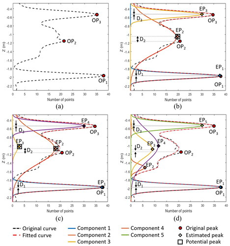
Alternatively, in this study, the generated pseudo-waveforms are decomposed using an iterative Gaussian curve fitting with potential peak (PP) extraction (Kim et al. 2021). This method can improve the decomposition by iteratively estimating PPs through a Gaussian curve fitting in addition to the originally detected peaks. Figure 4 shows the consecutive steps of the proposed approach. The original peaks (OPs) are determined from the local maximum point of the waveform using the peak detection function (findpeaks; MathWorks 2007) in MATLAB (Figure 5a), which returns a set of local maxima (peaks) that is larger than its neighboring samples in the input signal. First, the pseudo-waveform is decomposed into multiple Gaussian components using OPs as initial values. Subsequently, the estimated peaks (EPs) are generated, and the fitness of the Gaussian components is evaluated by the difference (D_i) of Z-values between individual OP_i and their closest EP: if all D_i is less than the Z threshold (τ), the decomposition is considered successful, and the process is terminated. Otherwise, if any D_i is greater than τ, the decomposition is considered inappropriate, and a new decomposition is performed by selecting a PP among the EPs to be added to the new initial values for the Gaussian curve fitting. In Figure 5b, the example shows that D₂ between OP₂ and its nearest EP (EP₂) is greater than τ, such that the algorithm sets EP₂ to PP and performs the second Gaussian curve fitting with OP₁, OP₂, OP₃ and the PP (EP₂). If the third Gaussian curve fitting is required, two PPs are selected in the order of the largest difference in Z-values to the nearest OP among the extracted EPs (Figure 5c), and the next iteration is performed with a total of five initial values (three OPs and two PPs). Note that the PPs are not accumulated according to iteration but are newly determined by increasing the number at each iteration. This process is repeated until all D_i is less than τ (Figure 5d). The smaller the τ value, the more the Gaussian components are generated, resulting in better fitness. However, too small τ can lead to overfitting while increasing the computational complexity. In this study, the τ value was determined through a sensitivity analysis, which will be discussed in the Results section.

Figure 4. Workflow of the pseudo-waveform decomposition.

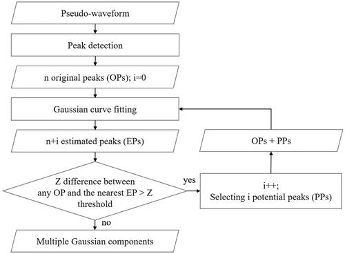
Figure 5. Iterative Gaussian decomposition of pseudo-waveform by estimating the potential peaks: (a) original peak detection; (b,c) estimation of the potential peak through Gaussian curve fitting; (d) pseudo-waveform decomposition result.

Classification

In this phase, the decomposed pseudo-waveform is used to classify the point cloud into four classes, including water bottom, column, surface, and noise. Note that water column and noise are usually not prioritized for classification, but in this study, detection of water column and noise eventually helps separate the water bottom and surface. Assuming that the decomposed pseudo-waveform in a cell includes both water bottom and surface, the points of each cell are classified according to the following rule-based approach.

• The points of the component with the lowest and highest Z-value are classified into water bottom and surface, respectively.

• If more than two components are detected, all the components between the highest and lowest components are classified into the water column.

• Points above the highest component and below the lowest component are left noise.

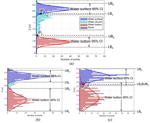
The proposed rule-based classification requires four thresholds: lower bound of the bottom (LB_b), upper bound of the bottom (UB_b), lower bound of the water surface (LB_s), and upper bound of the water surface (UB_s). By default, the bounds of the water bottom and water surface are determined at a 95% confidence interval (CI) (Tan and Tan 2010). If there is an overlap between the two Gaussian curves with the intersection point (IP) closer to the component peak than the 95% CI value, the Z value of the IP is used for the classification bound. For example, in Figure 6a, the IP_s is determined to be LB_s because it is closer to the peak of the water surface component than the 95% CI lower limit, whereas the 95% CI upper limit is determined to be UB_b for the water bottom component because it is closer to the peak of the water bottom than the IP_b. Figure 6b and 6c shows examples of the decomposed, classified pseudo-waveform using the proposed rule-based approach.

Figure 6. Examples of the classification bound determination with (a) four components; (b) two separate components; (c) two intersecting components.

Results

To investigate the feasibility of the proposed approach for classifying pseudo-waveform data, we conducted (1) a sensitivity analysis of the input parameters, a comparative evaluation (2) with existing classification methods, and (3) with the MBES data. For ground-truthing, the acquired ABL data were labeled manually using the classification tool in Terrasolid TerraScan v3.4.

Parameter optimization

The optimal parameters of the proposed approach were determined through a sensitivity analysis of the test variables listed in Table 3. The range of the test variables had been determined from preliminary experimentation. The cell size (χ) should be large enough considering the point density of the ABL data. With a smaller χ, the details of the water bottom topography can be better preserved, but too small a value can lead to not only high computational costs due to the increased number of pseudo-waveforms requiring decomposition but also over-classification for cells with an insufficient number of points. We found that a cell size of smaller than 5 m resulted in very few points in the cells, particularly along the edge of cropped data, and therefore, the test variables were set between 5 and 25 m in 5 m increments. The test variables for the smoothing filter size (σ, standard deviation of the Gaussian filtering) were set between 1 and 4. This value should be large enough to ensure smooth pseudo waveforms, but too large of a value could lead to the loss of important details of the pseudo waveform. Lastly, the test variables for the Z threshold (τ) were set between 0.1 m and 0.5 m in 0.1 m increments. The smaller the value of τ, the more the Gaussian curves are decomposed from the pseudo waveforms, but too small of this value may lead to over-decomposition. A total of 5 × 4× 5 = 100 combinations were investigated for the three parameters (χ, σ, and τ). For evaluation, a pointwise comparison was conducted using the manually labeled point cloud, thereby facilitating several accuracy measurements: the precision, recall, and F1 score for the classification of water bottom and surface, and the overall accuracy for that of all four classes. The following Equations (2 ∼ 5) are utilized for quantitative evaluations, where a true positive (TP) is a classified point that is in the ground truth, a true negative (TN) is a point that is neither in the ground truth nor classified data, a false positive (FP) is a classified point that is not in the ground truth, and a false negative (FN) is a point in the ground truth that is not classified. (2) $$\mathrm{pecision}=\mathrm{ }\frac{\mathrm{TP}}{\mathrm{TP}\mathrm{ }+\mathrm{ }\mathrm{FP}}$$(2) (3) $$\mathrm{recall}=\mathrm{ }\frac{\mathrm{TP}}{\mathrm{TP}\mathrm{ }+\mathrm{ }\mathrm{FN}}$$(3) (4) $$\mathrm{F}1=\mathrm{ }\frac{2\times \text{precision}\times \mathrm{recall}}{\mathrm{Precision}+\mathrm{recall}}$$(4) (5) $$\text{overall accuracy}=\mathrm{ }\frac{\mathrm{TP}\mathrm{ }+\mathrm{ }\mathrm{TN}}{\mathrm{TP}\mathrm{ }+\text{ FN }+\mathrm{ }\mathrm{TN}+\mathrm{ }\mathrm{FP}}$$(5)

Table 3. Test variables for sensitivity analysis.

Parameter	Unit	Test variables
Cell size (χ)	Meters	5, 10, 15, 20, 25
Smoothing filter size (σ)	Unitless	1, 2, 3, 4
Z threshold (τ)	Meters	0.1, 0.2, 0.3, 0.4, 0.5

Efficiency (number of processing points per second) was also calculated to evaluate the computational load with respect to different parameter sets. Note that the time required for loading the point cloud data is not included in the efficiency. The proposed approach was implemented in MATLAB and the experiments were conducted on a computer with an Intel^® Core™ i5-7500 CPU (3.4 GHz, 16 GB RAM). Tables 4 and 5 list the top and bottom 10 combinations of the classification parameters in the descending and ascending order of overall accuracy for the four classes, respectively. The proposed approach achieved the best overall accuracy of 91.234% with the optimized parameter set (χ: 5 m, σ: 2, and τ: 0.3 m). Overall, with a smaller cell size, higher accuracy was achieved because more details of the water bottom topography were preserved. The top 10 combinations in Table 4 tend to have small values of less than 2 for the smoothing filter size as the small size helps preserve the high variability of the pseudo waveform. However, Table 5 shows that the combination of a small filter size (1) and a large cell (20 or 25 m) size can lead to low recall rates due to over-decomposition of the water bottom. Lastly, Tables 4 and 5 show that the proposed approach is less sensitive to the Z threshold in terms of accuracy.

Table 4. Top 10 combinations of parameters in descending order of overall accuracy for VQ-880G data.

Rank	Parameters						Accuracy				Efficiency (1000 points/s)
	Cell size (m)	Filter size	Z threshold (m)	Water bottom			Water surface			Overall accuracy (%)
				Precision (%)	Recall (%)	F1 score (%)	Precision (%)	Recall (%)	F1 score (%)
1	5	2	0.3	99.240	98.649	98.944	81.738	98.715	89.428	91.234	39.815
2	5	2	0.5	99.241	98.649	98.944	81.720	98.716	89.417	91.225	41.963
3	5	2	0.4	99.241	98.649	98.944	81.719	98.716	89.416	91.224	43.707
4	5	2	0.2	99.225	98.345	98.783	81.680	98.603	89.348	91.052	26.877
5	5	2	0.1	99.227	98.214	98.718	81.587	98.506	89.252	90.928	20.215
6	5	1	0.5	99.520	87.899	93.349	85.087	95.908	90.174	88.014	4.450
7	5	1	0.3	99.520	87.907	93.354	85.189	95.727	90.151	88.012	3.837
8	5	1	0.4	99.520	87.899	93.349	85.069	95.899	90.160	88.004	4.459
9	10	2	0.5	98.211	89.259	93.521	82.929	98.381	89.997	87.839	34.762
10	10	2	0.4	98.211	89.259	93.521	82.913	98.381	89.987	87.831	23.614

Table 5. Bottom 10 combinations of parameters in ascending order of overall accuracy for VQ-880G data.

Rank	Parameters						Accuracy				Efficiency (1000 points/s)
	Cell size (m)	Filter size	Z threshold (m)	Water bottom			Water surface			Overall accuracy (%)
				Precision (%)	Recall (%)	F1 score (%)	Precision (%)	Recall (%)	F1 score (%)
1	20	1	0.1	99.070	21.005	34.661	85.744	95.518	90.367	62.747	2.590
2	20	1	0.2	99.057	22.227	36.307	85.395	97.473	91.035	63.641	4.213
3	20	1	0.3	99.254	23.869	38.484	85.202	97.480	90.929	64.211	11.540
4	20	1	0.4	99.182	23.894	38.511	85.296	97.464	90.975	64.260	17.591
5	20	1	0.5	99.183	23.925	38.550	85.310	97.457	90.980	64.279	19.814
6	25	1	0.5	97.324	25.964	40.992	84.903	97.925	90.950	64.799	16.711
7	25	1	0.4	97.324	25.964	40.992	84.942	97.925	90.972	64.818	16.081
8	25	1	0.1	99.179	25.327	40.349	85.624	97.696	91.263	64.938	3.917
9	25	1	0.2	98.837	26.419	41.693	85.305	97.754	91.106	65.190	6.243
10	25	1	0.3	97.678	29.613	45.448	85.180	97.849	91.076	66.299	12.567

Overall, the experimental results demonstrated that the water bottom is more sensitive to the choice of the parameters than the water surface, probably because the water surface has lower variability of Z values compared with the water bottom. Note that, compared with the water bottom, an accurate ground truthing of the water surface is more challenging with ABL data because it is difficult to distinguish the water surface from the water column. Therefore, the accuracy in the water surface classification can be subject to classification bias depending on experts’ knowledge. In this study, the ground truthing of the water surface points was performed conservatively; only the points around the sea level are considered reliable for extraction, ultimately resulting in low precision rates.

Figure 7 depicts the trend of the efficiency and the accuracies with respect to the three parameters. In general, the overall accuracy is more sensitive to the cell size and smoothing filter size compared with the Z threshold. The graph in Figure 7a shows that as the cell size increases, the F1 score of the water surface classification tends to slightly increase while the F1 score of the water bottom classification drastically decreases, ultimately resulting in the lowest overall accuracy at the cell size of 25 m. In Figure 7b, with increasing the smoothing filter, the F1 score of the water surface classification tends to gradually decrease, while the F1 score of the water bottom classification reaches the highest value at the smoothing filter size of 2, and then slightly decreases. Lastly, Figure 7c shows that both the overall accuracy and the F1 scores for the classification of water bottom and surface are less sensitive to the Z threshold.

Figure 7. Sensitivity analysis that accounts for both water bottom and surface with respect to three parameters: (a) cell size; (b) smoothing filter size; (c) Z threshold.

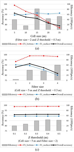
Figures 7b and 7c show that calculation efficiency highly correlates with the smoothing filter size and Z threshold. In Figure 7b, although the best efficiency was achieved with the smoothing filter size of 4, it is desirable to use the filter size of 2 because it shows a good balance between overall accuracy and efficiency. Figure 7c shows that the Z threshold is less sensitive to the overall accuracy, therefore it is recommended to use large Z thresholds. On the other hand, Figure 7a shows that there is no clear trend between efficiency and cell size. This is due to the fact that the computation of the proposed approach is primarily affected by the iterative Gaussian curve fitting in the decomposition process, where the number of original peaks and the number of iterations depends on the smoothing filter size and the Z threshold parameters, respectively. In Figure 7a, although the best efficiency was achieved with the cell size of 15 m, it is recommended to use the cell size of 5 m as it archived the best overall accuracy while maintaining a reasonable efficiency.

Comparative evaluation

The performance of the proposed approach was compared with the classification data provided by NOAA NGS and the existing water bottom classification techniques, which are k-means (Lloyd 1982) and inverse histogram methods (Jung et al. 2021). The ABL data provided by NOAA NGS have the three classification codes of water, water bottom, and noise. The inverse histogram is one of the state-of-the-art approaches, which is specifically designed for the extraction of bathymetric bottom points. The k-means is a simple but effective clustering algorithm that has been used extensively in many applications with multi-dimensional (i.e., 2D or 3D) spatial data. They were chosen for the comparative evaluation because (1) they use point cloud input; (2) they can be readily adapted to our grid cell data structure; and (3) they are parametric approaches that do not require training data. Note that both the inverse histogram and k-means use the presence of a gap between the lowest water column points and the bathymetric bottom for binary classification. Therefore, the comparative evaluation was performed only considering the classification accuracy of the water bottom. Table 6 describes the performance of the four different methods: provided, k-means, inverse histogram, and the proposed approach. The optimized parameter set (χ: 5 m, σ: 2, and τ: 0.3 m) was used for the proposed approach. The k-means method requires user input for the number of clusters, which was set to 2 for binary classification in this study. The inverse histogram approach requires three parameters, which were determined according to Jung et al. (2021). Notably, the water bottom classifications were performed for individual cells created using the same cell size of 5 m, which was determined through an independent sensitivity analysis for each method.

Table 6. Performance comparison of the water bottom classification methods for VQ-880G data.

Method	Precision (%)	Recall (%)	F1 score (%)
Provided	99.896	90.562	95.000
k-means	92.024	98.522	95.162
Inverse histogram	97.360	97.390	97.375
Proposed	99.240	98.649	98.944

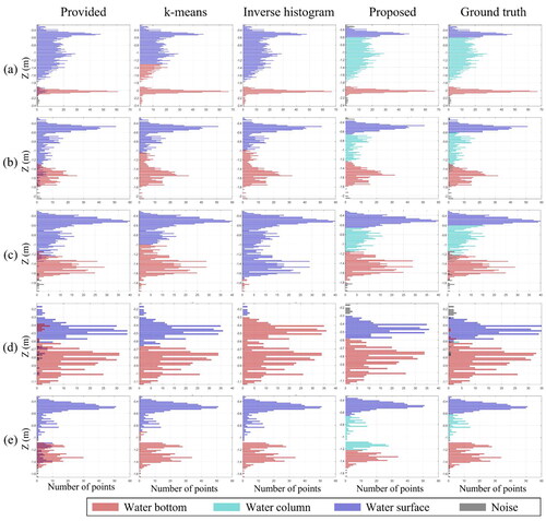
The experimental results in Table 6 and Figure 8 demonstrate that the proposed approach outperforms the other methods in terms of precision, recall, and F1-scores, and visual inspection of the classified water bottom points. Although the provided classification shows the highest precision of 99.896%, it has the lowest F1 score of 95.000% because many water bottom points are not correctly classified (Figure 8a), resulting in a very low recall rate of 90.562%. On the other hand, the k-means tend to over-classify the water bottom (Figure 8b), resulting in a low precision rate of 92.024% and an F1 score of 95.162%. In Figure 8g, it can be seen that the water bottom classified by the k-means includes some unoccupied cells due to the under-classification caused by the noise under the water bottom. The inverse histogram achieved an F1-score of 97.375%. The inverse histogram also tends to under-classify the water bottom, resulting in some unoccupied cells as shown in Figures 8c and 8h, which are often found in very shallow water. The proposed approach achieved the best F1 score (98.944%) and recall (98.649%) rates, also resulting in visually close to the ground truth (Figure 8d). This is because, unlike the other existing methods, the proposed approach enables multi-classification (i.e., water bottom, column, surface, and noise) that helps prevent over or under-classification. However, some under-classification occurred along the near shore area (Figure 8i) because of the incomplete cells containing an insufficient number of points to generate a valid pseudo waveform.

Figure 8. Classified water bottom points of VQ-880G data: (a–e) close-up view of region #1; and (f–j) close-up view of region #2.

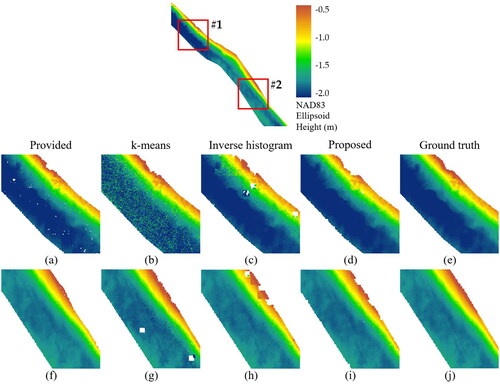
Figure 9 shows some examples of classification results with different depths. Figure 9a depicts an example of a pseudo-waveform with a depth of less than 1.7 m, showing a gap between the water bottom and column. The inverse histogram and proposed methods correctly classified the water bottom, whereas k-means over-classified the water bottom due primarily to the fact that k-means is not suitable for clustering imbalanced data. Figures 9b–9d represent more challenging cases where there are no clear gaps between the water bottom and column, demonstrating that the proposed approach is particularly useful compared with the other existing methods. In addition, the proposed approach can identify the noise present under the water bottom (Figures 9b and 9c) or above the water surface (Figure 9d), which cannot be achieved by the other binary classification methods. Lastly, Figure 9e shows a limitation of the proposed approach where the algorithm failed to fit a single Gaussian curve to the water bottom within a single cell due to uneven topography. This will be investigated in future work.

Figure 9. Examples of classification results by depth and water bottom type: (a) clear separation of the water bottom (depth < 1.7 m); (b,c) unclear separation of the water bottom (depth < 1.3 m); (d) very shallow water (depth < 0.7 m); (e) uneven water bottom (depth < 1 m).

Evaluation with MBES data

Finally, we classified additional data acquired by Seahawk and compared the results with MBES data. Table 7 shows the classification accuracies achieved with the parameter set (χ: 20 m, σ: 4, and τ: 0.3 m) optimized for the Seahawk ABL data. The overall accuracy was determined to be 97.291%, demonstrating that the proposed approach is applicable to other ABL data with parameter adjustment. Unlike the VQ-880-G datasets, we achieved higher accuracy with increased cell and smoothing filter sizes. The large cell size is due primarily to the low point density of the Seahawk datasets, leading the algorithm to have more points within each cell with increased cell size. Likewise, the large smoothing filter size is desirable because it helps prevent over-decomposition caused by the data with low point density. Unlike the above parameters, it was found that the classification is less sensitive to the Z threshold.

Table 7. Optimized parameters and accuracies of the classification result of Seahawk data.

Parameters			Accuracy (%)
Cell size	Filter size	Z threshold	Water bottom			Water surface			Overall accuracy
			Precision	Recall	F1 score	Precision	Recall	F1 score
20 m	4	0.3 m	99.378	98.272	98.822	99.031	97.788	98.406	97.291

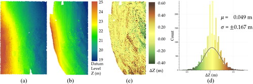
Finally, the water bottom classified by the proposed approach was compared with the MBES data (Figure 10b) acquired in the region. The MBES data, with a point density of 0.98 pt/m², were acquired using RESON Seabet 125 in November 2021. A 4-month time gap exists between the Seahawk ABL and MBES data acquisitions. Since MBES systems generally cannot operate in water depths less than 4 m, the MBES acquired in that region was only measured in about 70% of the entire test site, and a vertical position comparison was performed for this overlapping area. The distances in the Z-direction between the bottom points and the triangular irregular network (TIN) surface of MBES data were calculated (Figure 10c). The results indicate that the water bottom was successfully detected with the mean error and standard deviation of 0.049 ± 0.167 m. Figure 10d shows the histogram of the difference map, showing that the residuals are distributed randomly over the test site.

Figure 10. Error distribution in the Z-direction (ΔZ) of Seahawk data: (a) classified water bottom points; (b) MBES data; (c) the difference map of ΔZ; (d) frequency histogram of ΔZ.

Conclusion

In this study, we proposed a novel approach that uses a custom pseudo-waveform decomposition method for classifying ABL data into different water levels, including the bottom, column, surface, and noise. The experimental results demonstrated that the proposed approach applies to different ABL systems and environments. Compared with the existing methods, the proposed approach is particularly advantageous for the classification of very shallow water (<2 m water depth) containing no clear gaps between different water levels. Further, the proposed approach can detect the noise above the water surface, which occurs due mainly to breaking waves, and noise under the water bottom, which occurs due mainly to signal return delay.

The algorithm assumes that each cell has a sufficient number of points for different water levels, thereby forcing the algorithm to over-classify the water bottom when the water is deep, and returns are barely detectable. This can be improved by comparing the results of nearby cells to detect discontinuity. Future research should also consider the uneven water bottom, which cannot be fitted by a single Gaussian component. This can be solved to some extent by using a small cell size; however, too small a value can lead to high computational costs and sparse points. Alternatively, an object-based clustering that groups the points with similar topographic characteristics can be applied in the pre-processing step. Topographic data, such as elevation or slope, can be generated from the pre-classified water bottom points. Subsequently, the edge detection technique followed by connected component analysis can be applied to split the topographic data. This will produce dense clusters over areas with high undulation while producing coarse, large clusters over flat areas, potentially replacing the grid cells. Lastly, it would be worthwhile to compare the water level classification algorithm developed in this study against other published machine learning algorithms as well as any future approaches.

Acknowledgments

The authors would like to thank NOAA Digital Coast (Office for Coastal Management) for providing Riegl VQ-880G bathymetric LiDAR data.

Disclosure statement

No conflict of interest was reported by the author(s).

Additional information

Funding

This research was supported by Korea Institute of Marine Science and Technology Promotion (KIMST) funded by the Ministry of Oceans and Fisheries [No. 20200623] and Basic Science Research Program through the National Research Foundation of Korea (NRF) funded by the Ministry of Education [No. 2021R1I1A3059263].

Appendix A

 

 

Table A1. Specifications for Riegl VQ-880G system.

Parameter	Specification
Laser wavelength	532 nm (green) 1064 nm (NIR)
Laser pulse width	1.6 ns
Laser beam divergence	0.7–2.0 mrad (green) 0.2 mrad (NIR)
Field of view (FoV)	40°
Pulse repetition rate	550 kHz
Operating flight altitude	600 m
Minimum range (1.5 Secchi depth)	10 m
Main dimensions (L × W × H)	444 × 444 × 695 mm
Weight	65 kg

Table A2. Specifications for Seahawk system.

Parameter	Specification
Laser wavelength	532 nm (green) 1064 nm (NIR)
Laser pulse width	1.7 ns
Laser beam divergence	7 mrad (green) 10.5 mrad (NIR)
Field of view (FoV)	20°
Pulse repetition rate	10 kHz
Operating flight altitude	400 m
Minimum range (1.5 Secchi depth)	10 m
Main dimensions (L × W × H)	442 × 515 × 499 mm
Weight	73 kg

References

- Blue Marble Geographics. 2022. “Global mapper user guide.” Available from https://www.bluemarblegeo.com/knowledgebase/global-mapper-24/GlobalMapper.htm. (accessed October 15, 2022).
- Brock, J.C., and Purkis, S.J. 2009. “The emerging role of Lidar remote sensing in coastal research and resource management.” Journal of Coastal Research, Vol. 10053 (No. SI): pp. 1–5. doi:10.2112/SI53-001.1.
- Chust, G., Grande, M., Galparsoro, I., Uriarte, A., and Borja, Á. 2010. “Capabilities of the bathymetric Hawk Eye LiDAR for coastal habitat mapping: A case study within a Basque estuary.” Estuarine, Coastal and Shelf Science, Vol. 89(No. 3): pp. 200–213. doi:10.1016/j.ecss.2010.07.002.
- CloudCompare. 2015. “CloudCompare user documentation: SOR filter.” Available from https://www.cloudcompare.org/doc/wiki/index.php/SOR_filter (accessed August 1, 2022).
- Daniele, T., Mckean, J.A., Benjankar, R.M., Wright, C.W., Goode, J.R., Chen, Q.W., Reeder, W.J., Carmichael, R.A., and Edmondson, M.R. 2019. “Mapping river bathymetries: Evaluating topobathymetric LiDAR survey.” Earth Surface Processes and Landforms, Vol. 44(No. 2): pp. 507–520. doi:10.1002/esp.4513.
- Guenther, G. C. 1985. Airborne Laser Hydrography: System Design and Performance Factors. Rockville, MD: NOAA Professional Paper Series, National Ocean Service 1, National Oceanic and Atmospheric Administration.
- Guo, K., Xu, W., Liu, Y., He, X., and Tian, Z. 2017. “Gaussian half-wavelength progressive decomposition method for waveform processing of airborne laser bathymetry.” Remote Sensing, Vol. 10(No. 2): pp. 35. doi:10.3390/rs10010035.
- Jung, J., Lee, J., and Parrish, C.E. 2021. “Inverse histogram-based clustering approach to seafloor segmentation from bathymetric LiDAR data.” Remote Sensing, Vol. 13(No. 18): pp. 3665. doi:10.3390/rs13183665.
- Kim, H., Lee, J., Kim, Y., and Wie, G. 2021. “Waveform decomposition of airborne bathymetric LiDAR by estimating potential peaks.” Korean Journal of Remote Sensing, Vol. 37(No. 6–1): pp. 1709–1718. doi:10.7780/kjrs.2021.37.6.1.18.
- Kim, H., Tuell, G.H., Park, J.Y., Brown, E., and We, G. 2019. “Overview of SEAHAWK: A bathymetric LiDAR airborne mapping system for localization in Korea.” Journal of Coastal Research, Vol. 91(No. sp1): pp. 376–380. doi:10.2112/SI91-076.1.
- Kogut, T., and Weistock, M. 2019. “Classifying airborne bathymetry data using the Random Forest algorithm.” Remote Sensing Letters, Vol. 10(No. 9): pp. 874–882. doi:10.1080/2150704X.2019.1629710.
- Kogut, T., Tomczak, A., Słowik, A., and Oberski, T. 2022. “Seabed Modelling by Means of Airborne Laser Bathymetry Data and Imbalanced Learning for Offshore Mapping.” Sensors, Vol. 22(No. 9): pp. 3121. doi:10.3390/s22093121.
- Kumpumäki, T., Ruusuvuori, P., Kangasniemi, V., and Lipping, T. 2015. “Data-driven approach to benthic cover type classification using bathymetric LiDAR waveform analysis.” Remote Sensing, Vol. 7(No. 10): pp. 13390–13409. doi:10.3390/rs71013390.
- Li, X., Liu, C., Wang, Z., Xie, X., Li, D., and Xu, L. 2021. “Airborne LiDAR: State-of-the-art of system design, technology and application.” Measurement Science and Technology, Vol. 32(No. 3): pp. 032002. doi:10.1088/1361-6501/abc867.
- Lloyd, S. 1982. “Least squares quantization in PCM.” IEEE Transactions on Information Theory, Vol. 28(No. 2): pp. 129–137. doi:10.1109/TIT.1982.1056489.
- Lowell, K., and Calder, B. 2021a. “Assessing marginal shallow-water bathymetric information content of lidar sounding attribute data and derived seafloor geomorphometry.” Remote Sensing, Vol. 13(No. 9): pp. 1604. doi:10.3390/rs13091604.
- Lowell, K., and Calder, B. 2021b. “Extracting shallow-water bathymetry from lidar point clouds using pulse attribute data: merging density-based and machine learning approaches.” Marine Geodesy, Vol. 44(No. 4): pp. 259–286. doi:10.1080/01490419.2021.1925790.
- Ma, Y., Zhang, J., Zhang, Z., and Zhang, J.Y. 2019. “Bathymetry retrieval method of LiDAR waveform based on multi-Gaussian functions.” Journal of Coastal Research, Vol. 90(No. sp1): pp. 324–331. doi:10.2112/SI90-041.1.
- Mader, D., Richter, K., Westfeld, P., Weiß, R., and Maas, H.G. 2019. “Detection and extraction of water bottom topography from laser bathymetry data by using full-waveform-stacking techniques.” The International Archives of the Photogrammetry, Remote Sensing and Spatial Information Sciences, Vol. XLII-2/W13: pp. 1053–1059. doi:10.5194/isprs-archives-XLII-2-W13-1053-2019.
- Mallet, C., and Bretar, F. 2009. “Full-waveform topographic lidar: State-of-the-art.” ISPRS Journal of Photogrammetry and Remote Sensing, Vol. 64(No. 1): pp. 1–16. doi:10.1016/j.isprsjprs.2008.09.007.
- Mandlburger, G., Hauer, C., Wieser, M., and Pfeifer, N. 2015. “Topo-bathymetric LiDAR for monitoring river morphodynamics and instream habitats—A case study at the Pielach River.” Remote Sensing, Vol. 7(No. 5): pp. 6160–6195. doi:10.3390/rs70506160.
- Mandlburger, G. 2020. “A review of airborne laser bathymetry for mapping of inland and coastal waters.” Hydrographische Nachrichten, Vol. 116: pp. 6–15. doi:10.23784/HN116-01.
- MathWorks. 2007. “MATLAB documentation: Findpeaks.” Available from https://mathworks.com/help/signal/ref/findpeaks.html (accessed October 1, 2022).
- Muss, J.D., Mladenoff, D.J., and Townsend, P.A. 2011. “A pseudo-waveform technique to assess forest structure using discrete lidar data.” Remote Sensing of Environment, Vol. 115(No. 3): pp. 824–835. doi:10.1016/j.rse.2010.11.008.
- NOAA National Geodetic Survey (NGS). 2022. “2016 NOAA NGS topobathy lidar: Marco Island (FL).” Available from https://www.fisheries.noaa.gov/inport/item/48178 (accessed August 3, 2022).
- Pe’eri, S., and Philpot, W. 2007. “Increasing the existence of very shallow-water LIDAR measurements using the red-channel waveforms.” IEEE Transactions on Geoscience and Remote Sensing, Vol. 45(No. 5): pp. 1217–1223. doi:10.1109/TGRS.2007.894584.
- Schwarz, R., Mandlburger, G., Pfennigbauer, M., and Pfeifer, N. 2019. “Design and evaluation of a full-wave surface and bottom-detection algorithm for LiDAR bathymetry of very shallow waters.” ISPRS journal of Photogrammetry and Remote Sensing, Vol. 150: pp. 1–10. doi:10.1016/j.isprsjprs.2019.02.002.
- Tan, S.H., and Tan, S.B. 2010. “The correct interpretation of confidence intervals.” Proceedings of Singapore Healthcare, Vol. 19(No. 3): pp. 276–278. doi:10.1177/201010581001900316.
- Terrasolid. 2022. “TerraScan user guide.” Available from https://terrasolid.com/guides/tscan.pdf (accessed October 15, 2022).
- Wang, C., Li, Q., Liu, Y., Wu, G., Liu, P., and Ding, X. 2015. “A comparison of waveform processing algorithms for single-wavelength LiDAR bathymetry.” ISPRS Journal of Photogrammetry and Remote Sensing, Vol. 101: pp. 22–35. doi:10.1016/j.isprsjprs.2014.11.005.
- Wedding, L.M., Friedlander, A.M., McGranaghan, M., Yost, R.S., and Monaco, M.E. 2008. “Using bathymetric lidar to define nearshore benthic habitat complexity: Implications for management of reef fish assemblages in Hawaii.” Remote Sensing of Environment, Vol. 112(No. 11): pp. 4159–4165. doi:10.1016/j.rse.2008.01.025.
- Weinstein, M.P., and Heck, K.L. 1979. “Ichthyofauna of seagrass meadows along the Caribbean coast of Panama and in the Gulf of Mexico: Composition, structure and community ecology.” Marine Biology, Vol. 50(No. 2): pp. 97–107. doi:10.1007/BF00397814.
- Xing, S., Wang, D., Xu, Q., Lin, Y., Li, P., Jiao, L., Zhang, X., and Liu, C. 2019. “A depth-adaptive waveform decomposition method for airborne LiDAR bathymetry.” Sensors, Vol. 19(No. 23): pp. 5065. doi:10.3390/s19235065.
- Yang, A., Wu, Z., Yang, F., Su, D., Ma, Y., Zhao, D., and Qi, C. 2020. “Filtering of airborne LiDAR bathymetry based on bidirectional cloth simulation.” ISPRS Journal of Photogrammetry and Remote Sensing, Vol. 163: pp. 49–61. doi:10.1016/j.isprsjprs.2020.03.004.
- Yang, F., Qi, C., Su, D., Ding, S., He, Y., and Ma, Y. 2022. “An airborne LiDAR bathymetric waveform decomposition method in very shallow water: A case study around Yuanzhi Island in the South China Sea.” International Journal of Applied Earth Observation and Geoinformation, Vol. 109: pp. 102788. doi:10.1016/j.jag.2022.102788.
- Zhou, T., and Popescu, S.C. 2017. “Bayesian decomposition of full waveform LiDAR data with uncertainty analysis.” Remote Sensing of Environment, Vol. 200: pp. 43–62. doi:10.1016/j.rse.2017.08.012.