UAV-SfM and Geographic Object-Based Image Analysis for Measuring Multi-Temporal Planimetric and Volumetric Erosion of Arctic Coasts

Abstract

Monitoring and quantifying the rapid changes along Arctic coasts is becoming increasingly important as above average warming in the Arctic is contributing to increasing rates of erosion leading to dramatic impacts on coastal ecosystems and communities. Understanding the impacts of Arctic coastal erosion on the climate system across large coastal scales requires improvements in measurement techniques. We analyzed two coastal sites in Kugmallit Bay (near Tuktoyaktuk, Northwest Territories, Canada), over a one-week and one-year time interval. Using high-resolution imagery from Unoccupied Aerial Vehicles with Structure from Motion (UAV-SfM), we investigated the influence of unique coastal indicator features on reported planimetric and volumetric measurements and explored the use of Geographic Object Based Image Analysis (GEOBIA) to semi-automate the process of coastal feature extraction. We observed temporally dependent differences between coastal feature movements, planimetrically and volumetrically, and object-based feature extraction accuracy was found to be feature dependent. Our research has made methodological improvements to Arctic coastal measurements, particularly at high spatiotemporal scales, which highlights considerations relevant to broad scale Arctic coastal monitoring and quantification.

RÉSUMÉ

La surveillance et la quantification des changements rapides le long des côtes arctiques deviennent de plus en plus importantes, car un réchauffement supérieur à la moyenne dans l’Arctique contribue à l’augmentation des taux d’érosion, ce qui entraîne des répercussions dramatiques sur les écosystèmes et les communautés côtières. Pour comprendre les répercussions de l’érosion côtière en Arctique sur le système climatique à grande échelle, il faut améliorer les techniques de mesure. Nous avons analysé deux sites côtiers dans la baie de Kugmallit (près de Tuktoyaktuk, dans les Territoires du Nord-Ouest, au Canada), sur une période d’une semaine et d’un an. À l’aide d’images haute résolution de drones (UAV-SfM), nous avons étudié l’influence des caractéristiques particulières des côtes sur les mesures planimétriques et volumétriques rapportées et exploré l’utilisation de l’analyse d’images basée sur des objets géographiques (GEOBIA) pour semi-automatiser le processus d’extraction des rives. Nous avons observé des différences temporelles entre les changements des propriétés du rivage, planimétriques et volumétriques, et la précision de l’extraction des caractéristiques basée sur les objets s’est avérée dépendante de la nature des côtes. Notre recherche a apporté des améliorations méthodologiques pour la mesure des rivages de l’Arctique, en particulier à des échelles spatio-temporelles élevées, ce qui met en évidence des considérations pertinentes pour la surveillance et la quantification de l’érosion des côtes de l’Arctique à grande échelle.

Introduction

Arctic coasts are becoming an increasingly important area of research (Fritz et al. 2017) due to the above average warming in the Arctic resulting from climate change (Jorgenson et al. 2006), which is contributing to already high rates of erosion (Lantuit and Pollard 2008; Irrgang et al. 2018; Jones et al. 2009). Further, Arctic coastal erosion leads to the release of stored organic carbon from permafrost and the subsequent transformation into carbon dioxide and methane that impacts carbon cycling and the climate system (Tanski et al. 2019; Ramage et al. 2017). Arctic coasts have been calculated to make up 30–34% of Earth’s coasts of which 65% are composed of more easily eroded unlithified sediments while 35% are more resistant lithified rock (Walker 2005; Lantuit et al. 2012). Average rates of coastal erosion in the Arctic are considered some of the highest in the world and have been reported to average 0.5 m a⁻¹ with 3% exceeding 3 m a⁻¹ of retreat (Lantuit et al. 2012) and some local rates exceeding 20 m a⁻¹ (Günther et al. 2013; Jones et al. 2009; Malenfant et al. 2022; Solomon 2005). Future rates of Arctic coastal erosion are expected to increase due to the lengthening of the open water season and increases in air and water temperatures (Overeem et al. 2011; Stocker et al. 2013; Günther et al. 2015). Declining summer sea-ice cover in the Arctic Ocean, rising sea levels, and increasing storm intensity and frequency combined with increased air temperature are also expected to contribute to increased Arctic coastal erosion by a factor of three (Nielsen et al. 2022). The erosion of permafrost coasts is causing rapid land loss, posing a threat to habitats, archaeologically significant sites, infrastructure, and communities (Mars and Houseknecht 2007). Furthermore, the discharge of organic sediments, which were previously frozen, into nearby water has an impact on marine ecosystems and also contributes to the process of ocean acidification (Semiletov et al. 2016) and threatens the food security of northern residents who rely on marine resources (Ford et al. 2015).

Because of the complex permafrost landscapes found along Arctic coasts, paucity of information regarding short-term coastal dynamics, environmental forcing factors (Jones et al. 2018), and limited spatiotemporal coverage being monitored, there is a significant opportunity to leverage new technologies and approaches in studying the geomorphic character of Arctic coasts and quantifying erosion rates and volumetric changes. Recent developments in Unoccupied Aerial Vehicles with Structure from Motion (UAV-SfM) and the ability of this technology to generate high resolution orthomosaics and digital surface models (DSM) with high temporal flexibility offer new opportunities to study rapid temporal geomorphological changes (James et al. 2019). From this data new techniques can be developed for quantifying coastal change (Berry et al. 2021; Cunliffe et al. 2019; Clark et al. 2021;). Further, the use of Geographic Object Based Image Analysis (GEOBIA) has the potential to assist in the automation of coastal feature extraction, making coastal erosion studies easier and potentially more consistent. In general, GEOBIAs use in coastal geomorphology has been found to be limited (Papakonstantinou et al. 2016; Chen et al. 2018; Hidayat et al. 2018) particularly for investigating Arctic coasts (Clark et al. 2022).

GEOBIA refers to an object-based approach in the analysis of Earth observation remote sensing imagery with the goal of emulating human interpretation of remotely sensed imagery through the use of image segmentation and classification based on image-objects (Castilla and Hay 2008). Image segmentation provides the basic units (primitives) of GEOBIA (Hay and Castilla 2008). Segments contain spectral information, like pixels, but also include measures of median values, minimum and maximum values, variance, and texture but of greater benefit is the addition of spatial information like distances, neighborhood, topologies, and expert knowledge (Blaschke 2010). Through the creation of rule sets, classification, and feature extraction can be repeated, creating a systematic approach that can be applied across studies or through time.

Our research leverages UAV-SfM datasets over three time steps at two coastal sites in the Western Canadian Arctic near the hamlet of Tuktoyaktuk, NT to quantify geomorphic changes occurring over a one-week period capturing a substantial storm event and a roughly one-year period capturing seasonal changes. Further, two site-specific GEOBIA rule sets were developed and applied to all datasets to create a coastal classification and subsequently extract important linear coastal features. Specifically, our objectives were to: (1) quantify and compare the weekly and seasonal planimetric and volumetric changes at our two studies, (2) extract linear coastal indicator features (waterline, cliff toe, cliff edge) using GEOBIA rule sets and compare the quality against manually delineated features. It was hypothesized that GEOBIA will improve coastal classification, however, the local geomorphology may contribute to differences in planimetric and volumetric change between study sites despite the relatively close proximity and similar exposure. In addition, we hypothesized there may be a feature-specific dependency on the accuracy of GEOBIA extracted coastal features relative to our manually delineated features.

Study area

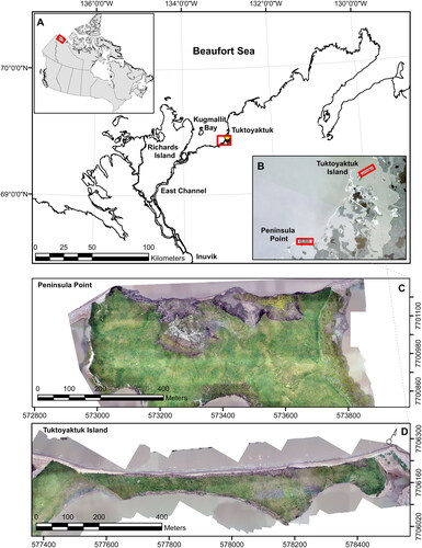
Two coastal sites located in the Beaufort Sea of the Western Canadian Arctic (Figure 1) in the Northwest Territories were investigated. This region has experienced significant coastal erosion (Dallimore et al. 1996; Manson et al. 2005; Forbes et al. 2014) and the close proximity of the study sites to the Hamlet of Tuktoyaktuk lend to favorable field logistics and a rich history of research (Moorman et al. 1998; Mackay and Burn 2002; Solomon 2005; Whalen et al. 2022). Tuktoyaktuk Island (69°27′10.76″N, 133° 0′56.59″W) (Figure 1D) is located <1 km to the east of the Hamlet of Tuktoyaktuk and provides protection from incident waves for the local harbor. Peninsula Point (69°24′31.23″N, 133° 7′48.38″W) (Figure 1C) is located 5 km south west of the Hamlet of Tuktoyaktuk. Tide gauge records at Tuktoyaktuk indicate a tidal range of ±30 cm with local chart datum (CD) ∼0.45 m below mean sea level (MSL) (Kim et al. 2021). A one in 100 year return period of a storm surge at Tuktoyaktuk is considered to be at least 2.10 m (Kim et al. 2021). The mean annual temperature recorded at Tuktoyaktuk, NT between 1981 and 2010 was −10.1 °C with average daily temperatures of −26.6 and 11.0 °C in January and July, respectively. The average annual temperate during the open water season has increased by 3 °C (Berry et al. 2021). Meanwhile, the annual precipitation is 160.7 mm with 103.1 mm of it being in the form of snowfall with water equivalence (Environment and Climate Change 2020).

Figure 1. (A) Map of the study area found in the western Canadian Arctic in the southern Beaufort Sea near the hamlet of Tuktoyaktuk, NT. (B) Relative location of the two study sites. (C) Peninsula Point study site. Shown is the extent of a UAV survey in true-colourmosaic from 2018 (D1). The Peninsula Point study site is a polycyclic retrogressive thaw slump coastal environment with actively flowing thaw slumps and exposed massive ice in the headwall. (D) Tuktoyaktuk Island study side. Shown is the extent of a UAV survey in true-colourmosaic from 2018 (D1). Tuktoyaktuk Island is a coastal cliff environment with limited exposed massive ice and a small inactive thaw slump near the center of the survey area. Boundary polygons from the Atlas of Canada, National Scale Data 1:1,000,000 retrieved from Natural Resources Canada through the Open Government License. Base map data on inset map B retrieved from Planet Labs Inc. Map created using ArcMap 10.6. Permission is not required for use of this map.

We studied a roughly 1 km stretch at Tuktoyaktuk Island, which has a north-north western exposure and is dominated by 10 m high sand and silty cliffs (Whalen et al. 2022). Peninsula Point has a northern exposure, of which we studied the entire northern coastal stretch (650 m). Peninsula Point is dominated by a coastal polycyclic retrogressive thaw slump (RTS) environment of clay-rich sediment with an average headwall height of 5–10 m, which can contain up to 10 m high sections of exposed massive ice in any given year and ice thickness up to 20 m but typically between 10 and 16 m (Moorman et al. 1998). Permafrost on the Tukyotaktuk Peninsula is widespread ranging from 200 to 500 m in thickness (Judge et al. 1987) with a volumetric ground ice content of 29% (Lantuit et al. 2012). Permafrost thaw and melting ice cause widespread rapid coastal changes at these study sites. The region is typically ice-free from late June to October but changes in the Arctic sea ice regime have resulted in longer ice-free seasons (Meier et al. 2014; Lindsay and Schweiger 2015), causing increased wave activity due to a lengthening of open-water fetch. The shallow nearshore profile in the region contributes to dampening wave action along the coasts, which are dominated by prevailing northwest winds, however, elevated water levels during storm surge events allow waves to interact with coastal sediments (Dallimore et al. 1996; Harper 1990) leading to coastal modification. Storm surges above chart datum (CD) have reached 2.95 m and regularly exceed 1 m (Kim et al. 2021; Solomon et al. 1994) contributing to coastal erosion rates exceeding 5 m a⁻¹ (Forbes and Frobel 1985; Mackay 1986; Harper 1990; Hill et al. 1991) despite a relatively short open water season.

Materials and methods

UAV data collection and processing

Unoccupied aerial vehicle (UAV) data were collected on three dates at each of the study sites. At Tuktoyaktuk Island, the three dates of data collection were August 9, 2018, August 18, 2018, and June 20, 2019. The dates of data collection at Peninsula Point were August 11, 2018, August 19, 2018, and June 18, 2019. Herein, these datasets will be referred to as D1, D2, and D3 at each respective study site. There is roughly a one-week period between D1 and D2 at which point a storm surge event from the northwest with wave heights of ∼1 m over a roughly 7-h timeframe occurred. The roughly 300 days between D2 and D3 represent the conditions from mid to late summer to early summer shortly after the ice breakup in the following year. Over this timeframe, there were fewer than three months of ice-free conditions found along the coastal sites.

Due to equipment availability over multiple field campaigns, several UAV platforms were utilized for data collection. All 2018 datasets were collected using a DJI M210 with X4S sensor, which was equipped with a 1″ 20 megapixel RGB sensor with 8.8 mm focal length (35 mm equivalent) and leaf shutter. Flight planning and mission execution was conducted using the Pix4D Capture mobile app. At Peninsula Point, D3 was gathered utilizing a senseFly eBee X fixed-wing system that had the RTK feature enabled. The onboard camera employed for this task was a senseFly S.O.D.A 3D that comes with a 1″ 20-megapixel RGB sensor. Additionally, the camera includes a global shutter and has a focal length of 10.6 mm. Flight planning and mission execution was conducted with senseFly eMotion 3.7 software. D3 at Tuktoyaktuk Island was collected using a DJI Phantom 4 RTK equipped with a 1″ 20-megapixel RGB sensor with 8.8 mm focal length (35 mm equivalent) and mechanical shutter.

A Hemisphere S321 antenna was established as a base station over an unknown location found within the study area for D1 with associated horizontal (X, Y) and vertical (Z) instrument accuracies of (0.009, 0.016, 0.031) m at Tuktoyaktuk Island and (0.008, 0.015, 0.031) m at Peninsula Point. A second Hemisphere S321 antenna communicated through RTK with the base station to accurately measure the locations of ground control points (GCPs) and independent check points that were distributed throughout the survey area. To achieve a more precise position for the GNSS data collected by the base station, the Canadian Spatial Reference System (CSRS) Precise Point Positioning (PPP) tool, offered by Natural Resources Canada’s Canadian Geodetic Survey, was employed for post-processing. During the data collection, the base station operated continuously for over 5 h. To utilize the CSRS PPP tool, the input required was the RINEX file generated by the base station, which improved the positional accuracy of the base station, and an offset was applied to the original GCP horizontal coordinates. Imagery from all datasets were processed using Pix4Dmapper 4.4.12 commercial software on a Windows 10 Enterprise 64-bit system with i7-8700K CPU @3.70 GHz, 32 GB RAM, and NVIDIA GeForce RTX 2080 GPU. Flight details and processing specifics are summarized in Table 1.

Table 1. UAV-SfM data collection and processing specifications.

	Tuktoyaktuk Island			Peninsula Point
Date	2018-08-09 (D1)	2018-08-18 (D2)	2019-06-20 (D3)	2018-08-11 (D1)	2018-08-19 (D2)	2019-06-18 (D3)
Platform	DJI M210	DJI M210	DJI Phantom 4 RTK	DJI M210	DJI M210	senseFly eBee X
Sensor
Flying height (AGL)	70 m	70 m	70 m	70 m	70 m	90 m
Overlap (%) (side lap/end lap)	70/80	70/80	70/80	70/80	70/80	70/80
Number of images	674/699 calibrated	867/923 calibrated	1247/1348 calibrated	899/942 calibrated	306/310 calibrated	1084/1159 calibrated
GSD	2.04 cm	2.11 cm	2.38 cm	1.93 cm	2.28 cm	3.28 cm
Number of GCP	5	0	0	6	0	0
Manual tie points	0	7	7	0	5	5
Number of check points	18	14	14	18	10	10
Instrument accuracy	(0.009, 0.016, 0.031) m	NA	NA	(0.008, 0.015, 0.031) m	NA	NA
Processing software	Pix4D 4.4.12	Pix4D 4.4.12	Pix4D 4.4.12	Pix4D 4.4.12	Pix4D 4.4.12	Pix4D 4.4.12
MAE (X, Y, Z)	(0.04, 0.1, 0.29) m	(0.03, 0.02, 0.13) m	(0.03, 0.03, 0.15) m	(0.02, 0.01, 0.05) m	(0.02, 0.06, 0.06) m	(0.07, 0.09, 0.14) m
Conditions	Overcast, 20 km/h wind	Mix of sun and cloud, 20 km/h wind	Overcast, 20 km/h wind	Overcast, 20 km/h wind	Overcast, 20 km/h wind	Overcast, 20 km/h wind

Four different UAV platforms and sensors were used. Image acquisition was kept to a consistent overlap and flying height above ground level. The ground sampling distance varied between surveys, but all data was down sampled to a common resolution of 0.1 m. The number of check points varied between surveys and D2 and D3 were co-registered to D1 at both study sites. Note that some of the images of water around the outside of the study area could not be calibrated due to a lack of identifiable tie-points. The total and number of images calibrated are shown below.

D2 and D3 were co-registered to D1 at each study site due to insufficient raw GPS data coverage in some of these datasets. This approach was chosen to ensure dataset consistency and limit georeferencing errors. D1 were processed using five and six GCP while reserving 13 and 12 as independent check points at Tuktoyaktuk Island and Peninsula Point, respectively. Further, common manual tie points were identified in all datasets, and a subset was used for georeferencing during D2 and D3 processing. In total, 14 manual tie points were identified at Tuktoyaktuk Island and 10 manual tie points were identified at Peninsula Point. At Tuktoyaktuk Island, seven were used for georeferencing with the remaining seven being used as independent check points. At Peninsula Point, five were used for georeferencing with the remaining five used as independent check points. Mean absolute error (MAE) calculations using GPS points and manual tie points were employed to evaluate the horizontal and vertical accuracy of the resulting datasets (James et al. 2019) and are reported in Table 2. Finally, all datasets were down sampled to a common 0.1 m resolution using a bilinear resampling technique in ArcMap 10.6. Through internal testing, this imagine resolution was found to strike the right balance between image detail and processing efficiency, which prevented system crashing when working with GEOBIA segmentations.

Table 2. Mean absolute error (MAE) (m) and standard deviation (SD) (m) for all data sets at the Peninsula Point and Tuktoyaktuk Island study sites reported for each direction.

	MAEx	MAEy	MAEz	SDx	SDy	SDz
Tuktoyaktuk Island
D1	0.04	0.10	0.29	0.08	0.15	0.31
D2	0.03	0.02	0.13	0.04	0.03	0.16
D3	0.03	0.03	0.15	0.04	0.04	0.21
Peninsula Point
D1	0.02	0.01	0.05	0.06	0.02	0.05
D2	0.02	0.06	0.06	0.02	0.06	0.05
D3	0.07	0.09	0.14	0.07	0.12	0.11

Independent check points were evaluated against GPS points for resulting MAE of each dataset.

Planimetric and volumetric measurements

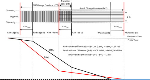
Coastal indicator features were extracted using manual identification on 0.1 m resolution datasets. The identified coastal features at the Peninsula Point and Tuktoyaktuk Island study sites were the waterline, cliff toe, and cliff edge (Figure 2). Features were identified on three datasets at respective study sites (D1, D2, and D3) and were used to quantify the planimetric movement over a weekly and seasonal time step. Planimetric movements in coastal features were quantified using the USGS Digital Shoreline Analysis System (DSAS version 5) extension for ArcGIS (Thieler et al. 2009) by casting a set of transects, from a baseline feature, which intersects the coastal line features. For a given feature, the distance between intersecting points along a transect represents the net shoreline movement (NSM) where the error is represented by the standard deviation. The NSM movement for D1–D2 and D1–D3 were calculated using DSAS with D2–D3 calculated by subtracting the previous two values. A common set of transects was used at each study site, which enabled the direct comparison between coastal feature movements along each transect (Figure 2).

Figure 2. Coastal measurement schematic shown in planimetric and profile view. Three coastal features (waterline, cliff toe, and cliff edge) are used to measure net shoreline movements (NSM) between temporally spaced datasets. Coastal features from both time intervals are used to create cliff and beach envelopes used in volume change calculations. The volume change found within the transition zone, the overlap in cliff and beach envelopes, are subtracted from the total volume change to account for double counting of this area. NSM are calculated along 2 m spaced transects, oriented roughly perpendicular to coastline orientation. Change envelopes are bounded laterally by adjacent transects.

Total uncertainty for a given feature was calculated using Equation (1)(1) $$U=E_G+\mathrm{ }{E}_P+\mathrm{ }{E}_D$$(1) where E_G is the georeferencing error, E_P is the pixel error, and E_D is the digitizing error (Irrgang et al. 2018; Radosavljevic et al. 2016; Río and Gracia 2013; Cunliffe et al. 2019). E_G was dataset specific and calculated using check points and represented by the mean absolute error (MAE). E_P was common among all datasets with a value of 0.1 m and E_D was estimated as three times the pixel error. An additional source of potential error not accounted for here but could contribute to digitizing error is related to cliff overhangs where the apparent cliff edge position is misclassified due to the difficulty of identifying overhang features from 2D imagery. The interpreter must decide whether to digitize the overhang or estimate the cliff edge based on the presence of land separation at the cliff edge. (1) $$U=E_G+\mathrm{ }{E}_P+\mathrm{ }{E}_D$$(1)

Volume change quantification was achieved by creating a DEM of difference (DoD) surface where the later DSM was subtracted from the early DSM (Figure 2) using the Minus geoprocessing tool in ArcMap 10.6. Cliff and beach change envelopes were created from 2D boundary segments for corresponding DoD. Beach change envelope segments were bounded by the seaward waterline and the landward cliff toe features for a given time interval. Further, envelope segments were bounded to the east and west by adjacent transects. Cliff change envelope segments were bounded by the seaward cliff toe and the landward cliff edge feature for a given time interval, and adjacent transects. The relative surface volume difference (DoD) was calculated for each envelope segment for each time step (D1–D2, D2–D3, and D1–D3) using the Zonal Statistics as Table tool in ArcMap 10.6. The resulting sum of pixel values for each segment was multiplied by the cell size (0.1 × 0.1 m) returning the relative volume difference for individual change envelope segments. The transition zone (Figure 2) represents the overlap of the cliff and beach envelopes due to the movement of the cliff toe feature, which is a common boundary feature between envelopes. The volume of the transition zone was calculated and subtracted from the total volume change to account for the overlap. A spatial join was made to the corresponding change envelope feature and the transect layer for each set of segments, which enabled the direct comparison between time steps and to NSM measurements. Because the segments were two meters wide due to the transect spacing creating the segments, volume change quantifications were divided by the segment width and presented with units of volume per meter of coastline (m³/m).

GEOBIA feature extraction

Geographic Object Based Image Analysis, or GEOBIA, was used to classify multi-temporal datasets into vegetation, cliff, beach, and water classes. The boundaries between classes represent extracted coastal indicator features of interest; cliff edge, cliff toe, and waterline. A fourth feature was identified at Peninsula Point as the headwall edge of the polycyclic RTS, over 100 m landward of the waterline feature, but was not elected to be used in analysis due to poor data coverage in D2. Trimble’s eCognition Developer 9.5 software was used to develop a single rule set for each study site that was applied to respective dates of data collection. Rule sets were used to segment, classify, merge, and export geo-objects as shapefiles and subsequently imported into ESRI’s ArcMap 10.6 (Figure 3). Rule sets varied slightly between study sites utilizing site specific thresholds for slope and layer arithmetics at Tuktoyaktuk Island (Equation 2(2) $$\mathit{VARI}=\mathrm{ }\frac{\mathit{Green}-\mathit{Red}}{\mathit{Green}+\mathit{Red}-\mathit{Blue}}$$(2) ). The Visible Atmospherically Resistant Index (VARI) (Gitelson et al. 2002) used at Tuktoyaktuk Island was found to provide good discrimination of vegetation using only the available red, blue, and green bands as compared to other indices. (2) $$\mathit{VARI}=\mathrm{ }\frac{\mathit{Green}-\mathit{Red}}{\mathit{Green}+\mathit{Red}-\mathit{Blue}}$$(2)

Figure 3. GEOBIA rule sets developed using eCognition Developer 9.5 software for the Peninsula Point and Tuktoyaktuk Island study sites. Rule sets utilized multiresolution segmentation, assign class, and merge to create geo-objects. Geo-objects were export as shapefiles and processed in ArcMap 10.6 to create individual line features.

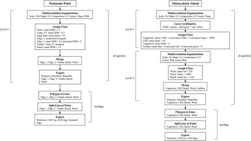
Shapefiles exported from eCognition were brought into ArcMap as polygons and processed into lines to represent the coastal features. This process was done by first using the Polygon to Polylines tool. A new point file was created, and points were placed at the western and eastern extents of the polyline and by using the Split Line at Points tool a line representing the coastal feature associated with that polyline was created. This process was completed for each feature and a new feature class was created from the split line. The accuracy of the coastal feature lines created using a GEOBIA workflow were evaluated against independently extracted coastal features using manual delineation. The USGS Digital Shoreline Analysis System (DSAS) (Thieler et al. 2009) was repurposed to calculate the difference between GEOBIA features and manually digitized features along a given transect. Transects were cast from a baseline to intersect the features at an approximately perpendicular angle with a chosen 2 m transect spacing.

Results

Planimetric and volumetric change measurements

The three time steps of data collection (D1, D2, and D3) are separated by 9 days between D1 and D2 over which time a significant northwestern storm event occurred and 306 (∼90 ice free) days between D2 and D3 at Tuktoyaktuk Island. At Peninsula Point, D1 and D2 are separated by 8 days and contained the same NW storm. The timespan between D2 and D3 at Peninsula Point was 303 (∼90 ice free) days. As a result, we present our results as a net shoreline movement rather than an endpoint rate of change. Summary results for net movement between time steps are presented in Table 3. Positive values indicate a seaward movement and negative values indicate a landward movement (erosion) over time. Furthermore, volumetric change (m³/m) is presented in Table 3 where positive values indicate a volume loss and negative values indicate volume gain. Using the associated uncertainty for a given dataset from Equation (1)(1) $$U=E_G+\mathrm{ }{E}_P+\mathrm{ }{E}_D$$(1) , the uncertainty of planimetric measurements at Tuktotaktuk Island was estimated as ±0.9 and ±0.8 m at Peninsula Point.

Table 3. Average planimetric and volumetric changes calculated between each time step at both study sites.

	Planimetric NSM (m)			Volumetric change (m^3/m)
	Waterline	Cliff toe	Cliff edge	Beach	Cliff
Tuktoyaktuk Island
D1–D2	2.78	−1.33	0.1	4.57	4.17
D2–D3	5.56	0.41	−0.57	2.16	4.6
D1–D3	8.35	−0.92	−0.47	9.05	8.8
Peninsula Point
D1–D2	1.63	−2.17	−0.66	1.65	4.53
D2–D3	−0.53	−1.0	−1.97	2.47	13.71
D1–D3	1.1	−3.17	−2.63	4.23	18.95

The waterline tended to move seaward (positive, accretion) whereas the cliff toe and edge features tended to move landward (negative, erosion). Positive volume change indicates volume loss.

Tuktoyaktuk Island

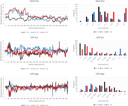
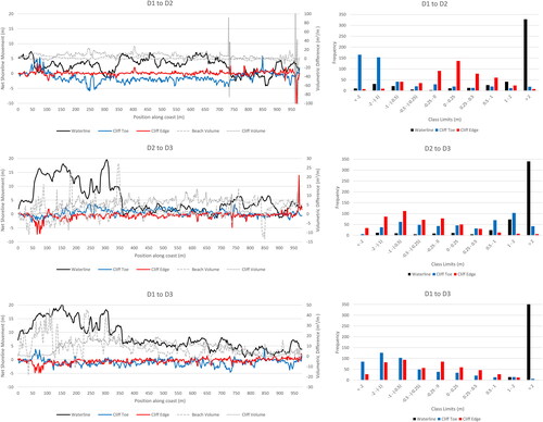
With a 2 m transect spacing along the roughly 900 m coastline at Tuktoyaktuk Island, the average waterline movement between D1 and D2 was calculated to be 2.78 m (seaward movement), with the cliff toe feature changing by an average of −1.33 m (landward movement), and the cliff edge resulting in an average of 0.1 m. The second time step (D2–D3), showed the waterline progressing seaward a further 5.56 m on average, with the cliff toe moving seaward at an average of 0.41 m, whereas the cliff edge retreated landward at an average of 0.57 m. Over the entire timespan (D1–D3), the average waterline position moved seaward by 8.35 m, the cliff toe retreated landward by 0.92 m, and the cliff edge position moved landward with an average of 0.47 m. Individual measurements along each transect are shown in Figure 4 along with measurement frequency occurrence. The entire timespan (D1–D3) is influence by its component parts (i.e., D1–D2 and D2–D3) and will follow the most dominate change as shown in Figure 4 where large movement of the waterline occurred over the first 200 transects of measurement moving west to east during the D2–D3 time step. Further, along the study area, change in the waterline is dominated by the D1–D2 time step for 150 transect measurements. The change in the cliff toe feature was majority erosion during the first time step (D1–D2) and majority accretion, or seaward movement, during the second time step (D2–D3) resulting in the average change over the entire time span (D1–D3) in red. Conversely, the cliff edge feature experienced the most landward movement, or erosion, during the second time step (D2–D3) but was relatively stable during the first time step (D1–D2) outside some anomalous areas.

Figure 4. Net shoreline movement (NSM) for each coastal feature along the Tuktoyaktuk Island coastal site by time interval moving from west to east. Included are frequency occurrence graphs showing which class ranges are most common depending on the feature and time interval. Note the class range difference of the waterline feature to the cliff toe and edge class ranges. Negative values indicate landward movement (erosion) and positive value indicate seaward movement (accretion). NSM is feature and temporarily dependent.

Summary volumetric change analysis results based on transect spacing presented in Table 3 show an average loss in beach volume between D1 and D2 of 4.57 m³/m, a loss of 2.16 m³/m between D2 and D3, and a total average volumetric loss of 9.05 m³/m over the dates of data collection. The volume loss of the cliff that occurred between D1 and D2 was 4.17 m³/m. Similar average volume loss occurred between D2 and D3 at 4.6 m³/m. The total average volume loss was calculated to be 8.8 m³/m. Over the entire stretch of analyzed coast between D1 and D3, there was a total loss in beach volume of 8853 m³ and cliff volume of 8609 m³. When accounting for the transition zone volume, the total volume loss over the seasonal time step was 16,518 m³. Direct comparisons between feature measurements by time step are shown in Figure 5. During the first time step (D1–D2), there was considerable cliff volume change and relatively low beach volume change along the majority of the study site. Along the majority of the study site, we saw stability in the cliff edge position but consistent erosion of the cliff toe. The waterline tended to move seaward but was somewhat more variable along the study site. Again over the second time step, the cliff volume change was more pronounced than the beach volume change, although cliff volume change was more variable compared to the first time step. Cliff and beach volume loss dominated along the study site over the entire time span. The overall magnitude of the planimetric movement of the cliff toe and edge were considerably less than the waterline movement, which exceeded 10 m of seaward movement in many cases.

Figure 5. Direct comparison of net shoreline movement to volumetric measurements along the Tuktoyaktuk Island coastal site, moving west to east, by time interval. NSM are calculated along shore perpendicular transects and volume change is calculated from a DEM of difference (DoD) based on cliff and beach change envelopes. Planimetric erosion is denoted by negative values while volume loss is denoted by positive values. Over short time scales, the change in planimetric movement of coastal features differs while over longer time scales, coastal features tend to converge. Similarly, volumetric change between the cliff and beach becomes more uniform over longer time scales.

Peninsula Point

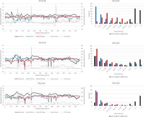
Using 2 m transect spacing over the roughly 650 m coastline at Peninsula Point resulted in an average seaward movement of the waterline feature between D1 and D2 of 1.63 m. Between D2 and D3, the waterline position moved landward at an average of 0.53 m corresponding to an average seaward movement of the waterline position from D1 to D3 of 1.10 m. The cliff toe position retreated landward (erosion) during both time steps for a total average landward retreat of 3.17 m. The cliff toe position moved landward by an average of 2.17 m during the first time step (D1–D2) and 1.0 m during the second time step (D2–D3). Similarly, the cliff edge retreated landward, on average, during both time steps corresponding to 0.66 m between D1 and D2 and 1.97 m from D2 to D3. The total average landward retreat of the cliff edge was calculated to be 2.63 m. Individual measurements along each transect are shown in Figure 6 along with measurement frequency occurrence.

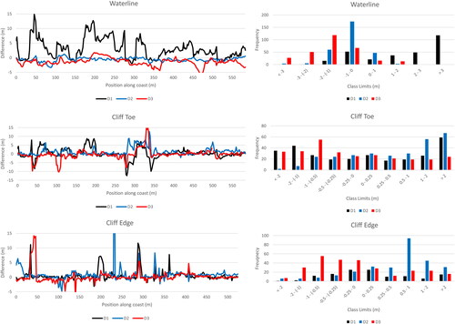
Figure 6. Net shoreline movement (NSM) for each coastal feature along the Peninsula Point coastal site by time interval moving from west to east. Included are frequency occurrence graphs showing which class ranges are most common depending on the feature and time interval. Note the class range difference of the waterline feature to the cliff toe and edge class ranges. Negative values indicate landward movement (erosion) and positive value indicate seaward movement (accretion). NSM is feature and temporarily dependent. The waterline position varied between landward and seaward movements, the cliff toe primarily moved landward but moved seaward in some cases depending on time interval, while the cliff edge moved landward in almost all cases.

The position of the waterline during the first (D1–D2) and second (D2–D3) time steps are approximately mirrored where when the waterline moves seaward during the first time step it is followed by a landward movement, or reduced seaward movement, during the second time step. Overall, the waterline moved seaward except at the western and eastern boundaries of the study site. The cliff toe position at Peninsula Point moved landward along the majority of the study site outside a few anomalous areas during the second time step where the cliff toe position move seaward. There is no discernable difference between the cliff toe movements during the first of second time steps. Conversely, the cliff edge position was relatively stable over the first time step while experiencing consistent landward movement during the second time step.

We used the same method as the Tuktoyaktuk Island study site to calculate the volumetric change using beach and cliff change envelopes. From this, we found the beach lost an average of 1.65 m³/m between D1 and D2 and a further loss of 2.47 m³/m between D2 and D3. In total, an average of 4.23 m³/m of beach volume loss occurred over the study timeframe. Further, the cliff experienced an average volume loss of 18.95 m³/m over the study timeframe, of which 4.53 m³/m of loss occurred from D1 to D2 and 13.7 m³/m of volume loss occurred between D2 and D3. Over the entire stretch of analyzed coast, there was a total of 2693 m³ beach volume loss and 12,050 m³ of cliff volume loss. Accounting for the transition zone, a total loss of 12,920 m³ occur at Peninsula Point between D1 and D3. Direct comparisons between feature measurements by time step are shown in Figure 7. During the first time step, there was cliff volume loss and beach volume gain along the majority of measurement units. The cliff edge was relatively stable with instances of landward movement, however, the cliff toe experienced small to large landward movement along all measurements. Conversely, the waterline moved seaward in all cases. During the seasonal time step, the waterline continued to move seaward in the majority of cases but experienced some landward movement. The beach volume change during the seasonal time step was relatively stable with a net loss compared to the cliff volume change, which was considerably variable with areas with large loss in volume. The cliff volume change during the seasonal time step dominated over the entire time span contributing to substantial volume loss along the study site. By comparison, the beach volume was relatively stable along the study site over the entire time span while the cliff volume loss was more variable with very high loss in some locations.

Figure 7. Direct comparison of net shoreline movement to volumetric measurements along the Peninsula Point coastal site, moving west to east, by time interval. NSM are calculated along shore perpendicular transects and volume change is calculated from a DEM of difference (DoD) based on cliff and beach change envelopes. Planimetric erosion is denoted by negative values while volume loss is denoted by positive values. The cliff toe (slump lobe) and cliff edge (headwall) were spatially distant, but both tended to move landward at a similar magnitude and during each time interval. Volume change tended to be dominated by cliff volume change in part due to the larger change envelope and relatively small beach area at this site.

GEOBIA feature extraction

A sample GEOBIA classification and manual interpretation of coastal indicator features for D1 at both studies sites show the relative differences between extraction methods where classification boundaries were used as linear coastal features (Figure 8). Mean differences between coastal features extracted using GEOBIA and manual digitization are visualized in Figure 9 for Tuktoyaktuk Island and Figure 10 for Peninsula Point.

Figure 8. Study sites Tuktoyaktuk Island (A) and Peninsula Point (D) shown in true colour orthomosaic. Classification results derived from GEOBIA rulesets at Tuktoyaktuk Island (B) and Peninsula Point (E) showing enlarged spatial extents represented in panels C and F. Classified images shown in panels B and E used to derived coastal features at Tuktoyaktuk Island (C) and Peninsula Point (F) based on the boundary lines between classes. Extracted line features follow the classification boundaries more closely at Tuktoyaktuk Island than Peninsula Point where the coastal environment is more complex. Note that the irregular illumination in A and D caused by variable lighting during data collection was mitigated by utilizing an object-based approach that leverages homogeneous region building.

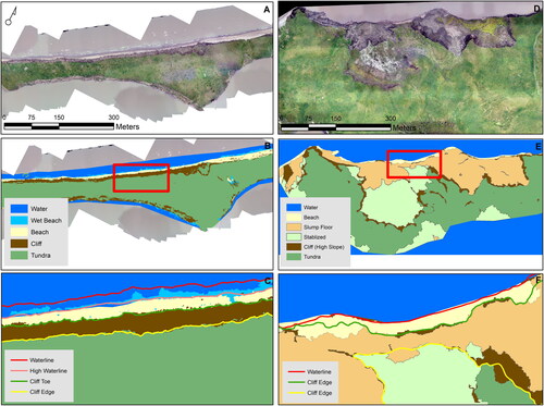
Figure 9. GEOBIA feature extraction accuracy for each coastal feature according to time interval along the Tuktoyaktuk Island coastal site. Each line represents the difference between the GEOBIA extracted coastal feature and the manually identified feature for a given dataset. Positive values indicate the GEOBIA feature was seaward of the manually identified feature. Note the different scales between features indicating the waterline was extracted with reduced accuracy. Frequency occurrence graphs help identify accuracy in GEOBIA feature detection relative to a set of class ranges. Note the difference in frequency scale and class ranges of the waterline feature.

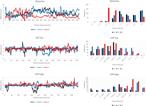
Figure 10. GEOBIA feature extraction accuracy for each coastal feature according to time interval along the Peninsula Point coastal site. Each line represents the difference between the GEOBIA extracted coastal feature and the manually identified feature for a given dataset. Positive values indicate the GEOBIA feature was seaward of the manually identified feature. Note the different scales between features indicating the waterline was extracted with reduced accuracy. Frequency occurrence graphs help identify accuracy in GEOBIA feature detection relative to a set of class ranges. Note the difference in frequency scale and class ranges of the waterline feature.

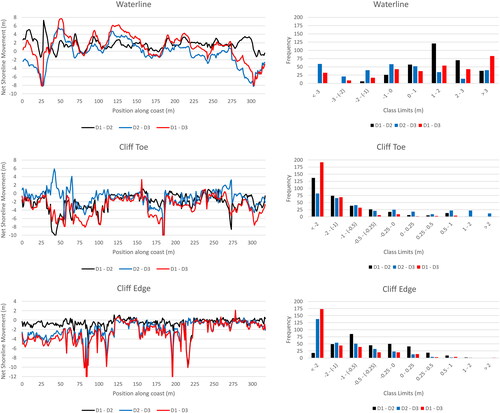
Using Equation (1)(1) $$U=E_G+\mathrm{ }{E}_P+\mathrm{ }{E}_D$$(1) , total uncertainties associated with manually digitized features are 0.52 m at Tuktoyaktuk Island and 0.46 m at Peninsula Point study sites. For the purposes of comparison between feature extraction methods, manually digitized features are assumed to be the “true” features and were carefully assessed using the same interpretation and interpreter in succession. Manual features were subtracted from GEOBIA features meaning that a positive value indicates that the position of the manual feature was seaward from the GEOBIA feature whereas a negative value indicates the manual feature was landward of the GEOBIA feature. There is considerable variability depending on dataset and coastal feature (Table 4). At the Tuktoyaktuk Island study site, the position of the waterline had an average difference of 3.9 m on D1, 3.8 m on D2, and 2.0 m on D3, whereas at the Peninsula Point study site, the position of the waterline had an average difference of 3.0 m on D1, −0.59 m on D2, and −1.42 m on D3. There was a seaward bias of the cliff toe GEOBIA features at Tuktoyaktuk Island for all datasets; −0.64 m for D1, −0.61 m for D2, and −0.32 m for D3. The GEOBIA cliff toe features at Peninsula Point were biased landward for D1 (0.24 m) and D2 (1.29 m) but biased, on average, seaward of the manually digitized feature on D3 (−0.27 m). Identification of the cliff edge coastal feature produced similar absolute values between study sites where D1 corresponded to an average difference of −0.4 m at Tuktoyaktuk Island and 0.64 m at Peninsula Point, D2 corresponding to −0.61 m at Tuktoyaktuk Island and 1.51 m at Peninsula Point, and D3 corresponding to 0.93 m at Tuktoyaktuk Island and 0.14 m at Peninsula Point.

Table 4. GEOBIA extracted coastal features compared to manually digitized features.

	Waterline (m)	Cliff toe (m)	Cliff edge (m)
Tuktoyaktuk Island
D1	3.89	−0.64	−0.41
D2	3.85	−0.61	−0.61
D3	2.03	−0.32	0.93
Peninsula Point
D1	3.03	0.24	0.63
D2	−0.59	1.3	1.51
D3	−1.43	−0.27	0.14

A positive value indicates the GEOBIA feature was measured landward of the manual feature and a negative value indicates the GEOBIA feature was measured seaward of the manual feature.

There was a considerable difference in the ability of the GEOBIA rulesets developed to identify the waterline compared to the cliff toe and edge features at Tuktoyaktuk Island compared to manually identified features (Figure 9). The GEOBIA waterlines for D1 and D2 produced similar results but were approximately inversed to D3 where when there was higher agreement in D3 there was lower agreement in D1 and D2 and vice versa. The difference can likely be attributed to the spectral difference between the datasets where D1 and D2 were captured a week apart in August and D3 was captured in June where there was a more uniformly brown color to the scene. There is no visibly distinguishable difference between datasets in the extraction of coastal cliff edge and toe positions, which were primarily identified using the slope of the scene derived from the DSMs, limiting the temporal reliance. There was similar consistency at Peninsula Point across datasets in the extraction of the cliff edge and toe features and there was overall good agreement outside a few anomalous sections along the study site (Figure 10). The waterlines, however, of D2 and D3 showed generally good overall agreement with the manually delineated waterlines but there was a poor agreement for D1, which could be attributed to the almost complete lack of beach during the time where the waterline was in close proximity to the cliff toe along much of the study site.

Discussion

Planimetric and volumetric measurements

Planimetric and volumetric measurement results were presented to explore the relationship between coastal features and the impact on reported net shoreline movements over storm events and seasonal timescales. At both study sites (Figure 11) and in all scenarios, the waterline coastal feature deviated considerably from the cliff toe and edge coastal features and moved seaward along the majority of transects. This can be partially explained by sediment being deposited on the foreshore due to beach and cliff erosion on the backshore. Over longer timescales, but depending on longshore current and shoreline geometry, the position of the waterline will equilibrate as this sediment is transported into the nearshore and eventually offshore or alongshore. The net result would lead to an overall landward movement of the waterline position over a longer timescale than we investigated. Further, the waterline represents the instantaneous land-water interface, which varies up to 60 cm in vertical displacement from tidal effects in the area of study (Kim et al. 2021). The temporal variability of the waterline can also be influenced by wind direction and time of year. From this, we can consider the waterline an unreliable indicator of coastal erosion over short timescales at the local scale in an Arctic coastal environment. Conversely, the cliff edge consistently retreated landward (i.e., erosion) or remained unchanged. The cliff toe, on average, retreated landward but exhibited different temporal behavior from the cliff edge erosion and varied between study sites.

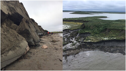
Figure 11. Shore level images of Tuktoyaktuk Island (left) and Peninsula Point (right). Note the steep slope of the Tuktoyaktuk Island coastal site, which shows undercutting caused by a storm surge leading to block failure. The cliff face has a sandy texture with areas of massive ice. By contrast, the Peninsula Point image shows the character of massive ice found in the headwall leading to retrogressive thaw flows, which are removed from the beach face through wave action. Also visible are the remnants (headwalls) of previously active retrogressive thaw slumps which have stabilized with the development of vegetation.

During the storm event on August 17, 2018 (D1–D2), there was minimal change in the cliff edge position at both study sites, however, the cliff toe position saw considerable landward movement. At Tutoyaktuk Island, the cliff toe retreat was largely uniform with a maximum retreat of roughly 5 m and over 55% in the 1–3 m range. At Peninsula Point, cliff toe movements were more variable commonly exceeding 5 m and up to 10 m of retreat with 26% experiencing between 0 and 1 m of landward movement. During the seasonal time step (D2–D3), the cliff toe rebounded with a net seaward movement at both study sites, which corresponds to the increase in cliff edge erosion observed over this time frame. The pattern of cliff toe and edge movements were again more uniform at Tuktoyaktuk Island than Peninsula Point, which saw a major retreat in the cliff edge of over 10 m and a large portion with little to no change (Figure 6). However, over the entire time frame (D1–D3), the cliff toe and edge exhibited the same general behavior at the respective sites (Figures 4 and 6). Over very short timescales, and in our case after the storm event, we have found that the cliff toe movement is most dominant where wave action interacts with the toe to remove sediment (Lim et al. 2020). Longer term datasets are necessary to assess the interaction of forcing factors on coastal erosion (Jones et al. 2018). The loss of the material at the base of the cliff will lead to destabilization of the cliff edge, which will then deposit new material at the base. As these processes equilibrate over time, the net move of the cliff toe and edge will begin to converge as exemplified at the Tuktoyaktuk Island study site (Figure 4). The equilibrium process is likely to be governed by site specific characteristics and complicated by unique features resulting from the presence of permafrost and excess ground ice. For instance, despite our study sites exhibiting similar exposure and being <7 km apart, the Peninsula Point coastal type is classified as a retrogressive thaw slump, contains different coastal geometry, and would explain some of the variability in our results. The cliff toe (slump lobe) and cliff edge (headwall) at Peninsula Point are spatially more distant than the traditional cliff toe-edge relationship found at Tuktoyaktuk Island and separated by a thaw flow. A similar mechanism of sediment transport would exist where material at the base would be removed by wave action and replaced by material from the cliff edge, or retreating headwall (Lim et al. 2020), but would operate at a different timescale. Further, exposed ice commonly found in the headwall of a retrogressive thaw slump would be heavily impacted by orientation, ground slope, ambient air temperatures, and solar radiation (Lewkowicz 1987), which explains the major cliff edge retreating events observed over our seasonal time scale.

There was a substantial amount of variability in the volumetric change measurements made at both study sites and no apparent relationship was observed with any of the planimetric movements of coastal boundaries as observed by Obu et al. (2016). Over the first time step (D1–D2) at Tuktoyaktuk Island where cliff toe erosion was dominant, there was consistent cliff volume loss. Over the second time step, cliff edge erosion dominated and corresponded with consistent cliff volume loss. Over the study timeframe (D1–D3), there was a loss of beach and cliff volume along the majority of measurement transects, which is consistent with the net cliff toe and edge erosion observed despite an overall widening of the beach. Overall, at Tuktoyaktuk Island, it was observed that small amounts of planimetric retreat can correspond to large volumetric changes in the coastal cliff and beach sediments. Annual volumetric erosion between 2000 and 2018 of the cliff face at Tuktoyaktuk Island has been calculated as 6663 m³/year (Whalen et al. 2022), which is consistent with our calculation of cliff volume erosion of 8609 m³ between 2018 and 2019. The discrepancy is likely a result of inter-annual variability and sampling resolution. At Peninsula Point, where the temporal scale of coastal processes differs, the volumetric changes, particularly the cliff volume, are considerably variable. There is a consistent retreat of the cliff toe and edge, corresponding to cliff volume loss. The majority of beach volume loss is between ±3 m³/m (Figure 6), which is consistent with a relatively stable waterline suggesting that sediment is quickly transported into the nearshore and eventually offshore. The cliff segments at Peninsula Point are long and in effect characterize the volume of the retrogressive thaw slump floor and because sediment transport can move laterally between volume segments, the total volume change per segment may be the consequence of eroded material bounded by adjacent segments. A similar study by Lim et al. (2020) calculating storm driven and annual volume change at Peninsula Point a year later, also found there to be more volume change occurring over the longer annual time step where 28% of the volume loss occurred during the storm event and 72% occurring over the remainder of the ice-free days. Despite the overall higher magnitude of volume loss found by Lim et al. (2020) a year later, the relative percentages were similar where we found 24% of the volume loss occurring during the storm event and 76% occurring during the remainder of the open water season. Lim et al. (2020) noted the majority of volume change at Peninsula Point was concentrated at the exposed massive ice and permafrost cliffs. As a result of our analysis, we restricted our calculations of change to the coastal zone to limit errors associated with UAV-SfM reconstruction which can suggest an apparent change in unchanging areas between surfaces (James et al. 2017). Further, we calculated volume change based on change envelope segments and differentiated between beach and cliff volume change adding sophistication to the volume change calculations highlighting the importance of geomorphic context in applying and interpreting rates of change (Lim et al. 2020).

GEOBIA feature extraction

When comparing coastal features extracted using GEOBIA to features extracted using manual identification, we found there to be similarities between study sites. Specifically, there was poor agreement between the waterline features, at both sites, with reasonable agreement between cliff toe and cliff edge features (Figures 8–10). The waterline is generally less well-defined, and fuzzy, compared to a cliff toe or edge and temporally variable during data collection due to wave action and tidal differences between datasets. Depending on the beach topography, a high water mark can create an image object that is spectrally similar to the mean waterline, which is difficult to differentiate using a GEOBIA rule set and can even introduce subjectivity during manual delineation. Further, UAV-SfM is known to be ineffective in reconstructing water surfaces due to the movement of tie points (Carrivick et al. 2016) and less accurate at the boundaries of a survey area due to reduced image overlap (Colomina and Molina 2014). For these reasons, it is likely that a waterline feature contains inherent errors that other features may not, which will impact the segmentation of meaningful image objects using GEOBIA and introduce inaccuracies when manually digitizing UAV-SfM imagery. Of the six total waterline feature extraction comparison scenarios, four had an average difference of >2 m (Figures 9 and 10). The D2 and D3 scenarios at Peninsula Point provided improved results in waterline extraction and can be attributed to a more defined waterline (i.e., mean waterline equals high water line).

At the Tuktoyaktuk Island study site there tended to be less variability in reported average differences in feature extraction between temporal datasets whereas at the Peninsula Point study site, the dataset influenced reported averages, particularly for the cliff toe and edge features. The study site at Peninsula Point can also be considered a more complex coastal zone than that of Tuktoyaktuk Island which contributes to anomalous regions. Besides the presence of ice found in the permafrost at Tuktoyaktuk Island, this coastal zone is considered to have a coastal cliff or bluff classification whereas the Peninsula Point coastal study site is made up entirely of an active retrogressive thaw slump. The result is a more straightforward identification of coastal features at Tuktoyaktuk Island for both manual delineation and using GEOBIA rule sets. At Peninsula Point, there are active flows that influence the interpretation of the cliff toe position and areas of exposed massive ice in the cliff face resulted in misclassification with GEOBIA feature extraction. The proposed algorithms were developed specifically for the highly erosional coastal types of our study sites and are not likely directly applicable to other Arctic coastal environments. Our algorithms relied on the slope, derived from the DSMs, characteristics of the study sites, which contained steep slopes. As a result, the availability of a DEM is necessary and may not be as applicable to a gradual sloping coastal environment. The use of indices for classifying vegetation and water, however, is likely to be widely applicable across Arctic coasts. Indices will also minimize potential offsets due to imagery collected using different sensors.

The rule sets developed were modified slightly between study sites. At Tuktoyaktuk Island, more emphasis was given to spectral characteristics by using a modified vegetation index. At Peninsula Point, more emphasis was given to geomorphometrics by utilizing elevation and slope as key indicators for feature extraction. This explains the similarity in D1 and D2 results at Tuktoyaktuk Island and the relative difference of D3. D1 and D2 are separated by only 9 days, therefore, the vegetation exhibited similar characteristics. Lighting conditions varied slightly between D1 and D2 resulting in a shadow cast onto the beach by the cliff in D2 causing some anomalous areas in cliff toe comparison. D3, however, was captured in the early summer as opposed to D1 and D2 being captured during the mid to late summer. This resulted in considerable differences in the vegetation reflectance values between datasets and had the greatest impact on the extraction of the cliff edge. During early summer, when vegetation is brown in color, there is a smaller spectral difference between the tundra vegetation and sediment of the cliff, and can create erroneous images objects resulting from poor image segmentation. The contrast between cliff sediment and beach sediment is less dependent on the time of year and did not negatively impact GEOBIA feature extraction accuracy. While not utilized here, the use of more sophisticated multispectral sensors with near-infrared or red edge bands, as opposed to RGB sensors, might provide improved feature extraction accuracies and mitigate issues caused by temporal variability. Further utilizing surface parameters, such as elevation and slope would improve extraction accuracies as exemplified by the results obtained at the Peninsula Point study site.

Conclusion

Geomorphic response to a coastal storm event and seasonal changes at two spatially similar study sites were quantified and were shown to exhibit different behavior. By tracking the temporal change of multiple coastal indicators features along a common set of transects and creating volume change envelope segments, we were able to show that the coastal change of different coastal types can occur at different time scales and that the choice in coastal indicator feature used to measure coastal erosion along Arctic coasts influences reported movements over short time scales.

At the Tuktoyaktuk Island study site, the majority of erosion of the cliff toe occurred during a storm event and remained stable, or accreted, over a seasonal time scale while the cliff edge remained stable during the storm event and retreated landward over the seasonal time scale. At the Peninsula Point study site, the cliff toe/edge relationship was less symbiotic due to the polycyclic retrogressive thaw slump dominating the site. Here, the cliff toe and edge (i.e., the headwall) were spatially distant and were influenced by different forcing factors. The cliff toe was influenced by wave action and the cliff edge was influenced by the melting of exposed ice and subsequent flow of material through the slump floor. At both study sites the waterline boundary was found to move seaward along the majority of measurement transects resulting from the deposition of sediment from eroding cliffs.

Volumetric change measurements reported on a per meter basis of the cliff were found to be highest following the storm surge event at the Tuktoyaktuk Island study site but considerably more variable at the Peninsula Point study site, over all time steps due to the complex behavior of sediment through coastal retrogressive thaw slumps. Further, we found the reported planimetric movements and volumetric change to be variable across the analyzed coastal retrogressive thaw slump environment highlighting the potential challenges presented in accurately quantifying the volumetric erosion of Arctic coasts.

When GEOBIA derived datasets were compared against manual interpretations of three coastal features, the GEOBIA datasets were found to be more accurate for measuring the position of the cliff toe (0.52, 0.6 m) and cliff edge (0.65, 0.75 m) than the waterline (3.25, 1.68 m). The temporal variability of the waterline can lead to misclassification and UAV-SfM reconstruction limitations of water features creates data artifacts and unreliable interpretations. Also, the influence of data collection date was more apparent at the Tuktoyaktuk Island study site, which utilized a vegetation index based on spectral bands than at the Peninsula Point study site, which emphasized geomorphometrics. The index-based approach meant that the difference between vegetation and sediment was less discernable in spring than in summer. As the temporal variations in spectral reflectance are very apparent, the implementation of automatic threshold calculation may be a viable solution in future work. A geomorphometric based approach is not temporally dependent and can distinguish between classes based on changes in elevation and slope. More sophisticated DSM derivatives, such as slope curvature, would be useful for the segmentation and/or classification and are worthwhile considering in future work. By using the boundary lines between classes identified using a GEOBIA approach we were successfully able to identify the cliff toe and cliff edge coastal features across temporal datasets to within an acceptable margin of error of the coastal features identified using expert manual interpretation representing a potentially viable alternative to traditional forms of coastline delineation.

GEOBIA presents a systematic approach to coastline extraction and classification that can be applied to data stacks, potentially reducing the requirements of labor intensive manual delineation by multiple interpreters, which will be of particular importance for large scale, high temporal, monitoring of Arctic coasts. Further, a GEOBIA approach can contribute to the investigation of short term, multi-feature, coastal dynamics in the Arctic as well as large scale monitoring. As one of the first applications of GEOBIA to Arctic coasts on UAV-SfM datasets, the results presented are encouraging but require further research to be fully realized. Further refinement of rule sets where 3D data is available (i.e., UAV-SfM) should focus on geomorphometrics rather than spectral indices and the use of multispectral sensors (i.e., satellite imagery) should be investigated, which could significantly improve waterline extraction and improve vegetation, non-vegetation classifications. Further, deep learning approaches have the potential for extracting coastal geomorphic boundaries and may be well-suited for future work looking to broad scale object-based Arctic coastal feature extraction. We were able to effectively characterize coastal features at the local scale but we recommend our object-based approach extend to large scale coastal scenes, lower resolution imagery, and explore the use of supervised classification and machine learning techniques for coastal classification.

Acknowledgments

We are grateful to the field crews, community members, and NRCan staff who worked on this project during the 2018 and 2019 field surveys, in particular, Angus Robertson, Paul Fraser, and Bay Berry for their contributions to the field logistics, and data collection. We would also like to acknowledge the community of Tuktoyaktuk, the Tuktoyaktuk Community Corporation, and the Tuktoyaktuk Hunters and Trappers Committee for their continued support. Permitting for this project fell under the NWT Science Licences: 16073 and 16286. Inuvialuit land administration land use permit ILA18TN005 and Parks Canada Research and Collection Permit PCL-2018-2761-02.

Disclosure statement

No potential conflict of interest was reported by the author(s).

Additional information

Funding

This research was funded by the Climate Change Geoscience Program (Natural Resources Canada), Crown-Indigenous Relations and Northern Affairs Canada (CIRNAC): (1) Climate Change preparedness in the North (CCPN); (2) Beaufort Sea Regional Strategic Environmental Assessment (BRSEA). As well, it was funded by a Natural Science and Engineering Council of Canada Discover grant and Northern supplement to BJM and by a Northern Student Training Program from Polar Knowledge Canada to AC.

References

- Berry, H.B., Whalen, D., and Lim, M. 2021. “Long-term ice-rich permafrost coast sensitivity to air temperatures and storm influence: Lessons from Pullen Island, Northwest Territories, Canada.” Arctic Science, Vol. 7(No. 4): pp. 723–745. doi:10.1139/as-2020-0003.
- Blaschke, T. 2010. “Object based image analysis for remote sensing.” ISPRS Journal of Photogrammetry and Remote Sensing, Vol. 65(No. 1): pp. 2–16. doi:10.1016/j.isprsjprs.2009.06.004.
- Carrivick, J.L., Smith, M.W., and Quincey, D.J. 2016. Structure from Motion in the Geosciences. Hoboken, GB: Wiley-Blackwell. doi:10.1002/9781118895818.
- Castilla, G., and Hay, G.J. 2008. “Image objects and geographic objects.” In Object-Based Image Analysis. Lecture Notes in Geoinformation and Cartography, edited by T. Blaschke, S. Lang, and G.J. Hay, 91–110. Berlin; Heidelberg: Springer. doi:10.1007/978-3-540-77058-9_5.
- Chen, G., Weng, Q., Hay, G.J., and He, Y. 2018. “Geographic object-based image analysis (GEOBIA): Emerging trends and future opportunities.” GIScience & Remote Sensing, Vol. 55(No. 2): pp. 159–182. doi:10.1080/15481603.2018.1426092.
- Clark, A., Moorman, B., Whalen, D., and Fraser, P. 2021. “Arctic coastal erosion: UAV-SfM data collection strategies for planimetric and volumetric measurements.” Arctic Science, Vol. 7(No. 3): pp. 605–633. doi:10.1139/as-2020-0021.
- Clark, A., Moorman, B., Whalen, D., and Vieira, G. 2022. “Multiscale object-based classification and feature extraction along Arctic coasts.” Remote Sensing, Vol. 14(No. 13): pp. 2982. doi:10.3390/rs14132982.
- Colomina, I., and Molina, P. 2014. “Unmanned aerial systems for photogrammetry and remote sensing: A review.” ISPRS Journal of Photogrammetry and Remote Sensing, Vol. 92: pp. 79–97. doi:10.1016/j.isprsjprs.2014.02.013.
- Cunliffe, A.M., Tanski, G., Radosavljevic, B., Palmer, W.F., Sachs, T., Lantuit, H., Kerby, J.T., and Myers-Smith, I.H. 2019. “Rapid retreat of permafrost coastline observed with aerial drone photogrammetry.” The Cryosphere, Vol. 13(No. 5): pp. 1513–1528. doi:10.5194/tc-13-1513-2019.
- Dallimore, S.R., Wolfe, S.A., and Solomon, S.M. 1996. “Influence of ground ice and permafrost on coastal evolution, Richards Island, Beaufort Sea coast.” Canadian Journal of Earth Sciences, Vol. 33(No. 5): pp. 664–675. doi:10.1139/e96-050.
- Environment and Climate Change Canada. 2020. Hourly data (Jul 2020) – Climate ID 2203911 – Tuktoyaktuk A, Northwest Territories [Table]. Available from https://climate.weather.gc.ca/historical_data/search_historic_data_e.html.
- Forbes, D.L., and Frobel, D. 1985. Coastal erosion and sedimentation in the Canadian Beaufort Sea. In Current research, part B. Geological Survey of Canada, paper 85-1B, pp. 69–80.
- Forbes, D.L., Manson, G.K., Whalen, D.J.R., Couture, N.J., and Hill, P.R. 2014. “Coastal products of marine transgression in cold-temperate and high-latitude coastal-plain settings: Gulf of St Lawrence and Beaufort Sea.” Geological Society, London, Special Publications, Vol. 388(No. 1): pp. 131–163. doi:10.1144/SP388.18.
- Ford, J.D., McDowell, G., and Pearce, T. 2015. “The adaptation challenge in the Arctic.” Nature Climate Change, Vol. 5(No. 12): pp. 1046–1053. doi:10.1038/nclimate2723.
- Fritz, M., Vonk, J.E., and Lantuit, H. 2017. “Collapsing Arctic coastlines.” Nature Climate Change, Vol. 7(No. 1): pp. 6–7. doi:10.1038/nclimate3188.
- Gitelson, A.A., Kaufman, Y.J., Stark, R., and Rundquist, D. 2002. “Novel algorithms for remote estimation of vegetation fraction.” Remote Sensing of Environment, Vol. 80(No. 1): pp. 76–87. doi:10.1016/S0034-4257(01)00289-9.
- Günther, F., Overduin, P.P., Sandakov, A.V., Grosse, G., and Grigoriev, M.N. 2013. “Short- and long-term thermo-erosion of ice-rich permafrost coasts in the Laptev Sea region.” Biogeosciences, Vol. 10(No. 6): pp. 4297–4318. doi:10.5194/bg-10-4297-2013.
- Günther, F., Overduin, P.P., Yakshina, I.A., Opel, T., Baranskaya, A.V., and Grigoriev, M.N. 2015. “Observing Muostakh disappear: Permafrost thaw subsidence and erosion of a ground-ice-rich island in response to arctic summer warming and sea ice reduction.” The Cryosphere, Vol. 9(No. 1): pp. 151–178. doi:10.5194/tc-9-151-2015.
- Harper, J.R. 1990. “Morphology of the Canadian Beaufort Sea coast.” Marine Geology, Vol. 91(No. 1–2): pp. 75–91. doi:10.1016/0025-3227(90)90134-6.
- Hay, G.J., and Castilla, G. 2008. Geographic object-based image analysis (GEOBIA): A new name for a new discipline. In Object-Based Image Analysis. Lecture Notes in Geoinformation and Cartography, edited by T. Blaschke, S. Lang, and G.J. Hay. Berlin; Heidelberg: Springer. doi:10.1007/978-3-540-77058-9_4.
- Hidayat, F., Rudiastuti, A.W., and Purwono, N. 2018. “GEOBIA an (geographic) object-based image analysis for coastal mapping in Indonesia: A review.” IOP Conference Series: Earth and Environmental Science, Vol. 162(No. 1): pp. 012039. doi:10.1088/1755-1315/162/1/012039.
- Hill, P.R., Blasco, S.M., Harper, J.R., and Fissel, D.B. 1991. “Sedimentation on the Canadian Beaufort Shelf.” Continental Shelf Research, Vol. 11(No. 8–10): pp. 821–842. doi:10.1016/0278-4343(91)90081-G.
- Irrgang, A.M., Lantuit, H., Manson, G.K., Günther, F., Grosse, G., and Overduin, P.P. 2018. “Variability in Rates of Coastal Change Along the Yukon Coast, 1951 to 2015.” Journal of Geophysical Research: Earth Surface, Vol. 123(No. 4): pp. 779–800. doi:10.1002/2017JF004326.
- James, M.R., Robson, S., and Smith, M.W. 2017. “3-D uncertainty-based topographic change detection with structure-from-motion photogrammetry: Precision maps for ground control and directly georeferenced surveys.” Earth Surface Processes and Landforms, Vol. 42(No. 12): pp. 1769–1788. doi:10.1002/esp.4125.
- James, M.R., Chandler, J.H., Eltner, A., Fraser, C., Miller, P.E., Mills, J.P., Noble, T., Robson, S., and Lane, S.N. 2019. “Guidelines on the use of structure-from-motion photogrammetry in geomorphic research.” Earth Surface Processes and Landforms, Vol. 44(No. 10): pp. 2081–2084. doi:10.1002/esp.4637.
- Jones, B.M., Arp, C.D., Jorgenson, M.T., Hinkel, K.M., Schmutz, J.A., and Flint, P.L. 2009. “Increase in the rate and uniformity of coastline erosion in Arctic Alaska.” Geophysical Research Letters, Vol. 36, L03503. doi:10.1029/2008GL036205.
- Jones, B.M., Farquharson, L.M., Baughman, C.A., Buzard, R.M., Arp, C.D., Grosse, G., Bull, D.L., Günther, F., Nitze, I.; Urban, F., et al. 2018. A decade of remotely sensed observations highlight complex processes linked to coastal permafrost bluff erosion in the arctic. Environmental Research Letters, Vol. 13: pp. 115001. doi:10.1088/1748-9326/aae471.
- Jorgenson, M.T., Shur, Y.L., and Pullman, E.R. 2006. “Abrupt increase in permafrost degradation in Arctic Alaska.” Geophysical Research Letters, Vol. 33. doi:10.1029/2005GL024960.
- Judge, A.S., Pelletier, B.R., and Norquay, I. 1987. “Permafrost base and distribution of gas hydrates.” In Marine Science Atlas of the Beaufort Sea-Geology and Geophysics. Geological Survey of Canada, Miscellaneous Report 40, 39.
- Kim, J., Murphy, E., Nistor, I., Ferguson, S., and Provan, M. 2021. “Numerical analysis of storm surges on Canada’s western Arctic coastline.” Journal of Marine Science and Engineering, Vol. 9(No. 3): pp. 326. doi:10.3390/jmse9030326.
- Lantuit, H., and Pollard, W.H. 2008. “Fifty years of coastal erosion and retrogressive thaw slump activity on Herschel Island, southern Beaufort Sea, Yukon Territory, Canada.” Geomorphology, Vol. 95(No. 1–2): pp. 84–102. doi:10.1016/j.geomorph.2006.07.040.
- Lantuit, H., Overduin, P.P., Couture, N., Wetterich, S., Aré, F., Atkinson, D., Brown, J., et al. 2012. “The Arctic coastal dynamics database: A new classification scheme and statistics on Arctic permafrost coastlines.” Estuaries and Coasts, Vol. 35(No. 2): pp. 383–400. doi:10.1007/s12237-010-9362-6.
- Lewkowicz, A.G. 1987. “Headwall retreat of ground-ice slumps, Banks Island, Northwest Territories.” Canadian Journal of Earth Sciences, Vol. 24(No. 6): pp. 1077–1085. doi:10.1139/e87-105.
- Lim, M., Whalen, D., J. Mann, P., Fraser, P., Berry, H.B., Irish, C., Cockney, K., and Woodward, J. 2020. “Effective monitoring of permafrost coast erosion: Wide-scale storm impacts on outer islands in the Mackenzie Delta Area.” Frontiers in Earth Science, Vol. 8: pp. 1–17. doi:10.3389/feart.2020.561322.
- Lindsay, R., and Schweiger, A. 2015. “Arctic sea ice thickness loss determined using subsurface, aircraft, and satellite observations.” The Cryosphere, Vol. 9(No. 1): pp. 269–283. doi:10.5194/tc-9-269-2015.
- Mackay, J.R. 1986. Fifty years (1935-1985) of coastal retreat west of Tuktoyaktuk, District of Mackenzie. Geological Survey of Canada, Paper 86-1A, pp. 727–735.
- Mackay, J.R., and Burn, C.R. 2002. “The first 20 years (1978–1979 to 1998–1999) of ice-wedge growth at the Illisarvik experimental drained lake site, western Arctic coast, Canada.” Canadian Journal of Earth Sciences, Vol. 39(No. 1): pp. 95–111. doi:10.1139/e01-048.
- Malenfant, F., Whalen, D., Fraser, P., and van Proosdij, D. 2022. “Rapid coastal erosion of ice-bonded deposits on Pelly Island, southeastern Beaufort Sea, Inuvialuit Settlement Region, western Canadian Arctic.” Canadian Journal of Earth Sciences, Vol. 59(No. 11): pp. 961–972. doi:10.1139/cjes-2021-0118.
- Manson, G.K., Solomon, A.S.M., Forbes, A.D.L., Atkinson, D.E., and Craymer, A.M. 2005. “Spatial variability of factors influencing coastal change in the Western Canadian Arctic.” Geo-Marine Letters, Vol. 25(No. 2–3): pp. 138–145. doi:10.1007/s00367-004-0195-9.
- Mars, J.C., and Houseknecht, D.W. 2007. “Quantitative remote sensing study indicates doubling of coastal erosion rate in past 50 yr along a segment of the Arctic coast of Alaska.” Geology, Vol. 35(No. 7): pp. 583–586. doi:10.1130/G23672A.1.
- Meier, W.N., Hovelsrud, G.K., van Oort, B.E.H., Key, J.R., Kovacs, K.M., Michel, C., Haas, C., et al. 2014. “Arctic sea ice in transformation: A review of recent observed changes and impacts on biology and human activity.” Reviews of Geophysics, Vol. 52(No. 3): pp. 185–217. doi:10.1002/2013RG000431.
- Moorman, B. 1998. The Development and Preservation of Tabular Massive Ground Ice in Permafrost Regions. PhD Dissertation. Ottawa: Carleton University, 308.
- Nielsen, D.M., Pieper, P., Barkhordarian, A., Overduin, P., Ilyina, T., Brovkin, V., Baehr, J., and Dobrynin, M. 2022. “Increase in Arctic coastal erosion and its sensitivity to warming in the twenty-first century.” Nature Climate Change, Vol. 12(No. 3): pp. 263–270. doi:10.1038/s41558-022-01281-0.
- Obu, J., Lantuit, H., Fritz, M., Pollard, W.H., Sachs, T., and Günther, F. 2016. “Relation between planimetric and volumetric measurements of permafrost coast erosion: A case study from Herschel Island, western Canadian Arctic.” Polar Research, Vol. 35(No. 1): pp. 30313. doi:10.3402/polar.v35.30313.
- Overeem, I., Anderson, R.S., Wobus, C.W., Clow, G.D., Urban, F.E., and Matell, N. 2011. “Sea ice loss enhances wave action at the Arctic coast.” Geophysical Research Letters, Vol. 38(No. 17). doi:10.1029/2011GL048681.
- Papakonstantinou, A., Topouzelis, K., and Pavlogeorgatos, G. 2016. “Coastline zones identification and 3D coastal mapping using UAV spatial data.” ISPRS International Journal of Geo-Information, Vol. 5(No. 6): pp. 75. doi:10.3390/ijgi5060075.
- Radosavljevic, B., Lantuit, H., Pollard, W., Overduin, P., Couture, N., Sachs, T., Helm, V., and Fritz, M. 2016. “Erosion and flooding threats to coastal infrastructure in the Arctic: A case study from Herschel Island, Yukon Territory, Canada.” Estuaries and Coasts, Vol. 39(No. 4): pp. 900–915. doi:10.1007/s12237-015-0046-0.
- Ramage, J.L., Irrgang, A.M., Herzschuh, U., Morgenstern, A., Couture, N., and Lantuit, H. 2017. “Terrain controls on the occurrence of coastal retrogressive thaw slumps along the Yukon Coast, Canada.” Journal of Geophysical Research: Earth Surface, Vol. 122(No. 9): pp. 1619–1634. doi:10.1002/2017JF004231.
- Río, L.D., and Gracia, F.J. 2013. “Error determination in the photogrammetric assessment of shoreline changes.” Natural Hazards, Vol. 65(No. 3): pp. 2385–2397. doi:10.1007/s11069-012-0407-y.
- Semiletov, I., Pipko, I., Gustafsson, Ö., Anderson, L.G., Sergienko, V., Pugach, S., Dudarev, O., et al. 2016. “Acidification of East Siberian Arctic Shelf waters through addition of freshwater and terrestrial carbon.” Nature Geoscience, Vol. 9(No. 5): pp. 361–365. doi:10.1038/ngeo2695.
- Solomon, S.M. 2005. “Spatial and temporal variability of shoreline change in the Beaufort-Mackenzie region, northwest territories, Canada.” Geo-Marine Letters, Vol. 25(No. 2–3): pp. 127–137. doi:10.1007/s00367-004-0194-x.
- Solomon, S.M., Forbes, D.L., and Kierstead, B. 1994. Coastal impacts of climate change: Beaufort Sea erosion study. Atmospheric Environment Service, Canadian Climate Centre, Report 94-2. Geological Survey of Canada, Open File 2890, 85 pp.
- Stocker, T., Qin, D., Plattner, G.-K., Tignor, M., Allen, S.K., Boschung, J., Nauels, A., Xia, Y., Bex, V., and Midgley, P.M. 2013. “Climate change 2013: The physical science basis.” In Contribution of Working Group I to the Fifth Assessment Report of the Intergovernmental Panel on Climate Change. Cambridge: Cambridge University Press.
- Tanski, G., Wagner, D., Knoblauch, C., Fritz, M., Sachs, T., and Lantuit, H. 2019. “Rapid CO2 release from eroding permafrost in seawater.” Geophysical Research Letters, Vol. 46(No. 20): pp. 11244–11252. doi:10.1029/2019GL084303.
- Thieler, E.R., Himmelstoss, E.A., Zichichi, J.L., and Ergul, A. 2009. The Digital Shoreline Analysis System (DSAS) Version 4.0 – An ArcGIS extension for calculating shoreline change (Version 5.0, October 2019). USGS Numbered Series, U.S. Geological Survey, Reston, Open-File Report 2008-1278. doi:10.3133/ofr20081278.
- Whalen, D., Forbes, D.L., Kostylev, V., Lim, M., Fraser, P., Nedimović, M.R., and Stuckey, S. 2022. “Mechanisms, volumetric assessment, and prognosis for rapid coastal erosion of Tuktoyaktuk Island, an important natural barrier for the harbour and community.” Canadian Journal of Earth Sciences, Vol. 59(No. 11): pp. 945–960. doi:10.1139/cjes-2021-0101.