An Exploration of False Positives Following Multispectral Analysis of Mine Tailings Extent

Abstract

Satellite imagery can be analyzed to offer a preliminary regional assessment of mine tailings indicators, enabling identification before performing in-depth fieldwork. Nova Scotia, Canada, still retains mine tailings produced in the 1860s to the 1940s in 64 historic gold districts, which exceed soil guidelines for arsenic (As) and mercury (Hg) levels. Tailings data often relies on historical maps, which may not accurately depict the current extent due to wind and rain transportation. A classification model was designed to analyze multispectral Sentinel-2 images and indicate pixels potentially comprising tailings. This classifier had an overall F1-Score about 0.7 for most methods tested, but this accuracy was not consistent across all land cover types. In particular, wetland and coastal areas seemed to generate a high number of false positives. In this study, these potential false positives are investigated to better understand the model’s confusion and improve future results.

résume

L’imagerie satellitaire peut offrir une évaluation régionale préliminaire des indicateurs de résidus miniers, ce qui permet une identification avant d’effectuer un travail de terrain approfondi. Au Canada, la Nouvelle-Écosse a encore de nombreux résidus miniers qui ont été produits entre les années 1860 et 1940 dans 64 districts aurifères historiques. Les sols de ces résidus ont des teneurs en arsenic (As) et mercure (Hg) qui dépassent les normes recommandées Les données sur les résidus proviennent souvent de cartes historiques, qui peuvent ne pas représenter avec précision l’étendue actuelle des résidus à cause du transport par le vent et les précipitations. On a développé un modèle de classification pour analyser les images multispectrales Sentinel-2 afin de cartographier les pixels correspondant potentiellement aux résidus. Ce classificateur avait un score F1 global d’environ 0,7 pour la plupart des méthodes testées, mais cette précision n’était pas uniforme pour tous les types de couverture au sol. En particulier, les zones humides et côtières semblaient générer un nombre élevé de faux positifs. Dans cette étude, ces faux positifs potentiels sont étudiés afin de mieux comprendre la confusion du modèle et d’améliorer les résultats futurs.

Introduction

Mines operating in the nineteenth to mid-twentieth centuries throughout Nova Scotia, Canada have left behind tailings containing arsenic (As) and mercury (Hg). These sites have been identified as an ongoing source of contamination and a threat to human and ecosystem health since the 1970s when the first cases of As intoxication from mine-impacted drinking water were reported (Hindmarsh et al. 1977). Ongoing surveys at additional historic mine sites have revealed that at some sites, tailings have moved downstream from their original locations to be deposited in lakes, riverbanks, and estuaries (Koch et al. 2007; Parsons et al. 2012). Over 300 gold mines have operated in the province, organized into 64 gold mine districts. Before sites can be cleaned up, they must first be assessed to determine whether tailings are present, and where.

Remote sensing methods can provide a preliminary assessment of historic mine sites, quickly analyzing large areas to indicate where tailings may be present. We trained a random forest classifier using historical maps of tailings and multispectral Sentinel-2 images so that indicators of tailings could be mapped across multiple gold mine districts. Pixel-wise classification accuracy was tested by repeating classification and recording the distribution of results (Jewell 2024). By separating the results by district, we determined that accuracy among them was inconsistent. The classifier performed poorly at sites with significant areas of standing water and shorelines, even after filtering satellite images to the driest season (July and August). In this study, we compare the spectra, as provided by Sentinel-2, of areas where the classifier provided false positives, as confirmed by lab analysis of sediment. We also present scanning electron microscope (SEM) analysis and bulk geochemistry of sediment collected from coastal and wetland areas, which are commonly confused by the classifier with tailings, and compare these sediments to tailings.

Historic gold mining and modern secondary minerals

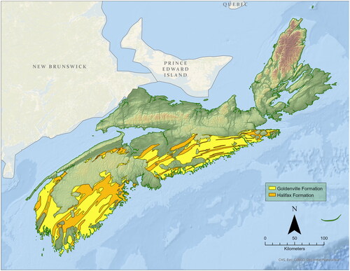
Most of the gold in Nova Scotia has historically been mined in the Goldenville and Halifax formations of the Meguma Supergroup, which is exposed throughout the southern mainland of the province (Figure 1). The high-grade gold deposits that were the main target of historic mining are found in quartz veins in the hinges of east-west trending folds, where gold has been concentrated by hydrothermal activity (Parsons et al. 2012; Sangster, Smith, and Goodfellow 2007). Sulfide minerals also present in these hinges have been the main source of arsenic (As) and acid rock drainage released by mining and processing, and present a threat to human and ecosystem health (Ngole-Jeme and Fantke 2017; Walker et al. 2009). The most common sulfide mineral found at these mine sites is arsenopyrite (FeAsS), which has been observed to comprise up to 15% of gold-bearing quartz veins (Sangster, Smith, and Goodfellow 2007). Generally, lode gold deposits like those found in Nova Scotia can be expected to contain up to three to five percent sulfide minerals (DeSisto, Jamieson, and Parsons 2016; Groves et al. 1998).

Figure 1. A map showing the province of Nova Scotia, with the Goldenville and Halifax formations overlaid. These are the main gold-bearing formations in the province.

Ore was mainly extracted from underground shafts and was then crushed in stamp mills. In many cases, particularly in the nineteenth century, mercury (Hg) was used to separate gold from crushed material in a process called mercury amalgamation (Bates 1987; LeBlanc et al. 2020; Parsons et al. 2012). The leftover waste rock and sand to silt-sized sediment, called tailings, was deposited in streams, wetlands, or nearby depressions with little to no regard for potential environmental impacts (Drage 2015; LeBlanc et al. 2020). In these tailings areas, sulfide minerals have been exposed to oxygen and surface water, leading to oxidation and dissolution of As and metals (DeSisto, Jamieson, and Parsons 2017). Fine particles in tailings are susceptible to eolian and fluvial transportation, spreading As and Hg beyond tailings areas (Cleaver et al. 2021). For example, at Lower Seal Harbor a large tailings deposit was discovered over two kilometers downstream of the original tailings area (Parsons et al. 2012). An estimated three million tonnes of tailings were produced across all districts (Parsons et al. 2012), most of which have sat untouched since their deposition, except for off road vehicle use at some sites.

Historical gold mine tailings mineralogy

Though no two sites have identical mineralogy, the historic gold mine sites of mainland Nova Scotia share similar bedrock geology and processing methods. Most mines targeted auriferous quartz veins present in quartzite, slate, and metasiltstone. Present in smaller amounts are chlorite, biotite, muscovite, and plagioclase, alongside carbonates and sulfides (Walker et al. 2009). Long-term storage of tailings was not regulated in this period, and tailings were routinely left unmanaged and exposed to the environment. Up to a century of oxidation, reduction, dissolution, and precipitation have been at work at these locations, altering original mineralogy and producing a suite of secondary minerals.

Tailings mineralogy fluctuates spatially, as well as at depth. Minerals and controls on precipitation are guided mainly by whether an environment is oxidizing or reducing, which is closely related to pH. Acidity varies widely within individual tailings sites, based on surface type (e.g., tailings, mining concentrates, hardpan). A study of pore and surface water at Montague showed a pH between 2.43 and 7.13 (DeSisto, Jamieson, and Parsons 2011).

In oxidizing conditions, arsenopyrite will dissolve, releasing As into pore water and lowering pH. Pore water As may be incorporated into Fe arsenates (commonly scorodite), arsenate sulfates, Fe oxyhydroxides, Mn oxides, and Ca(Fe) arsenates (DeSisto, Jamieson, and Parsons 2016). It may also be adsorbed onto Fe oxyhydroxides and gangue minerals. The conditions for this dissolution and precipitation may only be present in microenvironments found throughout the tailings areas (DeSisto, Jamieson, and Parsons 2011).

In reducing conditions typical of subsurface tailings, sulfides will be more stable. Arsenopyrite is less likely to be dissolved, and secondary sulfides may precipitate. In these conditions, Fe and Mn oxides will be unstable and may dissolve, releasing As (DeSisto, Jamieson, and Parsons 2016).

Secondary minerals of particular interest are Fe oxides and hydroxides, which have formed in many cases as rims on sulfide minerals such as arsenopyrite. These rims were ubiquitous on arsenopyrite grains from the Montague, Oldham, and Muddy Pond tailings, as observed by SEM. For ground-truthing, we will consider sandy sediment with elevated As and weathered sulfides with Fe oxide rims to have originated from mine sites. As we will explore in the following section, these Fe oxides, in addition to being diagnostic of mine waste, also produce a spectral absorption feature that can potentially be observed in remote sensing images.

Methods

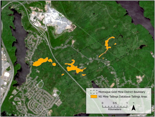
Optical remote sensing images represent the surface of the earth as pixels, combining the reflectance of all materials within that pixel to produce values at various bands. Bands represent a discrete range of the electromagnetic spectrum. Sentinel-2 surface-reflectance images were obtained in Google Earth Engine for this study. Sentinel-2 is a satellite mission operated by the European Space Agency. It comprises two nearly identical satellites, launched in 2015 and 2017 (Sentinel-2A and Sentinel-2B, respectively). The mission has a revisit period of five days or less (depending on latitude), which is the frequency at which it captures an image at a given location on Earth. These images have been georeferenced and corrected for the scattering of photons as they pass through the atmosphere (i.e., converted from “top-of-atmosphere” data as seen from space to represent the “bottom-of-atmosphere” surface reflectance). Though some optical satellites have spatial resolutions approaching or below one meter, this still pales in comparison to handheld or lab spectrometers that can provide reflectance spectra for a very precise point on the ground or on a mineral hand sample. Sentinel-2 pixels vary in resolution based on band, and pixels in images used in this study cover 20 by 20 m on the ground (Figure 2). These are small pixels in comparison to those in images captured by past multispectral missions (e.g., the Landsat mission at 30 m), but at this resolution, a pixel will still likely capture many different surface materials. Though we would like to target Fe oxides specifically, limits in spectral and spatial resolution do not allow a high degree of precision. Instead, tailings are treated as an aggregate material.

Figure 2. A sample of a natural color Sentinel-2 image at 20 m resolution. The image shows the Montague Historic Gold Mine District as well as tailings areas polygons from the Nova Scotia Mine Tailings Database.

When a pixel contains a spectrum representing a mixture of materials, it becomes harder to pinpoint the cause, or causes, of false positive classifications. We could not collect spectra of pure tailings from within a mixed pixel, and the reflectance of a material spatially correlated to tailings may have been inadvertently captured, influencing our training class. For example, tailings consist largely of crushed quartz, and its inclusion in training pixels was inevitable, though it occurs in abundance elsewhere. Vegetation, whether at the edge of tailings or growing sparsely within it, would also be included in tailings training data. Comparing the spectra of tailings to areas that contain physically similar or co-occurring materials may indicate whether these materials are causing false positive results.

Surface materials not spatially correlated to tailings may also be falsely classified as tailings based on their spectral similarity at the resolution of the Sentinel-2 sensors. As a multispectral sensor, spectral resolution is low. Each band covers a wide range, and the apparent reflectance is resampled, or convolved, from the continuous electromagnetic spectrum to the coarse resolution of the sensor. Materials may appear to have the same reflectance signature according to Sentinel-2 when a higher resolution sensor may have detected subtle differences. This may lead to false positives.

Spectrally active minerals

Predicting the presence of a mineral or land cover type by using the reflectance spectrum of a remote sensing image pixel requires that the spectral signature of a target material be distinguishable from the background or other targets. The target, or a component of the target if it is made up of mixed spectra, must also be spectrally active. A spectrally active material contains one or more absorption features in the spectral range of interest (i.e., 400–2300 nm in this study). Absorption features are regions of the reflectance spectrum where incoming photons are absorbed, rather than reflected, producing local reflectance minima (Guha 2020). When observing spectra of mixed materials, such as land cover classes (e.g., forest, urban, tailings), absorption features of constituent materials within the class may still be present. Therefore, if a material is consistently included in a land cover type, even if that land cover type consists of many materials, the absorption may still be detected. This is called a diagnostic absorption feature. A relevant example is the iron absorption feature, where photons in Fe-bearing minerals are absorbed between ∼700 and 1000 nm (Van der Werff and Van der Meer 2015)

Identification of absorption features is limited by the spectral resolution of the sensor used. In hyperspectral image analysis, the spectral resolution is sufficient in some cases that absorption features can be used to indicate mineralogy or chemical composition (Clark et al. 2003; van der Meer 2004). Multispectral data, as obtained from Sentinel-2, lack the resolution to identify the center of an absorption feature. Sentinel-2 has 13 bands with bandwidths ranging from 15 to 185 nm. It differs in this way from hyperspectral sensors, which have contiguous bands typically with bandwidths of around 10–15 nm or less. The 13 bands were chosen carefully to fulfill specific objectives and fine-tune placement based on experience gained from similar multispectral missions such as Landsat (van der Meer, van der Werff, and van Ruitenbeek 2014). In general, Sentinel-2’s bands are narrower than Landsat’s to avoid spectral absorption due to water vapor in the atmosphere. Sentinel-2’s band 8 A (a near-infrared band centered at 865 nm) was carefully placed to avoid water vapor, target peak NIR reflectance in vegetation, and be sensitive to Fe oxides in soil (European Space Agency 2015; van der Meer, van der Werff, and van Ruitenbeek 2014; Van der Werff and Van der Meer 2015). More accurate discernment of vegetation improved the ability of this model to filter out vegetation on the surface, and Fe oxides were an important indicator when classifying tailings.

If the wavelength of an absorbed photon is within the bandwidth of a band, the reflectance value for the entire band will be lowered for that pixel. In other words, absorption cannot be detected beyond the bandwidth of a band and the overall shape of the absorption cannot be observed with this sensor. Bands 8 and 8 A (with bandwidths of 106 and 21 nm, respectively) were used to detect subtle absorptions that may indicate the iron absorption feature of Fe oxides and hydroxides. The question then was whether multispectral data from Sentinel-2 would be able to differentiate tailings from naturally occurring sand that originated from the same, or at least similar, Meguma bedrock.

The mine tailings classification model

To train the classifier, polygons of known tailings areas were overlaid on Sentinel-2 images and pixels from within those polygons were sampled. These polygons (Figure 2) were derived mainly from the Nova Scotia Mine Tailings Database (Hennick and Poole 2020), which combines historical and modern tailings data into a spatial database. This database contains a compilation of data from historical mine surveys as well as modern studies. These polygons were also used to verify the results, though the same mine districts were not used for training and validation at the same time. Before these polygons could be used to obtain training points, some filters had to be applied. The tailings database includes areas that are under vegetation and where tailings have been deposited into water bodies. Vegetated pixels were removed by producing a normalized difference vegetation index (NDVI) image and filtering out tailings pixels where the NDVI value exceeded 0.6. Similarly, pixels were removed that had a modified normalized difference water index (MNDWI) value exceeding 0.0. Threshold values were determined by observing the distribution of values and testing around the mode in steps of 0.2 A more thorough description of this process can be found in Jewell (2024). After combining the vegetation and water filters with the tailings areas in the Nova Scotia Mine Tailings Database, polygons displaying dry and bare tailings were available to sample to train the classifier.

Once the bare, dry tailings areas were established, random sample points were generated to create the tailings training class. The mine districts used to train the classifier were excluded from the areas used to validate the results, and vice versa. Data was extracted from these sample points, in the form of bands and indices, from the Sentinel-2 image pixels that they intersect.

The bands used as input were the values that were considered by the random forest classifier when labeling each pixel as tailings or non-tailings. We initially selected eight bands to use in our model. The three 60 m atmospheric bands were removed. Band 8 was also removed, as it entirely overlaps the narrower band 8 A and was therefore highly correlated. Four indexes were generated and also included: normalized difference vegetation index (NDVI), modified normalized difference water index (MNDWI), ferric iron index, and iron feature depth. An optimization then determined which variables provided the most discrimination power between tailings and non-tailings pixels. Input variables were ranked by variable importance (a metric produced by the trained random forest classifier) and removed one by one. After each test, a random subset of the training data was used to test the out-of-bag error. If out-of-bag error increased when the variable was removed, it was returned to the set. If error decreased or stayed the same without that variable, it was excluded from the final variable set. Variable importance was not recalculated each time a variable was removed. This method is called non-iterative feature elimination (Díaz-Uriarte and Alvarez de Andrés,2006 Gregorutti, Michel, and Saint-Pierre 2017). The final model used seven variables: band 3 (red), band 6 (vegetation red edge), band 7 (vegetation red edge), band 8 A (narrow near-infrared), band 12 (shortwave infrared), NDVI, and MNDWI.

Finally, a tailings spectral class was created—an averaged spectrum that the classifier used to compare against all pixels when applying labels. To create the tailings spectrum, we sampled a Sentinel-2 image in areas previously mapped as tailings in the Nova Scotia Mine Tailings Database. The tailings areas included in this database were based on maps from within the last few years, as well as historic data. As such, measures were taken to ensure that the pixels sampled had not become overgrown with vegetation, or that the mapped area was not depicting where tailings had been deposited into water bodies. Optical reflectance data only represents the top mm or less (depending on the material) of the surface (Clark and Roush 1984), so the inclusion of any pixels where the surface is covered would have introduced noise to the tailings class spectrum. An NDVI layer was generated to create a vegetation mask, where pixels with values over 0.6 were excluded from tailings sampling. Similarly, MNDWI was generated to filter out pixels which appeared to contain water. A value of 0.0 was used for the water mask, though this mask did not appear to be as effective as the vegetation mask (Jewell 2024).

An advantage of using tailings area polygons to direct sample locations, as opposed to using a static tailings spectrum, was that the training data came from within the same image that was being classified. This means regional effects that may have changed the target spectra should be accounted for in the training data. For example, morning dew or recent precipitation may lower overall absorption at the tailings surface, but these will not be isolated to just the training site. Spectral libraries can be better for identifying particular minerals, but they don’t account for the impurity of pixels that are multiple meters across. The spectra on which the classifier was trained represented modern mineralogy and incorporated mineralogical changes that have taken place since tailings were first deposited. The downside of this approach was that we could not explicitly control what spectral information was used to train the classifier, except by selecting training areas. The original hypothesis was that tailings mineralogy would be sufficiently different from other sandy sediments that it could be distinguished spectrally, even using only multispectral images. This appears to have been valid when analyzing dry sediment. False positives may have emerged when areas were included in the training dataset that should not have been, or because something (e.g., water in sediment pore space) shifted the reflectance of the false positive pixels to resemble dry tailings.

Google Earth Engine

Desktop analyses, including data pre-processing, image acquisition, image sampling, classification, and accuracy assessment, were performed in Google Earth Engine (GEE), a cloud platform created by Google for remote sensing (Gorelick et al. 2017). GEE is available via web browsers or as a Python package. GEE allows the uploading of spatial data and imagery, though there are many datasets available in its built-in library. Sentinel-2 surface reflectance images are available within GEE within a few hours of the original top-of-atmosphere images, allowing for the easy selection of images with no need for further processing. In addition to image collections, GEE has a large selection of functions that can be implemented in its JavaScript and Python APIs. Computation performed in GEE is run on Google’s cloud servers, allowing for the rapid processing of massive datasets.

Applying remote sensing model to historic gold mine sites

Three historic mine districts, Montague, Oldham, and Waverley were physically sampled to obtain mineralogy and geochemistry of known tailings. These samples were used as reference material when analyzing sediment from non-tailings areas. Tailings areas at these sites are included in the Nova Scotia Mine Tailings Database, and their mean reflectance spectra were also recorded. Sulfide grains were located within samples via SEM to determine if Fe oxide rims were present. We compared the geochemistry, SEM images, and mean spectra at each site to those of coastal areas that produced false positive results in the classifier.

Montague gold mine district

Montague Gold Mine District is located north of the city of Halifax, in central Nova Scotia (latitude: 44.714°, longitude: −63.521°). The first stamp mill was constructed there in 1865, and extraction continued in some capacity until 1940 (Parsons et al. 2012). Tailings were slurried into nearby Mitchell Brook and surrounding wetlands. Tailings have been identified 2.5 km downstream in Lake Charles, which continues into the Shubenacadie Watershed (Clark et al. 2021; Mudroch and Clair 1986). Over 120,000 tonnes of ore were crushed during mining and processing at this site, and over 68,000 troy ounces of gold were produced. In hardpan areas, As was found to reach as high as 4.3 wt. % (DeSisto, Jamieson, and Parsons 2011; Parsons et al. 2012). Montague has been of special interest to researchers and the provincial government because of its elevated As and Hg and its direct proximity to urban and residential areas, which continue to expand closer to historic tailings (Intrinsik Corp et al., 2019, 2020).

Six samples were collected at Montague in October 2020. Bulk geochemistry indicated a mean As level of 9868 ppm. The highest concentration observed was 16,300 ppm As. SEM analysis indicated that arsenopyrite grains were common, and all of those observed showed signs of weathering, with Fe oxide minerals growing along edges and in cracks.

Oldham gold mine district

The Oldham gold mine district is 30 km northeast of Halifax (latitude: 44.921, longitude: −63.493). Mining took place from 1862 to 1910, and again from 1936 to 1942 (Lane et al. 1989). Approximately 107,000 tonnes of ore were crushed, and over 85,000 troy ounces of gold were produced (Parsons et al. 2012). Oldham, like Montague, is in the Shubenacadie Watershed, though only a small tributary, Black Brook, flows through the site (Lane et al. 1989). Tailings can be seen on the banks of the brook as it leaves the site. We did not identify any studies indicating that tailings from Oldham have reached the Shubenacadie River, which is approximately 3 km downstream.

Six tailings samples were collected in September 2020, which had a mean As concentration of 999 ppm and a maximum of 2362 ppm. Though the lowest As of the three sites, all samples exceeded the Canadian Council of Ministers of the Environment’s soil guideline of 12 ppm As (CCME 1997). Rims of Fe oxides were visible around weathered sulfide grains in SEM images.

Waverley gold mine district: Muddy Pond

There are multiple tailings areas in the Waverley district, however, this study focuses on the largest, called Muddy Pond. The district is located approximately 12 km north of Halifax (latitude: 44.787, longitude: −63.609). Over 150,000 tonnes of ore were crushed, producing 73,100 troy ounces of gold (Parsons et al. 2012). Unlike Montague and Oldham, which were relatively remote and required infrastructure to be built to accommodate workers, Waverley was already a small village when gold was first mined in the 1860s (Hartlen 1988). As such, mining was more or less continuous until the 1960s. Like the two districts previously mentioned, Waverley is in the Shubenacadie Watershed, with Muddy Pond separated from the main river by only a small wetland and tributary. This site is surrounded by residential communities, and development continues to expand.

Tailings samples from Waverley had a mean As concentration of 1921 ppm and a maximum of 2971 ppm.

Mapping indicators of tailings

Jewell 2024 describes how the areas around the Goldenville and Montague gold districts were analyzed using a model built in GEE. Every pixel of the input image in the target mine area was analyzed by the random forest classifier and assigned a label of tailings or non-tailings. The image used was captured on August 9th, 2019 at 12:20 PM, local time (this image can be viewed in Earth Engine by its ID: L2A_T20TMQ_A021472_20190802T151908).

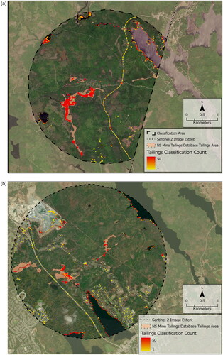
The classification model was run 50 times for each district, and results (Figure 3) were recorded using F1-score (Jewell 2024; Van Rijsbergen 1979). The 50 iterations each used a different random subset of training points and the random forest classifier generated new random values. This analysis shows the impact of randomness in the model, and shows that any single result should not be relied upon. Variance in results should always be considered when interpreting model accuracy. Maps were also generated to illustrate the frequency at which each pixel was classified as tailings (Figure 4a and 4b). These maps displayed the land cover types that most frequently elicited false positive classifications. Roads were sometimes classified as tailings, however the main sources of error were shorelines and wetlands. False positives coinciding with roads are not discussed here, as road pixels were not misclassified as consistently as the other two classes. Roads are also easier to reject as positive by an analyst, based on context and visual assessment. Being able to spectrally distinguish wetlands or shorelines that contain tailings, versus those that do not, is a more difficult task for an analyst using visual clues, and would be a valuable application of the classification model.

Figure 3. Box and whisker plot displaying F1-score at two districts. Values are spread out along the x-axis for clarity. The pixel-wise classification model was run 50 times each on Sentinel-2 images for the Goldenville and Montague regions, respectively.

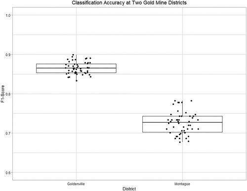
Figure 4. (a) Pixel-wise classifier at Goldenville displayed as a frequency. The model was run 50 times using a Sentinel-2 image, and the total count of positive classifications (i.e., the pixel was labeled as tailings by the classifier) is displayed in a range from 1 to 50. Where the basemap (satellite image) is shown, that pixel was never classified as tailings, and the count is 0. Image credit: Maxar. (b) Pixel-wise classifier at Montague displayed as a frequency. The model was run 50 times using a Sentinel-2 image, and the total count of positive classifications (i.e., the pixel was labeled as tailings by the classifier) is displayed in a range from 1 to 50. Where the basemap (satellite image) is shown, that pixel was never classified as tailings, and the count is 0. Image credit: Maxar.

Possible causes of positive classification

There are three likely scenarios in which wetlands and shoreline pixels would be classified as tailings, even when the area of analysis is not near a mine district:

• Polygons that were used to outline the extent of tailings and generate sample points (i.e., the training data) included wetlands and shoreline areas when they should not have. Masks were generated to remove pixels from training areas that contained water and vegetation, however, these masks (the water mask in particular) were imperfect. Therefore, when training the classifier, pixels consisting at least partially of wetlands and waterbodies may have been included. In this scenario, the classifier has inadvertently been trained to detect wetlands and shorelines, in addition to, or combination with, tailings.

• Wetlands and shoreline pixels are more likely to contain mixed spectra, and the spectral signature of these mixtures resembles that of tailings. The Sentinel-2 pixels used by the classifier are 20 by 20 m. Wetlands are a mixture of shallow water and vegetation, and these signals may combine to resemble the signal of tailings. Shorelines are typically narrow features and pixels that include them will have a reflectance signal consisting of some exposed sediment and some water (and likely vegetation). This combined signal may resemble tailings when apparent reflectance is resampled to the spectral resolution of Sentinel-2.

• The classifier was correct. Tailings were often deposited into wetlands and streams, and we should expect that tailings are still present in those areas, within and around mine sites or even up to several km downstream (Drage 2015; Parsons et al. 2012). The minimum amount of tailings required in a pixel for the classifier to correctly identify it as tailings is unknown, and hard to quantify due to many complicating factors (grain size, sediment mixture type, etc.) (Clark et al. 2003; Goetz, Curtiss, and Shiley 2009). The ability to detect tailings deposits downstream of sites along riverbanks, coastal wetlands or estuaries would be valuable, but results in these land cover types are inconsistent. Isolating the factors causing confusion in these areas would increase confidence in the results, whether positive or negative.

To explore some of these possibilities, materials identified by the classifier as tailings were sampled, both physically and spectrally, at five coastal and wetland sites. Sediment was collected at three estuarine areas downstream of multiple mine sites, as well as one wetland just north of Montague.

Sediments of estuarine environments downstream of mine districts

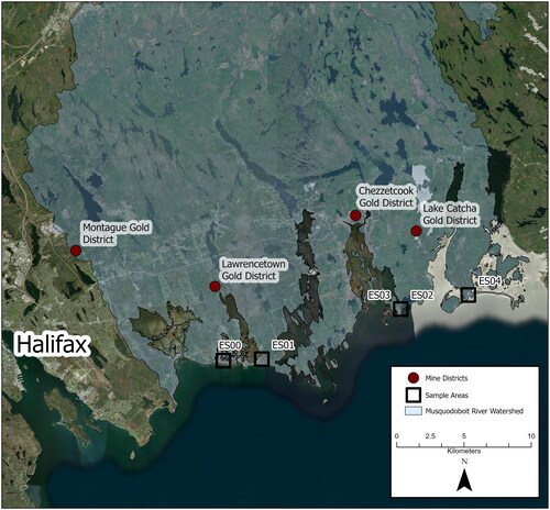
The estuarine sediment deposits were larger than the shorelines of lakes and riverbanks found near mine sites and provided purer pixels in the Sentinel-2 image, allowing us to control for pixel mixing. Lawrencetown, Lower East Chezzetcook, and Martinique Beaches were selected for sampling (Figure 5). These areas are east of Halifax, ranging from about 15 to 35 km away, along the coast. Each site consists of a narrow beach separating the ocean from salt marshes or lagoons. Samples were collected from low-energy areas, where fine sediment from upstream would be likely to be deposited. Lawrencetown and Lower East Chezzetcook are downstream of the Lawerencetown and Chezzetcook historic mine districts, respectively. These were minor districts, with Lawrencetown crushing 1534 tonnes of ore, and Chezzetcook just 73 (Parsons et al. 2012). Martinique is near the Lake Catcha historic mine district, at which 29,426 tonnes of ore was crushed. It does not appear that there are streams directly connecting this site to that mine district, making sediment transportation and deposition from there unlikely.

Figure 5. A map showing five sample sites in estuaries downstream of historic mine districts. All samples were collected in low energy areas, and are in the same watershed.

These sediment deposits, originating from the same bedrock as the gold mine districts, were presumed to be a close natural mineralogical proxy for tailings in grain size and composition. The classifier’s ability to discriminate naturally occurring sand from tailings should rely primarily on the Fe absorption feature present in Fe oxides and hydroxides. If these minerals are not present, and pure pixels are still classified as tailings, that would indicate that the classifier is including minerals that resemble tailings but do not originate from mines and may not contain high levels of As or other related contaminants. If only pixels at the beach-ocean threshold are positively classified as tailings and not the purer pixels, this would imply that false positives at shorelines are a result of pixel mixing. First, we explore if the estuarine sediment deposits contain those Fe oxides and hydroxides.

Grains from the three coastal sites were analyzed via SEM. A random subsample from each main sample was set in resin pucks and placed in a TESCAN Mira3 LMU SEM. Grain size and shape were observed, and samples were inspected for sulfides (particularly arsenopyrite) using the same method as at Montague, Oldham, and Waverley (Jewell 2024).

Samples from Lawrencetown and Lower East Chezzetcook consisted of sub-angular to angular coarse silt to medium sand grains (Table 1). The Martinique site appeared to be a mudflat and contained fine silt to fine sand grains that were slightly less angular than the grains of the other two sites.

Table 1. A description of tailings samples collected from four coastal locations.

Sample ID	Area	Description
ES00	Lawrencetown (Conrad’s Beach)	Mixed fine sand and organic material. Seemingly dry area
ES01	Lawrencetown (wetland)	Marshy area with patches of fine sand. Thick moss, lots of organic material
ES02	Lower East Chezzetcook	Sample further from waterline. Fine to medium grey sand.
ES03	Lower East Chezzetcook	Sample closer to waterline. Fine to medium red sand at surface, with dark grey to black sand underneath
ES04	Martinique	Very fine, muddy sediment. Grey-brown at surface, with grey-blue to black sediment beneath.
MO06	Montague Wetland	A small bare patch of light brown sediment. Poorly sorted grains ranging from sand to cobbles.
MO07	Montague Wetland	Sampled from a pathway, roughly one to two meters wide. Scattered short grass throughout. Similar light brown sediment to MO06

No sulfide grains were observed in the Lawrencetown or Lower East Chezzetcook samples. Some sulfide grains were seen in the Martinique mudflat samples and displayed a framboidal texture. Framboidal pyrite has been observed in deep tailings but is typical of a marine environment (DeSisto, Jamieson, and Parsons 2016; Wilkin and Barnes 1997). These sulfides did not have Fe oxide or hydroxide overgrowth. Whole Fe oxide or hydroxide grains were present, but only in small amounts. Analysis of these grains via SEM suggested a reducing environment, rather than the oxidizing environment typical of near-surface tailings.

For further confirmation of whether or not sediment deposits contained tailings, bulk geochemistry was obtained. The four samples had a mean As concentration of 16.15 ppm, still slightly above the CCME’s guideline of 12 ppm, but below the provincial guideline of 31 ppm, and within the range of As expected for non-tailings sediment within the province (Parsons and Little 2015). All evidence suggests that these deposits did not originate from upstream tailings.

Wetlands

Two wetland areas were analyzed, in addition to coastal sediment deposits: one at Lawrencetown Beach, and another just north of the Montague tailings area.

The Montague tailings sit on the border of two watersheds. Streams flowing west or northwest feed into the Shubenacadie watershed, while those flowing north or east flow into the Musquodoboit watershed. The wetland sampled is located in the Musquodoboit watershed, just before it feeds into Lake Major. This sample site’s proximity to Montague increased the probability that tailings could be present there. The area was highly vegetated, with patches of exposed sediment that would not have been large enough to dominate a Sentinel-2 pixel.

The second wetland sample site was at Lawrencetown Beach, in the same estuarine environment as sample ES00, though three kilometers east of it. This was a well-vegetated marsh with patches of sandy material scattered throughout. Finding sediment to sample among the moss and humus was difficult. It would have been very unlikely to obtain pure pixels in the Sentinel-2 images at this location.

Subsamples of the wetland sediment were placed in resin pucks and analyzed via SEM. No sulfides were observed in these samples. Some Fe oxides or hydroxides were observed as whole grains but were not common.

Bulk geochemistry of these samples was determined via ICP-MS following aqua regia digestion. The Montague samples had As concentrations of 63.9 and 56.4 ppm, while the Lawrencetown sample had a concentration of 29.9 ppm. All three of these samples had higher As than any of the four coastal samples and exceeded the CCME guideline of 12 ppm As. Though the highest observed in these samples, these concentrations are still low compared to even the lowest tailings As observed, which was 160 ppm at Oldham. The lowest value observed at the main tailings area of Montague was 2085 ppm As. A study of non-tailings forest soils surrounding Montague showed a large natural As variation that did not seem to be caused by mining (Parsons and Little 2015). The values observed in these samples are within the range defined in that study.

Comparison of land cover reflectance

The five areas physically sampled for SEM and ICP-MS analysis were also virtually sampled to obtain mean reflectance (Figure 6) from a Sentinel-2 image using the 10 and 20 m bands (Table 2). A sixth spectral sample was obtained from a tidal region in the Minas Basin containing red sand, though physical samples were not collected there. This sand did not originate from the same bedrock as the mine sites previously included, but its color suggests the presence of Fe oxides. This area was included to test whether the classifier would overpredict tailings for sediment that contained ample iron oxides but did not contain mine waste. Mean spectra of tailings and other land cover types around the Montague mine district were also obtained for comparison. To sample the non-tailings spectra, polygons were created around the physical sampling areas, and a vegetation mask was created. Only pixels with an NDVI value of less than 0.5 were viable for spectral sampling.

Figure 6. An array of biplots showing the mean spectrum of randomly sampled points from six coastal and wetland areas. These areas share sedimentary characteristics with pixels that produced false positives in the classifier. Each box shows one spectrum with the other spectra in light grey for comparison. The x value of points indicates the central wavelength of Sentinel-2 bands. Vertical whiskers around points indicate the standard error at that band. These land cover types were often misclassified as tailings by our model.

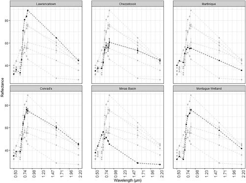
Table 2. Sentinel-2 10 and 20 m bands, with bandwidth and band center.

Band Name	Bandwidth (nm)	Band Center (nm)
B2 – Blue	66	492.4
B3 – Green	36	559.8
B4 – Red	31	664.6
B5 – Vegetation red edge	15	704.1
B6 – Vegetation red edge	15	740.5
B7 – Vegetation red edge	20	782.8
B8 – NIR	106	832.8
B8A – Narrow NIR	21	864.7
B11 – SWIR	91	1613.7
B12 - SWIR	175	2202.4

All bands were resampled to 20 m for analysis. Values are shown for Sentinel-2A for simplicity – Sentinel-2B has very similar band values.

Some similarities can be observed among the non-tailings spectra. All but the Minas Basin show absorption in the red band (B4, around 665 nm), before increasing in reflectance until around the NIR region (B8 and B8A, around 750 nm) and then steadily declining throughout the SWIR range. The red band absorption is likely due to vegetation, which was present in all sample areas except the Minas Basin despite attempting to mask it out. This same spectral shape is observed in the forest spectrum (Figure 7, top center). The spectra of Lawrencetown, Conrad’s, and the Montague wetland all match the forest spectra almost exactly, though the red band absorption is not quite as deep. This suggests a significant amount of vegetation was not successfully removed by the NDVI mask.

Figure 7. An array of biplots showing the mean spectrum for six land cover types found around the Montague mine district. Each box shows one spectrum with the other spectra in light grey for comparison. The x value of points indicates the central wavelength of Sentinel-2 bands. Whiskers around points indicate the standard error at that band. Similar spectra, at least for a certain wavelength range, were more likely to be confused when classifying. Tailings and shorelines were the most often confused classes. Absorption at Band 4 (third point from left) indicates potential chlorophyll absorption resulting from vegetation within pixels.

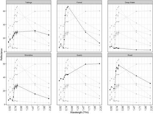
The tailings spectrum (Figure 7, top left) shows a gradual increase in reflectance between the visible and NIR bands, followed by a fairly flat response for the SWIR bands. The depth of absorption at B8 is less than the standard error, and the mean value for B8A shows no absorption at all. Martinique, Minas Basin, and Chezzetcook show similar degrees of absorption at B8, though Chezzetcook has a high standard error, possibly owing to a small sample size.

The Minas Basin reflectance increases sharply until the red edge (around 700 nm), where there is an absorption feature at B6 (740 nm), followed by a decrease throughout the NIR and SWIR region.

Results and discussion

The classifier produced positive classifications of tailings pixels at several coastal and wetland areas that upon analysis did not appear to contain tailings. Sulfide minerals were uncommon at all observed sites, including in the two Montague samples collected less than two km from the main Montague tailings area. When they were present, sulfides did not exhibit the Fe oxide or hydroxide alteration rims or remineralization that is common for sulfides found in tailings (Jewell 2021).

After confirming that the false positive areas do not contain tailings, the spectra of these areas were compared to determine the sources of confusion for the classifier. Random forest classifiers calculate the importance of each input variable during the training stage and use these importance measures in their decisions (Jewell 2024; Gregorutti, Michel, and Saint-Pierre 2017). The classifier sets some of its training points aside (an out-of-bag sample) and uses the remaining points to try and describe the subset. If all training points contain the same bias or error, that error will be included in the classifier.

An additional optimization step was included to choose an ideal set of variables (Jewell 2024). We started with the Sentinel-2 20 m bands, except for B8, and the NDVI and MNDWI indexes. The model provided 10 unique variable sets, which we tested and ranked according to F1-Score. Out of these variable sets, only four included the red band, B4, which we are considering diagnostic of vegetation. The optimization step was performed using the Goldenville and Montague mine districts, which have relatively large and unvegetated tailings areas compared to many of the other districts. Tailings in those districts were less likely to contain vegetated pixels, and less likely to have pixels with a mixed forest signal from the tailings’ edge. While the red band may not be important for defining pure tailings pixels, it is important in discriminating vegetated tailings from non-vegetated tailings. This highlights the fact that the classifier relies on more than simple iron absorption when making decisions.

Sentinel-2 has two NIR bands that overlap significantly. The narrow NIR band, B8A, is completely within the range of B8. Having multiple bands detecting the same wavelengths would be redundant and was expected to introduce bias in the classifier’s training dataset. When training the classifier, B8 was removed and the narrower B8A was kept, as it seemed easier to interpret and was thought to better target the iron absorption feature. By observing tailings spectra at multiple sites, it can be observed that absorption is negligible in B8A, but a slight absorption is often visible in B8. This suggests that iron absorption is taking place in the area of B8 that does not overlap B8A, i.e., from 800 to 853 nm.

Figure 7 shows tailings and non-tailings land cover types found around the Montague Gold Mine District. At a resolution of 20 m, a pixel will contain some combination of these land cover types, and some were more likely to produce false positive tailings classification than others. Shorelines, in particular, were prone to misclassification, as seen in Figures 4A and 4B. To determine the cause of the error and improve future results, the spectra of shorelines was compared to that of tailings, however these features were too small to eliminate pixel mixing. Coastal shorelines are larger than lake and river shorelines and provide purer pixels. They also contain similar mineralogy as they are from the same bedrock. Finally, the mean spectra of these coastal shorelines was obtained for comparison. Additionally, the mean spectra from a tidal region of the Minas Basin was recorded to represent red beds - sediment containing iron oxides that will exhibit iron absorption. Physical sampling showed that these sites do not contain tailings. Future work should be conducted to determine the results of running a classifier at these same sites to see whether they are falsely classified as tailings. Such a study could use that information to start to determine thresholds of predictability for tailings using this method.

Acknowledgments

The author would like to thank Ernie Hennick and his colleagues at the Nova Scotia Department of Natural Resources and Renewables, who produced the Nova Scotia Mine Tailings Database.

Disclosure statement

No conflict of interest was reported by the author(s).

Additional information

Funding

This research was funded by Natural Resources Canada’s Earth Observation for Cumulative Effects Program, via the Research Affiliate Program, an NSERC Discovery Development Grant [NSERC 2017 00036] and EcoCanada Student Work-Integrated Learning Program grant provided to Dr. Linda Campbell, and the Hewitt Foundation.

References

- Bates, J. L. E. 1987. Gold in Nova Scotia, Canadian Cataloguing in Publication Data. Halifax: Nova Scotia Department of Mines and Energy.
- CCME, 1997. “Canadian soil quality guidelines for the protection of environmental and human health - arsenic (inorganic).” Canadian Environmental Quality Guidelines, 7 pages.
- Clark, A.J., Labaj, A.L., Smol, J.P., Campbell, L.M., and Kurek, J. 2021. “Arsenic and mercury contamination and complex aquatic bioindicator responses to historical gold mining and modern watershed stressors in urban Nova Scotia, Canada.” The Science of the Total Environment, Vol. 787: pp. 1. doi:10.1016/j.scitotenv.2021.147374.
- Clark, R.N., and Roush, T.L. 1984. “Reflectance spectroscopy: Quantitative analysis techniques for remote sensing applications.” Journal of Geophysical Research: Solid Earth, Vol. 89 (NO. B7): pp. 6329–17. doi:10.1029/JB089iB07p06329.
- Clark, R.N., Swayze, G.A., Livo, K.E., Kokaly, R.F., Sutley, S.J., Dalton, J.B., McDougal, R.R., and Gent, C.A. 2003. “Imaging spectroscopy: Earth and planetary remote sensing with the USGS Tetracorder and expert systems.” Journal of Geophysical Research: Planets, Vol. 108 (NO. E12): pp. 5131. doi:10.1029/2002JE001847.
- Cleaver, A.E., Jamieson, H.E., Rickwood, C.J., and Huntsman, P. 2021. “Tailings dust characterization and impacts on surface water chemistry at an abandoned Zn-Pb-Cu-Au-Ag deposit.” Applied Geochemistry, Vol. 128: pp. 104927. doi:10.1016/j.apgeochem.2021.104927.
- DeSisto, S.L., Jamieson, H.E., and Parsons, M.B. 2017. “Arsenic mobility in weathered gold mine tailings under a low-organic soil cover.” Environmental Earth Sciences, Vol. 76 (No. 22): pp. 773. doi:10.1007/s12665-017-7041-7.
- DeSisto, S.L., Jamieson, H.E., and Parsons, M.B. 2016. “Subsurface variations in arsenic mineralogy and geochemistry following long-term weathering of gold mine tailings.” Applied Geochemistry, Vol. 73: pp. 81–97. doi:10.1016/j.apgeochem.2016.07.013.
- DeSisto, S.L., Jamieson, H.E., and Parsons, M.B. 2011. “Influence of hardpan layers on arsenic mobility in historical gold mine tailings.” Applied Geochemistry, Vol. 26 (No. 12): pp. 2004–2018. doi:10.1016/j.apgeochem.2011.06.030.
- Díaz-Uriarte, R., and Alvarez de Andrés, S. 2006. “Gene selection and classification of microarray data using random forest.” BMC Bioinformatics, Vol. 7 (No. 1): pp. 3. doi:10.1186/1471-2105-7-3.
- Drage, J. 2015. Review of the Environmental Impacts of Historical Gold Mine Tailings in Nova Scotia. Open File Rep. ME 2015-004 15. Halifax, Canada: Nova Scotia Geoscience and Mines Branch.
- European Space Agency 2015. Sentinel-2 User Handbook 64. Paris, France: European Space Agency.
- Goetz, A.F.H., Curtiss, B., and Shiley, D.A. 2009. “Rapid gangue mineral concentration measurement over conveyors by NIR reflectance spectroscopy.” Minerals Engineering, Vol. 22 (No. 5): pp. 490–499. doi:10.1016/j.mineng.2008.12.013.
- Gorelick, N., Hancher, M., Dixon, M., Ilyushchenko, S., Thau, D., and Moore, R. 2017. “Google Earth Engine: Planetary-scale geospatial analysis for everyone.” Remote Sensing of Environment, Vol. 202: pp. 18–27. doi:10.1016/j.rse.2017.06.031.
- Gregorutti, B., Michel, B., and Saint-Pierre, P. 2017. “Correlation and variable importance in random forests.” Statistics and Computing, Vol. 27 (No. 3): pp. 659–678. doi:10.1007/s11222-016-9646-1.
- Groves, D.I., Goldfarb, R.J., Gebre-Mariam, M., Hagemann, S.G., and Robert, F. 1998. “Orogenic gold deposits: A proposed classification in the context of their crustal distribution and relationship to other gold deposit types.” Ore Geology Reviews., Vol. 13 (No. 1–5): pp. 7–27. doi:10.1016/S0169-1368(97)00012-7.
- Guha, A. 2020. Mineral exploration using hyperspectral data. In: Hyperspectral Remote Sensing, Earth Observation, edited by P. C. Pandey, P. K. Srivastava, H. Balzter, B. Bhattacharya and G. P. Petropoulos. Hyderabad, India: Elsevier, pp. 293–318. doi:10.1016/B978-0-08-102894-0.00012-7.
- Hartlen, J. 1988. Gold! The Wealth of Waverley. Hantsport, Nova Scotia, Canada: Lancelot Press.
- Hennick, E. W., and Poole, J. C. 2020. Nova Scotia mine tailings database. Digital Product ME 533. Halifax, Canada: Nova Scotia Department of Energy and Mines.
- Hindmarsh, J., McLetchle, O. R., Heffernan, L., Hayne, O., Ellenberger, H. A., Mccurdy, R., and Thiébaux, H. J. 1977. “Electromyographic abnormalities in chronic environmental arsenicalism.” Journal of Analytical Toxicology, Vol. 1: pp. 270–276. doi:10.1093/jat/1.6.270.
- Intrinsik Corp, EcoMetrix, Crippen Berger, K., and Wood. 2019. Conceptual Closure Study for the Historic Montague Mines Tailings Areas. Final Report (Consulting). Sydney, Nova Scotia: NS Lands Inc.
- Intrinsik Corp, EcoMetrix, Crippen Berger, K., and Wood. 2020. Human Health Risk Assessment of Sediment, Surface Water, and Fish from Barry’s Run, Halifax Regional Municipality. Sydney, Canada: NS Lands Inc.
- Jewell, D. A. 2021. “Tailings classification NS repository”, Aug 22, 2023. https://github.com/djewell11/TailingsClassificationNS, doi:10.5281/zenodo.8273117.
- Jewell, D. A. 2024. Pixelwise and Object-Based Detection of Mine Tailings Using Multispectral Sentinel-2 Images.
- Koch, I., McPherson, K., Smith, P., Easton, L., Doe, K.G., and Reimer, K.J. 2007. “Arsenic bioaccessibility and speciation in clams and seaweed from a contaminated marine environment.” Marine Pollution Bulletin, Vol. 54 (No. 5): pp. 586–594. doi:10.1016/j.marpolbul.2006.12.004.
- Lane, P.A., Pett, R.J., Crowell, M.J., MacKinnon, D.S., and Graves, M.C. 1989. “Further studies on the distribution and fate of arsenic and mercury at a site contaminated by abandoned gold mine tailings.” CANMET special publication, Vol. 89–9: pp. 77–107.
- LeBlanc, M.E., Parsons, M.B., Chapman, E.E.V., and Campbell, L.M. 2020. “Review of ecological mercury and arsenic bioaccumulation within historical gold mining districts of Nova Scotia.” Environmental Reviews, Vol. 28 (No. 2): pp. 187–198. doi:10.1139/er-2019-0042.
- Mudroch, A., and Clair, T.A. 1986. “Transport of arsenic and mercury from gold mining activities through an aquatic system.” Science of the Total Environment, Vol. 57: pp. 205–216. doi:10.1016/0048-9697(86)90024-0.
- Ngole-Jeme, V.M., and Fantke, P. 2017. “Ecological and human health risks associated with abandoned gold mine tailings contaminated soil.” Plos One, Vol. 12 (No. 2): pp. e0172517. doi:10.1371/journal.pone.0172517.
- Parsons, M. B., LeBlanc, K. W. G., Hall, G. E. M., Sangster, A. L., Vaive, J. E., and Pelchat, P. 2012. “Environmental geochemistry of tailings, sediments and surface waters collected from 14 historical gold mining districts in Nova Scotia”. Halifax, Canada: Geological Survey of Canada, Open File 7150. doi:10.4095/291923.
- Parsons, M.B., and Little, M.E. 2015. “Establishing geochemical baselines in forest soils for environmental risk assessment in the Montague and Goldenville gold districts, Nova Scotia, Canada.” Atlantic Geology, Vol. 51 (No. 1): pp. 364. doi:10.4138/atlgeol.2015.017.
- Sangster, A. L., Smith, P. K., and Goodfellow, W. D. 2007. Metallogenic Summary of the Meguma Gold Deposits, Nova Scotia (Special Publication No. 5), Mineral Deposits of Canada: A Synthesis of Major Deposit-Types, District Metallogeny, the Evolution of Geological Provinces, and Exploration Methods. Nova Scotia: Geological Association of Canada.
- van der Meer, F. 2004. “Analysis of spectral absorption features in hyperspectral imagery.” International Journal of Applied Earth Observation and Geoinformation, Vol. 5 (No. 1): pp. 55–68. doi:10.1016/j.jag.2003.09.001.
- van der Meer, F.D., van der Werff, H.M.A., and van Ruitenbeek, F.J.A. 2014. “Potential of ESA’s Sentinel-2 for geological applications.” Remote Sensing of Environment, Vol. 148: pp. 124–133. doi:10.1016/j.rse.2014.03.022.
- Van der Werff, H., and Van der Meer, F. 2015. “Sentinel-2 for Mapping Iron Absorption Feature Parameters.” Remote Sensing, Vol. 7 (No. 10): pp. 12635–12653. doi:10.3390/rs71012635.
- Van Rijsbergen, C. J. 1979. Information retrieval. 2nd ed. London; Boston: Butterworths.
- Walker, S.R., Parsons, M.B., Jamieson, H.E., and Lanzirotti, A. 2009. “Arsenic mineralogy of near-surface tailings and soils: influences on arsenic mobility and bioaccessibility in the nova scotia gold mining districts.” Canadian Mineralogist, Vol. 47 (No. 3): pp. 533–556. doi:10.3749/canmin.47.3.533.
- Wilkin, R.T., and Barnes, H.L. 1997. “Formation processes of framboidal pyrite.” Geochimica et Cosmochimica Acta, Vol. 61 (No. 2): pp. 323–339. doi:10.1016/S0016-7037(96)00320-1.