Random Forest Development and Modeling of Gross Primary Productivity in the Hudson Bay Lowlands

Abstract

Peatlands are a critical component of the global carbon cycle. Within Canada, the Hudson Bay Lowlands (HBL) has accumulated an estimated 33 Gt of carbon as peat because of a small but persistent difference between gross primary productivity (GPP) and ecosystem respiration over millennia. However, the impacts of disturbance and climate change on GPP are difficult to monitor across the HBL due to its vast size and remote location. This study evaluates the potential for random forest regression models to estimate GPP at five HBL eddy covariance flux monitoring sites using only optical data from MODIS (500 m, 8 day) or harmonized Landsat/Sentinel (HLS; 30 m, 16 day or more frequent). The results show that spatial resolution has less impact on modeled daily GPP compared to temporal resolution across model configurations. Using MODIS data, individual sites’ daily GPP could be simulated with minimal bias, R² up to 0.89 and mean absolute error as low as 0.37 g C m⁻²day⁻¹. For annual GPP, MODIS (R² = 0.84; mean absolute error 40.5 g C m⁻² year⁻¹) also outperformed the HLS models (R² = 0.46; mean absolute error 86.4 g C m⁻² year⁻¹).

RÉSUMÉ

Les tourbières sont une composante essentielle du cycle du carbone. Au Canada, les basses terres de la baie d’Hudson (HBL) ont accumulé environ 33 Gt de carbone sous forme de tourbe en raison d’une différence légère, mais persistante entre la productivité primaire brute (GPP) et la respiration des écosystèmes au fil des millénaires. Cependant, les impacts des perturbations et du changement climatique sur la GPP sont difficiles à quantifier sur l’ensemble des HBL en raison de la vaste étendue du territoire et de son éloignement. Cette étude évalue le potentiel des modèles de régression de forêt aléatoire pour estimer la GPP sur cinq sites dans les HBL équipés de tour à covariance des turbulences, en utilisant uniquement les données optiques de MODIS (500 m, 8 jours) ou les données Landsat/Sentinel-2 harmonisées (HLS; 30 m, 16 jours ou plus fréquents). Les résultats montrent que dans toutes les configurations de modèle, la résolution spatiale a moins d’impact sur la GPP journalière modélisé que la résolution temporelle. À l’aide des données MODIS, la GPP journalière de chaque site a pu être simulé avec un faible biais, un R² jusqu’à 0.89 et une erreur absolue moyenne aussi faible que 0.37 g C m⁻² jour⁻¹. Pour la GPP annuelle, MODIS (R² = 0.84; erreur absolue moyenne 40.5 g C m⁻² an⁻¹) a également surperformé les modèles issus des données HLS (R² = 0.46; erreur absolue moyenne 86.4 g C m⁻² an⁻¹).

Introduction

Peatlands provide a global carbon sink that may be jeopardized by climate change and other disturbances. One of the largest contiguous peatland regions in the world is the Hudson Bay Lowlands (HBL). Here, fens and bogs account for approximately 60% of the 325,000 km² area of the HBL and store an estimated 33 Gt of carbon as peat (Martini 2006), about 25% of the Canadian peatland carbon pool (McLaughlin and Webster 2014). These ecosystems have sequestered atmospheric carbon dioxide (CO₂) over millennia through a small but persistent imbalance between carbon uptake by gross primary productivity (GPP) and carbon loss through respiration and decomposition processes (ecosystem respiration, ER).

As the climate changes, it becomes increasingly important to improve our understanding of how the HBL’s GPP may change and impact the region’s ability to absorb atmospheric CO₂ and mitigate increasing concentrations of greenhouse gases in the atmosphere (McLaughlin and Webster 2014). For example, extended growing seasons and CO₂ fertilization effects may stimulate plant growth while drying and/or permafrost degradation may give rise to soil moisture stress and reduce plant productivity (McLaughlin and Webster 2014). Industrial development and fire disturbances can also dramatically change the amount of photosynthesizing vegetation on the landscape. One method to monitor GPP in-situ at the ecosystem scale is the eddy covariance technique. This technique measures the net ecosystem CO₂ exchange (NEE) between the surface and the atmosphere, which can be partitioned to its two component fluxes, GPP and ER (Baldocchi 2003). Eddy covariance towers have been used to monitor NEE at three HBL sites since 2010, with two additional sites added in 2016 and 2017. These EC towers have provided an excellent temporal and site‑specific understanding of atmospheric CO₂ exchange processes (e.g. Helbig et al. 2019; Humphreys et al. 2014) and due to the broad coverage of peatland types and climate zones within the HBL, the data from these five sites is ideally suited for developing upscaling methods for the broader HBL.

Remotely sensed data provides the necessary scale and resolution to support classification and monitoring of vast peatlands such as those of the HBL (Lees et al. 2018). Various remote sensing platforms, including unmanned aerial vehicles, aircraft, and satellites, have been used to map wetlands (Dingle Robertson et al. 2015; Dubeau et al. 2017; Harken and Sugumaran 2005; Jensen et al. 2011; Mahdavi et al. 2018; Ozesmi and Bauer 2002) including portions of the HBL (Brook and Kenkel 2002; Franklin et al. 2018). Fewer studies however have evaluated remote sensing‑based estimates of peatland carbon fluxes. These studies have used existing GPP products (MOD17) based on Light Use Efficiency (LUE) models as well as various vegetation indices‑based models. For example, Schubert et al. (2010) used the MODIS 16‑day vegetation index composite (MOD13Q1; 16 days at 250 m) to model 16-day average GPP within the Fäjemyr and Degerö Stormyr wetlands in Sweden and concluded that strong relationships between GPP and modeled photosynthetic flux density were possible though expressed concerns with the coarse resolution of MODIS especially for smaller peatlands. Landsat (∼16 days at 30 m) data was used at two freshwater marshes in the southern Unites States (Knox et al. 2017) and successfully simulated daily GPP (R² = 0.88) though the authors highlighted issues related to heterogeneity within the Landsat pixels. Kross et al. (2013) found that a MODIS Normalized Difference Vegetation Index (NDVI) driven light use model could explain 39 to 71% of the variability of daily and annual GPP at four northern peatland sites. While over the same sites, MODIS GPP (MOD17A2) underestimated GPP at three of the four sites. Kross et al. (2013) suggested it was due to the unsuitability of the epsilon max parameter (the maximum light use efficiency under ideal conditions; ɛ_max) downscaling algorithm for peatland ecosystems.

Peatland GPP varies both spatially and temporally due to varying vegetation characteristics, hydrological conditions, temperature and light conditions, among other factors (Lees et al. 2018). Models able to take in multiple remote sensing inputs that can account for these different factors may improve remote sensing-based models of GPP within peatlands. For example, optical remote sensing vegetation indices provide proxy information on plant structural characteristics, physiological function and water stress response (Lees et al. 2018). Machine learning algorithms (MLA; e.g. random forest regression; Breiman 2001) can be used to combine multiple remote sensing data streams to estimate GPP (Tramontana et al. 2016). However, there is limited testing of these methods’ suitability for diverse peatlands such as those of the HBL. Previous MLA studies have instead focused on forest ecosystems (Chen et al. 2019), agriculture (Wolanin et al. 2019) or for the development of global estimates of GPP (Jung et al. 2020; Tramontana et al. 2016; Wei et al. 2017). Further, many MLA studies include supplemental data in the model such as climate reanalysis or land cover products (e.g. Jung et al. 2020). These data sources may help refine estimates but can also introduce additional uncertainties and errors into the model, which may be a particular concern in data-sparse regions (Bao and Zhang 2019).

Development of MLAs for carbon flux modeling requires sufficient training data which often spans multiple years and sites. A key advantage of using temporally harmonized satellite‑based RS data streams to develop models of peatland GPP such as MODIS and Harmonized Landsat Sentinel (HLS; Claverie et al. 2018) is the reduced concern about temporal and spatial artifacts due to sensor differences over the satellite era (Lees et al. 2018). However, few studies have examined the trade‑off between high temporal resolution vs. coarse spatial resolution in peatlands despite its importance.

The overall objective of this study is to determine the necessary spatial and temporal resolution and optical remote sensing variables needed to produce machine learning‑based estimations of seasonal, annual, and interannual GPP for the heterogeneous peatlands of the HBL. To accomplish this, we quantify differences in daily and annual GPP among five field sites in the HBL using EC‑derived GPP to highlight the potential heterogeneity in peatland GPP within the HBL. We then evaluate random forest regressions trained to predict GPP driven solely by HLS imagery at 30 m through 500 m pixels via downsampling. In addition, we consider differences between random forest regressions trained to predict GPP using downsampled imagery at 500 m pixels (HLS) and natively collected imagery (MODIS 8 Surface reflectance composite; MOD09A1) at 500 m pixels. Results from this study are important to improve our understanding of how sensor choice impacts the potential to model temporal and spatial patterns of GPP using MLAs in the HBL.

Data

Study site and ground measurements

The HBL is a vast peatland region located in Canada between 49° and 59° N latitude and 76° and 95° W longitude (Figure 1; Riley 2011). Permafrost is continuous at the northern edges of the HBL and becomes increasingly sporadic toward the south with only seasonal frost at its southern tip (Riley 2011). Peat depth increases from north to south in both the fens and bogs. Fens and bogs cover the majority of the HBL (60%). In contrast, peat plateaus, palsa, tundra, woodland, forest and swamp cover ∼27% of the HBL (Riley 2011), with peat plateaus found solely in the northern portions of the HBL within the continuous permafrost zone. The remaining 13% is classified as open water, marshes, or barren rock and burned areas (Riley 2011).

Figure 1. The Hudson Bay Lowlands ecozone is outlined in blue. The eddy covariance flux tower research sites are marked in yellow. The base map is provided by Esri.

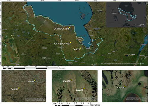
The five HBL EC flux towers are situated within different peatland types (Figure 1) as part of an ongoing research program to monitor peatland carbon flux between the surface and the atmosphere. These sites differ in their characteristics, including peat characteristics and depth, permafrost, vegetation and climate (Table 1). The EC and meteorological instrumentation at each site is as follows: an HS‑50 sonic anemometer (CA‑ARB, CA‑ARF, CA‑KLP; Gill Instruments, Lymington, England) or a CSAT3B sonic anemometer (CA‑PB1 and CA‑PB2; Campbell Scientific Inc., Logan, UT; CSI) measures 3‑dimension wind velocity, an enclosed infrared CO₂/H₂O gas analyzer (LI‑7200, LI‑COR, Lincoln, NE; LI-COR) measures CO₂ and H₂O mixing ratios, an aspirated and shielded HMP45C sensor (CSI) ∼4 m above the surface measures air temperature and relative humidity, a LI‑190SB quantum sensor (LI‑COR) measures photosynthetically active radiation, and a Kipp and Zonen CNR4 (OTT HydroMet Corp, Sterling, VA) measures 4‑component (upwelling and downwelling shortwave and longwave) radiation.

Table 1. Overview of the site characteristics for the five eddy covariance (EC) tower sites in the Hudson Bay Lowlands. The Site ID is the site designation associated with the Ameriflux database (www. ameriflux.lbl.gov).

Site ID	CA-PB1	CA-PB2	CA-ARB	CA-ARF	CA-KLP
Site name	Polar Bear Provincial Park 1	Polar Bear Provincial Park 2	Attawapiskat River Bog*	Attawapiskat River Fen*	Kinoje Lake Peatland^†
Latitude, longitude	54.941° N, 83.457° W	54.939° N, 83.473° W	52.695° N, 83.945° W	52.700° N, 83.955° W	51.590° N, 81.768° W
EC flux measurement height	3.5 m	3.5 m	7.5 m	7.5 m	3 m
Common vegetation	Lichens, ericaceous shrubs	Sedges, Sphagnum spp., sparse black spruce and larch trees	Sphagnum spp., lichens, ericaceous shrubs, cotton grass, black spruce trees	Sphagnum spp., scorpion tail moss, wire sedge, buckbean, marsh horsetail, larch trees	Sphagnum spp., lichens, ericaceous shrubs
Site description	Lichen dominated peat plateaus underlain by permafrost interspersed with thawed sedge dominated lawns	Ephemeral peat pools and sedge lawns with elevated margins populated by with ericaceous shrubs and stunted trees	Hummock/hollow bog with scattered trees, few pools	Patterned fen with treed ridges and sedge lawns	Shrub‑dominated bog, small and sparse black spruce and tamarack trees
Peat depth	0.4–2 m (Riley 2011)	0.4–2 m (Riley 2011)	2 m (Humphreys et al. 2014)	2 m (Harris, 2017)	1.4–2.7 m (Klinger et al., 1994)
Mean annual air temperature (°C)^‡	-2.9	–2.9	–1.1	–1.1	–0.2
Average annual precipitation (mm)^‡	476	476	544	544	668
Measurement years (number of years used to calculate annual GPP)	2016–2019 (3)	2017–2019 (2)	2011–2019 (5)	2011–2019 (9)	2011–2019 (6)
Average annual GPP ±1 standard error (g C m^-2 year^-1) and annual coefficient of variation (CV)	153 ± 17 (0.19)	199 ± 16 (0.13)	365 ± 10 (0.06)	462 ± 14 (0.09)	314 ± 7 (0.05)

*See Helbig et al. (2019) for more site details.

^†See Humphreys et al. (2014) for more site details.

^‡Prairie Climate Center (2019).

Remote sensing data

Landsat 7 and the Harmonized Landsat‑Sentinel (HLS) database (Claverie et al. 2018) provided 30 m resolution imagery in six spectral bands and the MODIS 8‑day surface reflectance composite (MOD09A1) provided 500 m resolution imagery over the sites between 2011–2019.

To fill in the gaps in Landsat 7 data caused by the scan line corrector instrument failure, the missing data was interpolated based on the method described by Zhu et al. (2012) based on a single image. Briefly, this method first classified the base image into broad classes. The data was then detrended in each of these classes using an empirical model between the base and target images. A semivariogram was calculated based on the residual for each class. The residual of the unscanned pixel was found through kriging on a sample of nearby pixels in the same class from the base image. The final prediction was the result of adding the trend back in. Two Landsat 7 images were used, and any gaps remaining from where neither image scanned were filled with no data. Where possible, the pair of images corrected each other, each acting as the base and target image.

To harmonize the Landsat 7 images with the HLS data, the Landsat 7 images were cross‑calibrated to the HLS database through band to band linear regression (Tokola et al. 1999). To develop the regression, Landsat 7 images were paired with images from the HLS data that were at most one day apart, and a sample was taken every 100 pixels from the 4 km region surrounding the tower. This resulted in 56 images and 8258 pixels for each band. The samples were taken before the correction for the scan line correction was applied so that no interpolated values were present in the regression samples. The pixels were considered to be pseudo-invariant due to the small time difference between pairs while the large number of pixels used in this process ensured the regression was not susceptible to outliers. This image processing was carried out in PCI Geomatica (v. Banff, Catalyst).

Processing

The EC measurements were processed following a standard procedure using EddyPro v. 7.0.6 (LI‑COR) for each site. Fluxes were computed at 30‑minute intervals using block averaging, double coordinate rotation, compensation of time lags between vertical velocity and CO₂/H₂O mixing ratios by covariance maximization, and analytical correction of high‑ and low‑pass filtering effects (Moncrieff et al. 2004; Moncrieff et al. 1997). NEE was calculated as the sum of the 30 min CO₂ flux and the rate of change in storage of CO₂ below the height of the EC instrumentation using CO₂ measured at EC height (Table 1). 30 min NEE was used to derive the two component fluxes, GPP and ER. NEE is negative when there is net CO₂ uptake by the ecosystem. Derived GPP is positive when there is photosynthetic uptake of CO₂ by the vegetation and measured or modeled ER is positive when there is CO₂ emission from the ecosystem to the atmosphere.

A standard quality assurance protocol was applied to all sites’ NEE fluxes. This included removing low‑quality data points as determined using reasonable vertical velocity and temperature statistical thresholds, friction velocity thresholds and removal of fluxes exceeding three standard deviations from the mean of a 30‑day window period (see Humphreys et al. 2014 for further details). Ancillary measurements such as 4-component radiation, air temperature, relative humidity and photosynthetic photon flux density occasionally were missing observations, normally only due to power or instrument failure. Where present, these gaps were gap-filled using ERA5 reanalysis data (Hersbach et al. 2020) adjusted to site observations using a linear regression over a 5-day moving window.

The NEE data was decomposed into GPP and ER based on a method described by Reichstein et al. (2005). Nighttime NEE (equivalent to ER) measured when friction velocity > 0.1 m s^‑1 was used to determine a Q₁₀ relationship between all ER and air temperature for a given site. ER was then estimated for daytime half hours and any missing nighttime half hours using this relationship adjusted by a short‑term temperature sensitivity parameter calculated using the nearest 200 half hours of observed ER. GPP was then calculated as the difference between modeled ER and measured NEE.

A light response model (see for example, Humphreys et al. 2014) was used to gap‑fill GPP when solar radiation was greater than 25 W m^‑2; otherwise, GPP was set to zero. The two model parameters, A_max, the maximum photosynthetic uptake rate of CO_2, and α, effective quantum yield, were derived using 30 min values of GPP and photosynthetic flux density limited to July and August each year. The modeled GPP was then adjusted to observations to account for phenological and environmental conditions by applying a multiplier determined from a regression between modeled and measured values within a 200 half hour window moved in increments of 40 half hours. GPP was then aggregated to daily sums (g C m^‑2day^‑1).

This partitioning/gap‑filling method for GPP performed poorly for periods with few NEE measurements as there was no plant phenology information included in the model. To account for this, daily GPP values were excluded for any month with less than 25% observations. Annual GPP values were also not presented for years with missing growing season months (March through September).

An alternative gap filling method was applied to the GPP data using a neural network method as different gap-filling methods can impact daily and annual GPP values (e.g. Moffat et al. 2007). Annual sums from the two gap-filling methods were compared to assess how these data processing procedures impacted study results. The neural network filled the GPP gaps in three stages. First nighttime GPP values were filled with zeroes, then small gaps (one half‑hour) were filled using linear regression based on the two adjacent values. The third stage used a neural network to fill the gaps based on similar data points in the time series. The network was trained to predict GPP using only auxiliary weather variables measured at each site (relative humidity, air temperature, shortwave radiation upwelling and downwelling), the number of days away from an expected peak in GPP (July 20) and the average GPP of all years for each date. Any remaining gaps were then linearly interpolated. The two gap‑filling methods agreed well when there were NEE measurements near the gap periods to ground the estimates, while substantial differences between the two gap‑filling methods occurred when there were few observations.

Differences in GPP among sites and years were examined through the Jeffries‑Matusita (JM; Swain and King 1973) distance to better understand the spatial and temporal variations in GPP within the HBL. A moving window of 15 days was used to calculate the JM distance for each day throughout the growing season between the day of year (DOY) 120 and 300. This excluded near‑zero GPP below the noise threshold for the system when no or limited photosynthesis was expected. A JM distance threshold of 1.7 indicated there was significant separability between GPP for 15-day window periods among sites (intersite variability) and within sites (intrasite variability).

Modeling

Eighty‑five optical remote sensing variables were initially considered for random forest regression to represent daily GPP (Appendix 1). These included 37 vegetation indices selected to highlight different biophysical and biochemical parameters on the ground. These vegetation indices are typically used for mapping and monitoring parameters such as leaf area index, chlorophyll content, water content, biomass, senescence, and pigment concentrations (Gitelson et al. 2003; Haboudane et al. 2004). In addition, eight omnidirectional gray level co‑occurrence measures of texture were calculated across two different window sizes (3 and 15 pixels) with a lag of one pixel for each band. Initial comparisons indicated no substantial difference between the two window sizes, and strong correlations were present, so only a window size of 3 pixels was used in the random forest analysis. The 85 possible variables were then examined for correlations between them. Any variable with a coefficient of determination (R²) greater than 0.85 was flagged, and the variables with the highest number of correlations were removed. This process was repeated until the set of variables no longer had R² values above the 0.85 threshold. For both the HLS and MODIS datasets, 41 variables remained. To assess image spatial resolution on the random forest representation of GPP, the HLS variables were re‑calculated using downsampled images at 500 m, in addition to the native 30 m resolution.

To pair the remote sensing data and the EC data for random forest regression, the spatial mean value from the pixels surrounding the tower in a 125 m radius centered on the tower was used. This radius included at least 70% of the EC tower flux footprint, which represents the source area for the fluxes measured at the tower (Kljun et al. 2004). At all sites, the peatland characteristics were relatively homogenous for several hundred meters around the towers (Figure 1) and ensured the remote sensing imagery was reflective of the flux tower source area. Any pixel falling within this area (∼69 pixels at 30 m resolution) contributed to an unweighted mean value for that image date. The number of daily gap-filled GPP observations coincident with quality remote sensing imagery ranged from 13– 213 per year for HLS and 61–105 per year per site for MODIS (Appendix 2).

The random forest regressions were developed with 400 trees in each forest using six different groupings of the five field sites’ observations (site configurations). A “leave one out” approach was used where one year was used as validation while the remaining years were used as training data. Every year was used once as validation. Each random forest had the least important variables removed until only ten variables remained to limit the complexity of the model but maintain good performance. The permutation importance criterion was used to rank variables with respect to their contributions to a given random forest. This criterion randomly permutes a variable to disrupt its relationship with the output (Breiman 2001). The change in accuracy between the permutated and original values averaged across all trees indicates the variable importance. Relative variable importance was examined for 810 random forests (five random forests in each of the 9 available observation years; minimum, maximum and average of 7-day GPP; six site configurations).

To examine the sensitivity of the models to the training data, the random forests were developed using different GPP inputs and different sets of field sites. The minimum, maximum, and average daily GPP observed at the EC flux towers were calculated for window periods of three and seven days surrounding the image acquisition date in addition to using a single day daily GPP coincident with the image acquisition date. Random forest models were developed for six different site configurations: three individual EC sites (CA-PB1 and CA-PB2 were not used individually as there was insufficient data for model training and validation), all five sites combined, and two pairs of sites. The configurations of sites pairs included the two bog sites (CA‑ARB and CA‑KLP) and the two neighbouring sites (CA-ARB and CA-ARF) that experienced the same climate and weather controls and had multiple years of observations. In summary, 252 random forest configurations were trained: six site combinations (all five sites combined, the three individual southern sites, bogs only, and Attawapiskat River sites only) × three resolutions (HLS 30 m, HLS 500 m, MODIS 500 m) × seven EC values and window sizes pairs (daily GPP on imagery date, maximum GPP, minimum GPP, average GPP for 3 and 7-day windows around imagery date) × two NDVI thresholds (0.1 and none). To limit the influence of many near-zero values from the cold season when photosynthesis did not occur, observed NEE was small but positive and derived GPP was negligible, an NDVI threshold of 0.1 was applied to the validation data before calculating the model quality metrics. Models were assessed using R², the mean error (ME) and the mean absolute error (MAE).

To compare measured and simulated total annual GPP, EC‑derived annual GPP was calculated as the sum of the daily gap‑filled GPP values throughout the year for years with no missing growing season months. Annual GPP was calculated using the random forest regression model results based on a trapezoidal integration of the set of image dates (Appendix 2) for each year. All modeling and analyses were carried out using Matlab v.9.14 (The MathWorks Inc 2023).

Results

Spatial and temporal variability in GPP at the Hudson Bay Lowland field sites

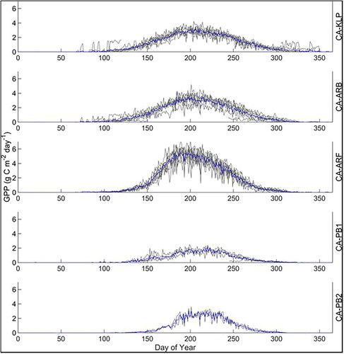
The five HBL sites demonstrated both inter and intrasite variability in GPP (Table 1, Figure 2). Average annual GPP varied from 153 to 462 g C m^‑2year^‑1 (Table 1). Of the southern sites, CA‑ARF had a greater range of daily GPP values than either of the bog sites, CA-ARB and CA-KLP (Figure 2). The northernmost sites had expectedly lower GPP values throughout the season and a shorter growing season than the southern sites (on average 133 days/year at CA‑PB1 and CA‑PB2 vs. average of 183 days/year at CA‑ARF, CA‑ARB, and CA‑KLP based on the period with GPP greater than 0.25 g C m^‑2day^‑1). The coefficient of variation (CV) for annual GPP was greater for all the sites combined (CV = 32%, n = 25) than for annual GPP for a given site (CV from 5 – 19%).

Figure 2. Ensemble average daily GPP over all measurement years (blue line) and daily GPP for each measurement year (grey line) for the five HBL EC sites between 2012 and 2019, inclusive. There are 9 of years with observations for CA‑KLP, CA‑ARB and CA‑ARF, 4 years at CA‑PB1 and 2 years at CA‑PB2.

The JM distance was used to compare GPP over 15-day periods over the growing season within and amongst the sites (Figures 3 and 4). Interannual variability of GPP over a 15-day window period was most often discernible using JM distances with a threshold of 1.7 at CA‑KLP (5.6%), CA‑ARB (6.9%), CA-PB2 (4.4%) and rarely at CA‑ARF or CA-PB1, where less than one percent of the 15‑day window periods were separable (Figure 3). The period of time during the growing season that gave rise to this interannual variability in GPP (or lack thereof) varied among sites. For example the timing of greatest intrasite JM distance separability at CA-ARF was near the end of the season when plants were senescing while CA‑PB1, CA-PB2 and CA-KLP had peak JM distances that reoccurred throughout the season (Figure 4b). These results suggested that GPP was responding to one or more environmental factors that varied throughout the season such that year-to-year differences in snowmelt timing in spring, mid-summer dryness, or late-summer/early fall temperatures may have been important factors driving interannual variability in GPP at these sites (Figure 2).

Figure 3. Percent of 15‑day moving windows between day 120 and 300 that have a Jeffries‑Matusita (JM) distance above 1.7. JM distance is calculated on daily GPP for the five eddy covariance tower sites in the HBL. Intersite comparisons use the same year while intrasite compare multiple years.

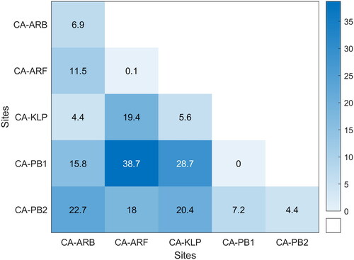
Figure 4. Average Jeffries‑Matusita (JM) distance for 15-day windows between day of year 120 and 300 using all possible pairs of sites to illustrate intersite variability (left) and using all possible pairs of site years for a given site to illustrate intrasite variability (right). JM distance is calculated on daily GPP for the five eddy covariance tower sites in the HBL.

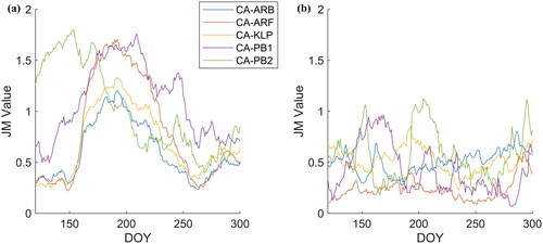
Considering separability among sites, the largest separability was between the Polar Bear sites and the more southern sites, particularly CA-PB1 and CA-ARF where nearly 39% of the 15-day average JM distances exceeded the 1.7 threshold (Figure 3). Temporally, the JM distance showed a consistent pattern for four of the five sites with the largest JM distances and thus greatest differences among sites from early June to early August (∼DOY 160‑220; Figure 4a). The JM distance rapidly climbed toward DOY 160 as GPP increased with rising air temperatures and greening vegetation. In contrast, CA-PB2 JM distance values started high from the beginning and declined through the season in part due to having the slowest spring increase in GPP of all the sites (Figure 2). Following DOY 220 in early August, CA-PB1 remained highly separable from the other sites as GPP remained relatively low on the lichen dominated permafrost plateau when compared to the other sites and senescence began earlier in the year than at the southern sites (Figure 2).

Random forest regression models of GPP

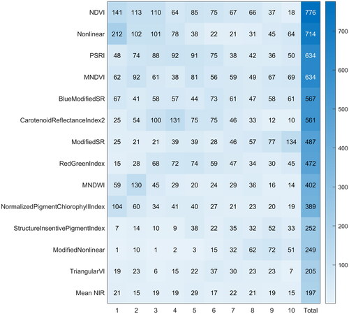
Of the 41 variables that remained in the reduced variable set following the removal of those with high correlations, all 41 appeared at least once in a random forest regression model used to predict GPP although 27 of the variables appeared in less than 20% of the 810 models considered. Figure 5 lists the 14 variables that appeared in over 20% (162) of the models. The variables which appeared most often (at any rank position) were NDVI (in 776 models or 96%), nonlinear vegetation index (714 or 88%), PSRI (634 or 78%), and Modified NDVI (634 or 78%). The nonlinear vegetation index most often appeared as the first ranked variable (in 212 models) followed by NDVI (141) and Normalized Pigment Chlorophyll Index (104). There was a degree of stratification present in the variable importance ranking. For example, NDVI and the nonlinear vegetation index were most often ranked in the top three variables within the models while Carotenoid Reflectance Index 2 was most often ranked in positions three through six and Modified Simple Ratio was most often ranked in position ten. In contrast, the ranking for Blue Modified Simple Ratio was evenly distributed through positions one through ten and was the 5^th most common variable in the models.

Figure 5. Importance ranking for the remote sensing variables included in the final set of 810 random forest regression models evaluated in this study. The rank positions are listed along the bottom axis and the number of times a given variable is ranked at that position is listed within the column. The final column indicates the number of times that variable was included within the set of 810 random forest models. Note each final individual model included only ten variables to limit their complexity. Only variables appearing in over 20% (162) forests are shown.

The random forest regression models trained to predict GPP using all five sites were not highly impacted by differences in the GPP metric (average, maximum or minimum) nor the size of window (1, 3 or 7 days centered on the date of acquisition of the imagery; Table 2). R² values were least for the 500 m HLS (0.51 to 0.62), slightly greater for the 30 m HLS (0.55 to 0.65) and greatest for the 500 m MODIS 8‑day composite (0.71 − 0.78; Table 2). There was minimal bias in the mean error for all models, and the MAE was between 0.45 and 0.75 g C m^‑2day^‑1. Note that these model evaluation metrics were computed using GPP values computed in the same manner as for the model development (e.g. 1-day mean or 3‑ or 7‑day mean, max or min) and thus the models based on maximum and minimum GPP represented highest and lowest values during the window periods, respectively. When these random forest models were used to estimate annual GPP sums, models developed using minimum or maximum GPP substantially under or overestimate the total annual GPP, respectively (not shown). For this reason and due to consistently good results across the metrics considered, the 7‑day average GPP random forest was chosen to demonstrate the effects of the remaining model selection configurations.

Table 2. Effects of different GPP statistics used with Harmonized Landsat Sentinel (HLS) 30 m, HLS 500 m and MODIS 8 Day composite remote sensing data to develop random forests for all five HBL peatland sites. An NDVI threshold of > 0.1 is applied to the validation data to limit the impact of multiple low values early in the season. The metrics without this threshold are included in brackets. Mean absolute error and mean error values are g C m^-2 day^-1.

GPP statistic	30 m HLS			500 m HLS			MODIS composite 500 m
	R^2	Mean absolute error	Mean error	R^2	Mean absolute error	Mean error	R^2	Mean absolute error	Mean error
1 Day Value	0.64 (0.68)	0.64 (0.61)	0.06 (0.08)	0.61 (0.66)	0.65 (0.63)	0.01 (0.03)	0.72 (0.77)	0.54 (0.48)	–0.02 (–0.01)
Average (3 Days)	0.63 (0.67)	0.61 (0.59)	0.05 (0.08)	0.62 (0.64)	0.63 (0.62)	0.00 (0.03)	0.77 (0.80)	0.49 (0.44)	–0.02 (–0.01)
Average (7 Days)	0.65 (0.68)	0.60 (0.58)	0.06 (0.08)	0.60 (0.64)	0.63 (0.61)	0.01 (0.03)	0.78 (0.82)	0.46 (0.43)	–0.02 (–0.01)
Maximum (3 Days)	0.64 (0.67)	0.66 (0.65)	0.05 (0.08)	0.60 (0.65)	0.69 (0.67)	0.00 (0.03)	0.77 (0.81)	0.54 (0.49)	–0.02 (0.00)
Maximum (7 Days)	0.63 (0.68)	0.72 (0.68)	0.05 (0.07)	0.57 (0.64)	0.75 (0.71)	0.00 (0.02)	0.77 (0.82)	0.56 (0.51)	–0.02 (–0.01)
Minimum (3 Days)	0.59 (0.65)	0.60 (0.56)	0.03 (0.05)	0.54 (0.60)	0.64 (0.60)	–0.01 (0.02)	0.73 (0.77)	0.49 (0.43)	–0.02 (–0.02)
Minimum (7 Days)	0.55 (0.57)	0.58 (0.55)	0.03 (0.05)	0.51 (0.57)	0.61 (0.57)	0.02 (0.03)	0.71 (0.76)	0.45 (0.40)	–0.02 (–0.01)

The random forest results varied depending on whether they were trained on individual sites, paired sites or all sites combined (Table 3). When NDVI was limited to values greater than 0.1, the models’ R² ranged from 0.52 to 0.89 with minimal bias and MAE of 0.37 to 0.90 g C m^‑2day^‑1. The three models with the greatest R² used 500 m MODIS and were for individual sites (e.g. CA-ARF: R² =0.89, MAE = 0.46 g C m^‑2day^‑1; CA-KLP: R² =0.84, MAE = 0.37 g C m^‑2day^‑1) and the two Attawapiskat sites combined (CA-ARF & CA-ARB: R² =0.80, MAE = 0.50 g C m^‑2day^‑1).

Table 3. Effects on the random forest quality for different site groupings using Harmonized Landsat Sentinel (HLS) 30 m, HLS 500 m and MODIS 8‑day composite remote sensing data for ten variable random forests. A 7‑day average GPP is used for these models. An NDVI threshold of >0.1 is applied to the validation data to limit the impact of multiple low values early in the season. The metrics without this threshold are included in brackets. Mean absolute error and mean error values are g C m^-2 day^-1.

Site groups	30 m HLS			500 m HLS			MODIS composite 500 m
	R^2	Mean absolute error	Mean error	R^2	Mean absolute error	Mean error	R^2	Mean absolute error	Mean error
ALL	0.65 (0.68)	0.60 (0.58)	0.06 (0.08)	0.60 (0.64)	0.63 (0.61)	0.01 (0.03)	0.78 (0.82)	0.46 (0.43)	–0.02 (–0.01)
CA‑KLP	0.75 (0.78)	0.48 (0.50)	–0.05 (0.01)	0.63 (0.71)	0.46 (0.51)	0.02 (0.07)	0.84 (0.87)	0.37 (0.36)	–0.02 (–0.01)
CA‑ARF	0.64 (0.68)	0.79 (0.76)	0.02 (0.12)	0.64 (0.71)	0.90 (0.77)	–0.06 (0.00)	0.89 (0.89)	0.46 (0.45)	–0.02 (0.02)
CA‑ARB	0.53 (0.60)	0.59 (0.57)	–0.10 (–0.09)	0.52 (0.60)	0.60 (0.57)	–0.11 (–0.09)	0.77 (0.81)	0.46 (0.43)	–0.03 (–0.03)
CA‑KLP & CA‑ARB	0.54 (0.70)	0.51 (0.48)	–0.03 (0.00)	0.56 (0.68)	0.49 (0.50)	–0.05 (–0.01)	0.75 (0.81)	0.41 (0.38)	–0.01 (–0.01)
CA‑ARF & CA‑ARB	0.62 (0.73)	0.73 (0.64)	0.01 (0.07)	0.57 (0.73)	0.77 (0.64)	0.00 (0.07)	0.80 (0.86)	0.50 (0.42)	–0.01 (0.00)

When all five sites were combined, the 500 m MODIS model had greater R² (0.78) and least MAE (0.46 g C m^‑2day^‑1) when compared to the random forests trained with either 30 m HLS (R² =0.65, MAE = 0.60 g C m^‑2day^‑1) or 500 m HLS (R² =0.60, MAE = 0.63 g C m^‑2day^‑1). The random forests for all five sites were almost always better than the models for paired sites within a given imagery data source. Only the 500 m MODIS random forest for the two Attawapiskat sites had slightly greater R² (0.80 for two sites vs. 0.78 for five sites) though MAE was lower for the random forest for all five sites (0.46 g C m^‑2day^‑1 for five sites vs. 0.50 g C m^‑2day^‑1 for two sites).

The random forests using 30 m HLS had similar or slightly greater R² than the 500 m HLS models. At 30 m and 500 m resolution, the model with greatest R² and least MAE was for CA‑KLP alone (30 m: R² =0.75, MAE = 0.48 g C m^‑2day^‑1; 500 m: R² =0.63, MAE = 0.46 g C m^‑2day^‑1). The model improvement was less when changing how the GPP data was paired with the remote sensing data (Table 2) compared to when the number of sites was varied (Table 3). This was likely due to the increased temporal resolution due to the greater number of data points using MODIS data, especially in the early years prior to the launch of Landsat 8 and Sentinel‑2A and 2B (Appendix 2). This allowed additional points in the training set to better characterize the spatial and temporal variability in the sites’ GPP.

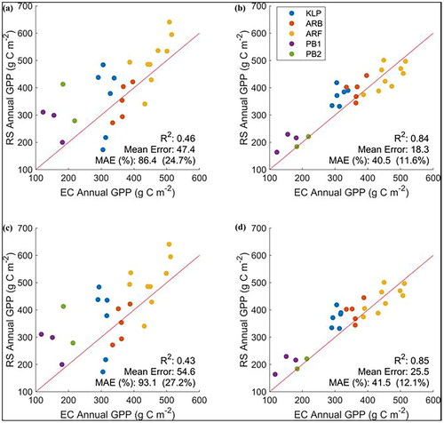
The temporal resolution of the random forest input data became even more important when annual sums of GPP were computed from the random forest estimates. The random forest model developed on all five EC sites using MODIS data consistently outperformed the HLS model when compared to annual GPP derived from EC measurements gap‑filled either with the light use efficiency method (30 m HLS R² = 0.46; Figure 6a vs. 500 m MODIS R² = 0.84; Figure 6b) or the neural network method (30 m HLS R² = 0.43; Figure 6c vs. 500 m MODIS R² = 0.85, Figure 6d). Despite limited training data for the northern CA‑PB1 and CA-PB2 sites, the models were able to distinguish among sites with greater annual GPP in the south and lower annual GPP in the north where the climate was cooler and there was less vegetation. These models simulated interannual GPP at the individual sites with less skill (Figure 6). For example, R² and MAE values for the 500 m MODIS model results compared to annual EC-derived GPP gap-filled using the light use efficiency model was 0.40 and 37.1 g C m^‑2year^‑1 at CA-ARF, 0.18 and 35.1 g C m^‑2year^‑1 at CA-ARB, and 0.14 and 58 g C m^‑2year^‑1 at CA-KLP, respectively (not shown).

Figure 6. Predicted vs measured annual GPP for a random forest regression model developed for all five sites using 7‑day average daily GPP from eddy covariance (EC) measurements and either 30 m Harmonized Landsat Sentinel data (a, c) or 500 m MODIS 8‑day composite data (b, d). EC Annual GPP is the annual GPP calculated for the flux tower sites using gap-filled GPP using the light use efficiency (a, b) and the neural network method (c, d). Mean absolute error (MAE) is given as a value (g C m⁻²year⁻¹) as well as a percent of the mean annual GPP. Years with months between April‑Nov with less than 25% observations were not included in the analysis. The red line is a one-to-one line.

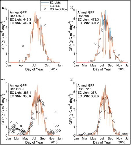
The performance of the random forests in predicting GPP was best for later years when more imagery was available (Figure 7) and tended to agree best with annual GPP gap-filled using the light response method when gaps were larger (Figure 7b). However, at some sites, such as CA‑ARF, where there was limited intrasite variability in seasonal GPP (Figures 3 and 4), a limited number of images over multiple years did quite well in representing the annual GPP compared to other sites. The trapezoidal integration used to find the annual GPP relies on a few well‑timed images throughout the time series that captures the phenological curve (Figure 7a,b). After 2017, following the launch of both Sentinal‑2A and 2B as well as Landsat 8, the image density was the same, if not higher than the MODIS data for the same year, and the capability of the random forests to track the phenological curve was improved (Figure 7c,d).

Figure 7. Comparison of remote sensing (RS) random forest regression model predictions (orange circles) using Harmonized Landsat Sentinel (HLS) data for 2012 (a), 2013 (b) and 2018 (c) and MODIS data for 2018 (d) for CA-ARF. Daily measures of gross primary productivity (GPP) derived from eddy covariance (EC) measurements are shown gap-filled by a light use efficiency model (EC Light, blue lines) and by a single neural network (EC SNN, red lines). Annual GPP (g C m⁻²) is given for the remote sensing random forest model (RS) using trapezoidal integration and for the EC measurements gap-filled using the light use efficiency method (EC Light) and the neural network method (EC SNN).

Discussion

This study highlighted the considerable spatial and temporal variability in HBL peatland GPP that has been noted in a few other studies that examined data from these specific sites (Helbig et al. 2019; Humphreys et al. 2014) and other studies in the region (Frolking et al. 1998; Whiting 1994). For example, Helbig et al. (2019) demonstrated clear differences in GPP at CA‑ARF and CA‑ARB and in the GPP response to temperature owing to differences in deciduous and evergreen vegetation between these two sites. The greatest temporal separability in GPP corresponded to mid‑growing season (Figure 4) and this agreed well with work by Helbig et al. (2019) where midseason GPP values were most important when describing the annual GPP for CA‑ARB and CA‑ARF. Kross et al. (2014) found that ‘peak CO₂ exchange rate’ was best for separating the four northern peatlands considered in their study. Other points of separability were found within the spring and fall shoulder seasons, which was mostly linked with the later onset of green‑up and earlier senescence at the more northerly sites where growing seasons were shorter (Figure 4). Thus, a successful remote sensing‑based model of GPP in the HBL must be able to represent different magnitudes of GPP during the mid growing season and shoulder seasons to represent the phenology of peatlands with different vegetation and climate.

Overall, the random forest models performed well and were in line with results from other global studies (Joiner et al. 2018; Sun et al. 2018) or regional studies (Li et al. 2013; Olofsson et al. 2008) of satellite-driven models of GPP. For example, Joiner et al. (2018) reported R² values between 0.60 and 0.75 for light use efficiency models using solar induced florescence compared with the FLUXNET dataset. Sun et al. (2018) found that solar induced florescence from the orbiting carbon observatory agreed well globally with the FLUXCOM dataset (R² = 0.6 to 0.8). Olofsson et al. (2008) found that EVI and NDVI from MODIS could track the monthly GPP values across seven sites in Northern Europe (R² = 0.7 to 0.9).

These studies frequently discussed the importance of sufficient ground data, concerns with cloud cover preventing remote sensing data acquisition, and concerns over temporal resolution of the remote sensing data. Photosynthesis at the ecosystem scale varies slowly through the season in response to seasonal changes in vegetation, temperature, moisture and light, for example. However, GPP can also change rapidly throughout the day and from day to day generally due to changing light levels. Thus, while the impact of cloud cover on satellite image acquisition can be limited through the use of composites (e.g. MODIS 8‑day), regular coverage is not guaranteed in particularly cloudy areas such as the tropics (Sun et al. 2018). In addition, this compounds the issue that the imagery taken at a single instance in time is unlikely to represent the average variability in conditions affecting GPP. For example, the HLS random forest in 2018 for CA-ARF (Figure 7c) predicted the lower GPP associated with two sudden drops in daily GPP in the mid season, however it did not correctly simulate the prior time period where GPP was greater, as is more typical at that site. Sun et al. (2018) found that none of the models they checked were exactly consistent with the ground data though results were within the confidence intervals. This agreed well with what was seen in our results; the random forests were able to represent seasonal trends better than the short‑term variability in GPP (Figure 7c,d).

In this study, we explored the impacts of different random forest model input data including varying 1) the EC‑based GPP training/validation data based on a 1‑, 3‑ and 7‑day window and different statistical metrics, 2) the sites for model development (site configuration), 3) spatial resolution of the satellite imagery, and 4) temporal resolution of satellite imagery. The factors with the greatest impact on the success of the model as determined using R², mean error and MAE were site configuration and temporal resolution. The impact of varying the EC‑based GPP statistics on the models was minimal. This finding was expected since the random forest model is purely a statistical model and does not have any predetermined assumptions about the relationships between the satellite variables and the EC‑based GPP used to train and test the model. As such, it can readily adapt to the training data and provide similar quality models to predict minimums, maximums and averages from the EC data. For both MODIS 8-day composite and HLS‑based random forest models, the results were best with the 7‑day average GPP rather than the 1-day GPP despite HLS imagery corresponding to a specific date.

This study demonstrated that the random forest algorithm was adaptable to various site configurations while some configurations were more successful than others. For example, the MODIS 8-day composite random forest model for CA‑ARF performed best out of all the models despite a greater amount of training data available for site configurations that included multiple sites. The JM distance analysis suggested that GPP at CA-ARF was not substantially different across years, and thus there appeared to be sufficient representative data to allow the algorithm to learn CA‑ARF’s phenological curve. Millard and Richardson (2015) highlighted the importance of sufficient training data as well as its representativeness in determining how accurate a random forest could be for peatland classification. Rodriguez-Galiano et al. (2012) highlighted that homogenous classes are less impacted by training set size while heterogenous classes are much more sensitive to reduced training set sizes. Nevertheless, the model for all five sites combined was able to clearly differentiate CA-ARF, CA‑PB1 and CA-PB2, which had some of the highest intersite JM distance values, despite limited training data for CA-PB1 and CA-PB2 (Figure 3).

Variable importance analysis indicates which variables hold the most explanatory power within the model and is frequently used for variable selection (Breiman 2001; Nicodemus 2011). Despite the differences in model performance among the HBL sites, variable importance analysis demonstrated that there were several variables common to 78% or more of the models: NDVI, nonlinear vegetation index, PSRI and Modified NDVI. These indexes use the near‑infrared and red bands, which have well‑documented relationships with plant abundance and productivity as healthy green, photosynthesizing plants absorb in the red and reflect in the near-infrared bands (e.g. Lees et al. 2018; Xue and Su 2017). Although NDVI and similar vegetation indices can saturate where there is high leaf area, this may be less of a concern in northern peatlands such as these and elsewhere (Lees et al. 2018). Spectral indices which make use of near-infrared water absorption is also a potentially important means to separate among peatlands (e.g. Kolari et al. 2022), particularly those with limited vascular plant cover and instead are dominated by wet Sphagnum moss and ephemeral pools (e.g. CA-PB2) or flarks (CA-ARF). PSRI also includes the green band and is associated with the carotenoid/chlorophyll ratio of senescing green vegetation (Merzlyak et al. 1999) and may have helped inform seasonal phenology at these sites and separate sites with low NDVI but varying coverage of non-green lichen and Sphagnum moss (e.g. the Polar Bear sites). The Modified NDVI and the Normalized Pigment Chlorophyll Index (which was the third most common variable in the first ranked position) includes the blue band to compensate for high leaf surface or specular reflectance (Sims and Gamon 2002). Indices such as these may also assist with separating sites with greater lichen abundance, which have high surface reflectance, particularly in the blue band (Petzold and Goward 1998). The lower‑ranking variables in Figure 5 were either textures of red and NIR or represented the inclusion of the remaining bands as texture or in a vegetation index. The only band not included in the list of variables in Figure 5 was the shortwave infrared 2 in MODIS or 2110–2290 nm in HLS data, which was only present in texture measures in the reduced set of 41 variables. The overlap in variable importance ranking in Figure 5 and the frequency with which the red and near‑infrared bands were represented suggested that despite filtering for collinearity, some variables are almost indistinguishable within the model. However, this is to be expected as there are only six broad bands used to calculate each of these remote sensing variables.

Satisfactorily representing annual GPP over space and time using satellite imagery to monitor the potential impacts of climate change and other disturbances on ecosystem carbon cycling was the goal of this and many other studies (Baldocchi 2020; Helfter et al. 2015; Lees et al. 2018). Since carbon sequestration in wetlands occurs over long time periods, it was critical to evaluate the models over annual time steps. When the focus shifted from predicting daily GPP values to annual GPP, the importance of imagery temporal resolution was apparent (Tables 2 and 3; Figure 6). Greater imagery spatial resolution (30 m vs. 500 m) may not have been as important a consideration in this study because the HBL EC towers were placed within extensive homogenous surface types to ensure the assumptions required for EC flux measurements were met. Similarly, Lees et al. (2021) found that GPP estimates were not sensitive to spatial resolution in Forsinard Flows RSPB reserve in Northern Scotland as did Cai et al. (2021) across eight Nordic biomes. However, the capability to consistently follow the variations in GPP throughout the season including the early “green-up” period in spring and late summer or fall decline in GPP during senescence all help provide an accurate estimate of annual GPP. The models in this study demonstrated near-zero bias and thus any given point was as likely to be over- as underestimated. Thus, an increase in the number of images used to estimate GPP greatly helped limit the influence of these errors. In addition, the trapezoidal integration used to estimate the annual GPP sums for the random forests was particularly sensitive to any under or overestimation of values. Thus, annual GPP could likely be improved with a more complex method of integration for the earlier years where there are fewer images (particularly for the HLS dataset, Appendix 2). For example, a phenological curve could be fit to the modeled data and would provide a physical basis to determine annual GPP and likely match the seasonal GPP trend better than the straight lines used by the trapezoidal method (e.g. Bradley et al. 2007). Kross et al. (2014) found that phenological indices, especially those near the start of the season and peak fluxes were effective in separating for four northern peatland sites. In particular, phenological indices associated with the start of the growing season were well correlated with the cumulative annual GPP (Kross et al. 2014).

Machine learning algorithms are inherently limited to the region and conditions for which they were trained. In this study, the random forest regressions modeled the larger differences in GPP among the HBL sites better than the smaller interannual variability in GPP at any one site. Thus, the remote-sensing data did not appear to contain the information needed to represent year-to-year variability in GPP observed on the ground but did well representing larger spatial trends in GPP. The factors driving interannual differences in peatland GPP might include sensitivities to temperature during short periods of the shoulder seasons (Helbig et al. 2019) or periodic cool and cloudy conditions that are difficult for the model to resolve from the input variables. However, the random forest regression models in this study included key vegetation indices such as NDVI that have been well established as predictors for GPP in peatlands (e.g. Lees et al. 2018) and broadly across terrestrial ecosystems globally (Huang et al. 2021). As a result, these random forest regression models of GPP should have broader applicability in the HBL and other northern peatlands, especially for monitoring large changes in GPP associated with disturbance such as fire or land-use change.

Conclusion

This study examined the capabilities of random forest regression models driven entirely by optical remote sensing variables to represent GPP at five different peatland sites in the HBL at the daily and annual time scales. Eddy covariance derived GPP differed substantially among and within the five sites that spanned a climatic gradient and represented different peatland ecosystem types such as peatland plateau, thawed fen, string fen and bog peatlands. Random forest models proved capable of predicting daily and annual GPP. Model accuracy was best with greater temporal resolution (500 m MODIS data with greatest number of image dates) and less impacted by the way EC data was paired with the remote sensing data or by resolution (e.g. 30 m vs. 500 m HLS data). The random forests were more successful at representing the differences in annual GPP among sites than the interannual variability in annual GPP within a site. Of the remote sensing variables used to develop the random forest regressions, NDVI and the nonlinear vegetation index, two vegetation indices based on red and near-infrared bands, were found in 88% of the models and in terms of variable importance, were ranked first more often than the other variables. These results suggest that optical remote sensing-driven random forest regression models can be used to evaluate broader regions of the HBL and monitor large changes in GPP associated with vegetation change or other disturbances while more subtle year-to-year differences in GPP may be difficult to discern.

Acknowledgments

We acknowledge the funding support received by JB from the Natural Sciences and Engineering Research Council and Weston Family Foundation. We are grateful to the members of the Environmental Monitoring and Reporting Branch of the Ontario Ministry of the Environment, Conservation and Parks who led the establishment, installation and maintenance of the Hudson Bay Lowlands carbon monitoring stations including Aaron Todd, Chris Charron, Andrew Warner, and Michael Luciani. We gratefully acknowledge the Weenusk First Nation, Attawapiskat First Nation and the Mushkegowuk Council for their support of this research within their traditional territories.

Disclosure statement

No conflict of interest was reported by the author(s).

Appendix 1

Table A1. The eighty‑five optical remote sensing variables including vegetation indices, spectral variables and texture variables considered for random forest regression to represent daily GPP in the Hudson Bay Lowlands.

Variable name	Formula	Reference	In reduced set
Angular second moment	${\sum }_{i=1}^N{\sum }_{j=1}^N{\left(P\left(i,j\right)\right)}^2$	Shanmugarn et al. (1973)	Red, Nir, Swir, Swir2
Anthocyanin reflectance index 2 (vegetation index)	$\mathit{\text{Nir}}*(\frac{1}{\mathit{\text{Green}}}-\frac{1}{\mathit{\text{Red}}})$	Gitelson et al. (2001)	No
Automated water extraction index	$4\left(\mathit{\text{Green}}-\mathit{\text{Swir}}\right)-(0.25\mathit{\text{Nir}}+2.75\mathit{\text{Swir}}2)$	Feyisa et al. (2014)	No
Blue green (vegetation index)	$\frac{\mathit{\text{Blue}}}{\mathit{\text{Green}}}$	Zarcotejada et al. (2005)	No
Blue modified simple ratio	$\frac{\mathit{\text{Nir}}-\mathit{\text{Blue}}}{\mathit{\text{Red}}-\mathit{\text{Blue}}}$	Sims and Gamon (2002)	Yes
Blue red (vegetation index)	$\frac{\mathit{\text{Blue}}}{\mathit{\text{Red}}}$	Zarcotejada et al. (2005)	No
Brightness index	$\frac{\mathit{\text{Nir}}+\mathit{\text{Red}}+\mathit{\text{Green}}}{\sqrt{3}}$	Liu and Moore (1990)	No
Carotenoid reflectance index 2	$(\frac{1}{\mathit{\text{Green}}}-\frac{1}{\mathit{\text{Red}}})$	Gitelson et al. (2001)	Yes
Colouration index	$\frac{\mathit{\text{Nir}}-\mathit{\text{Red}}}{\mathit{\text{Nir}}}$	Liu and Moore (1990)	No
Contrast	${\sum }_{i=1}^N{\sum }_{j=1}^N{\left(i-j\right)}^{2}P\left(i,j\right)$	Shanmugarn et al. (1973)	Green,Red, Nir, Swir, Swir2
Correlation	$\frac{{{\displaystyle \sum }}_{i=1}^N{{\displaystyle \sum }}_{j=1}^N\left(\mathit{\text{ij}}\right)P\left(i,j\right)-{\mu }_x{\mu }_y}{{\sigma }_x{\sigma }_y}$	Shanmugarn et al. (1973)	Blue, Red, Nir, Swir, Swir
Difference	$\mathit{\text{Nir}}-\mathit{\text{Red}}$	Jordan (1969)	No
Dissimilarity	${\sum }_{i=1}^N{\sum }_{j=1}^N\left|\left(i-j\right)\right|P(i,j)$	Shanmugarn et al. (1973)	No
Enhanced (vegetation index) (EVI)	$\frac{2.5(\mathit{\text{Nir}}-\mathit{\text{Red}})}{\mathit{\text{Nir}}+6\mathit{\text{Red}}-7.5\mathit{\text{Blue}}+1}$	Liu and Huete (1995)	No
Entropy	$-{\sum }_{i=1}^N{\sum }_{j=1}^N\mathrm{\text{Log}}(P(i,j))P(i,j)$	Shanmugarn et al. (1973)	Green
Gitelson ratio green	$\frac{\mathit{\text{Nir}}}{\mathit{\text{Green}}}-1$	Gitelson et al. (2003)	No
Green NDVI	$\frac{\mathit{\text{Nir}}-\mathit{\text{Green}}}{\mathit{\text{Nir}}+\mathit{\text{Green}}}$	Smith et al. (1995)	No
Greenness (vegetation index)	$\frac{\mathit{\text{Green}}}{\mathit{\text{Red}}}$	Zarcotejada et al. (2005)	No
Homogeneity	${\sum }_{i=1}^N{\sum }_{j=1}^N\frac{1}{1+{\left(i-j\right)}^2}P(i,j)$	Shanmugarn et al. (1973)	Blue, Red, Nir
Infrared percentage (vegetation index)	$\frac{\mathit{\text{Nir}}}{\mathit{\text{Nir}}+\mathit{\text{Red}}}$	Crippen (1990)	No
Mean	${\sum }_{i=1}^N{\sum }_{j=1}^{N}i*P\left(i,j\right)$	Shanmugarn et al. (1973)	Red, Nir, Swir, Swir2
Modified chlorophyll absorption ratio index 2	$1.2*\left[2.5\right(\mathit{\text{Nir}}-\mathit{\text{Red}})-1.3(\mathit{\text{Nir}}-\mathit{\text{Green}}\left)\right]$	Haboudane et al. (2004)	No
Modified leaf area	$3.618*\mathit{\text{EVI}}-0.118$	Boegh et al. (2002)	No
Modified NDVI	$\frac{\mathit{\text{Nir}}-\mathit{\text{Red}}}{\mathit{\text{Nir}}+\mathit{\text{Red}}-2\mathit{\text{Blue}}}$	Sims and Gamon (2002)	Yes
Modified NDWI	$\frac{\mathit{\text{Green}}-\mathit{\text{Swir}}}{\mathit{\text{Green}}+\mathit{\text{Swir}}}$	Xu (2007)	Yes
Modified nonlinear (vegetation index)	$\frac{{1.5(\mathit{\text{Nir}}}^2-\mathit{\text{Red}})}{{\mathit{\text{Nir}}}^2+\mathit{\text{Red}}+0.5}$	Yang et al. (2008)	Yes
Modified simple ratio (vegetation index)	$\frac{\mathit{\text{Nir}}}{\mathit{\text{Red}}-1}/\sqrt{\frac{\mathit{\text{Nir}}}{\mathit{\text{Red}}}\hspace{0.17em}}+1$	Chen (1996)	Yes
Modified triangular (vegetation index)	$1.2*\left[1.2\right(\mathit{\text{Nir}}-\mathit{\text{Green}})-2.5(\mathit{\text{Red}}-\mathit{\text{Green}}\left)\right]$	Haboudane et al. (2004)	No
Nonlinear (vegetation index)	$\frac{{\mathit{\text{Nir}}}^2-\mathit{\text{Red}}}{{\mathit{\text{Nir}}}^2+\mathit{\text{Red}}}$	Goel and Qin (1994)	Yes
Normalized difference vegetation index (NDVI)	$\frac{\mathit{\text{Nir}}-\mathit{\text{Red}}}{\mathit{\text{Nir}}+\mathit{\text{Red}}}$	Rouse et al. (1974)	Yes
Normalized difference moisture index (NDMI)	$\frac{\mathit{\text{Nir}}-\mathit{\text{Swir}}}{\mathit{\text{Nir}}+\mathit{\text{Swir}}}$	Hardisky et al. (1983)	No
Normalized difference water index (NDWI)	$\frac{\mathit{\text{Green}}-\mathit{\text{Nir}}}{\mathit{\text{Green}}+\mathit{\text{Nir}}}$	McFeeters (1996)	No
Normalized pigment chlorophyll index	$\frac{\mathit{\text{Red}}-\mathit{\text{Blue}}}{\mathit{\text{Red}}+\mathit{\text{Blue}}}$	Penuelas et al. (1995)	Yes
Optimized soil adjusted (vegetation index)	$\frac{1.16(\mathit{\text{Nir}}-\mathit{\text{Red}})}{\mathit{\text{Nir}}+\mathit{\text{Red}}+0.16}$	Rondeaux et al. (1996)	No
Plant senescence reflectance index (PSRI)	$\frac{\mathit{\text{Red}}-\mathit{\text{Green}}}{\mathit{\text{Nir}}}$	Merzlyak et al. (1999)	Yes
Red green (vegetation index)	$\frac{\mathit{\text{Red}}}{\mathit{\text{Green}}}$	Zarcotejada et al. (2005)	Yes
Renormalized difference (vegetation index)	$\frac{\mathit{\text{Nir}}-\mathit{\text{Red}}}{\sqrt{\mathit{\text{Nir}}+\mathit{\text{Red}}}}$	Roujean and Breon (1995)	No
Simple ratio (vegetation index)	$\frac{\mathit{\text{Nir}}}{\mathit{\text{Red}}}$	Birth and McVey (1968)	No
Simple ratio × normalized difference	$\frac{{\mathit{\text{Nir}}}^2-\mathit{\text{Red}}}{\mathit{\text{Nir}}+{\mathit{\text{Red}}}^2}$	Gong et al. (2003)	No
Soil adjusted (vegetation index)	$\frac{1.5(\mathit{\text{Nir}}-\mathit{\text{Red}})}{\mathit{\text{Nir}}+\mathit{\text{Red}}+0.5}$	Huete (1988)	No
Spectral polygon	$0.4*\left[3.7\right(\mathit{\text{Nir}}-\mathit{\text{Red}})-1.2(\mathit{\text{Green}}-\mathit{\text{Red}})$	Vincini et al. (2006)	No
Standard deviation	$\sqrt{{\sum }_{i=1}^N{\sum }_{j=1}^N{P\left(i,j\right)\left(i-\mathit{\text{Mean}}\right)}^2}$	Shanmugarn et al. (1973)	Green, Red, Nir, Swir, SWIR2
Structure insensitive pigment index	$\frac{\mathit{\text{Nir}}-\mathit{\text{Blue}}}{\mathit{\text{Nir}}-\mathit{\text{Red}}}$	Penuelas et al. (1995)	Yes
Triangular (Vegetation index)	$0.5*\left[120\right(\mathit{\text{Nir}}-\mathit{\text{Red}})-200(\mathit{\text{Red}}-\mathit{\text{Green}}\left)\right]$	Broge and Leblanc (2001)	Yes
Water ratio index	$\frac{\mathit{\text{Green}}+\mathit{\text{Red}}}{\mathit{\text{Nir}}+\mathit{\text{Swir}}}$	Shen and Li (2010)	No

Appendix 2

Table A2. Number of images that can be paired with eddy covariance data for each site and year for Harmonized Landsat Sentinel (HLS) and in brackets, MODIS 8‑day composite.

Site	HLS (MODIS)									Total
	2011	2012	2013	2014	2015	2016	2017	2018	2019
CA‑ARB	10 (26)	4 (26)	13 (23)	4 (21)	10 (24)	7 (23)	22 (27)	49 (23)	40 (27)	159 (220)
CA‑ARF	10 (26)	4 (26)	12 (23)	4 (21)	10 (24)	7 (23)	20 (27)	48 (23)	40 (27)	155 (220)
CA‑KLP	4 (23)	5 (26)	12 (26)	18 (18)	10 (25)	11 (44)	27 (43)	38 (59)	33 (52)	158 (315)
CA‑PB1	NA	NA	NA	NA	NA	16 (20)	19 (17)	37 (36)	17 (30)	89 (103)
CA‑PB2	NA	NA	NA	NA	NA	NA	NA	37 (18)	17 (14)	54 (32)
ALL	24 (75)	13 (78)	37 (72)	26 (60)	30 (73)	41 (90)	88 (97)	209 (105)	147 (106)	615 (890)

References

- Baldocchi, D.D. 2003. “Assessing the eddy covariance technique for evaluating carbon dioxide exchange rates of ecosystems: Past, present and future.” Global Change Biology, Vol. 9(No. 4): pp. 479–492. doi:10.1046/J.1365-2486.2003.00629.X
- Baldocchi, D.D. 2020. “How eddy covariance flux measurements have contributed to our understanding of Global Change Biology.” Global Change Biology, Vol. 26(No. 1): pp. 1–22. doi:10.1111/GCB.14807.
- Bao, X., and Zhang, F. 2019. “How accurate are modern atmospheric reanalyses for the data-sparse Tibetan plateau region?” Journal of Climate, Vol. 32(No. 21): pp. 7153–7172. doi:10.1175/JCLI-D-18-0705.1.
- Birth, G.S., and McVey, G.R. 1968. “Measuring the Color of Growing Turf with a Reflectance Spectrophotometer1.” Agronomy Journal, Vol. 60(No. 6): pp. 640–643. doi:10.2134/agronj1968.00021962006000060016x.
- Boegh, E., Soegaard, H., Broge, N., Schelde, K., Thomsen, A., Hasager, C.B., and Jensen, N.O. 2002. “Airborne multispectral data for quantifying leaf area index, nitrogen concentration, and photosynthetic efficiency in agriculture.” Remote Sensing of Environment, Vol. 81(No. 2-3): pp. 179–193. doi:10.1016/S0034-4257(01)00342-X.
- Bradley, B.A., Jacob, R.W., Hermance, J.F., and Mustard, J.F. 2007. “A curve fitting procedure to derive inter-annual phenologies from time series of noisy satellite NDVI data.” Remote Sensing of Environment, Vol. 106(No. 2): pp. 137–145. doi:10.1016/j.rse.2006.08.002.
- Breiman, L. 2001. “Random forests.” Machine Learning, Vol. 45(No. 1): pp. 5–32. doi:10.1023/A:1010933404324/METRICS.
- Broge, N.H., and Leblanc, E. 2001. “Comparing prediction power and stability of broadband and hyperspectral vegetation indices for estimation of green leaf area index and canopy chlorophyll density.” Remote Sensing of Environment, Vol. 76(No. 2): pp. 156–172. doi:10.1016/S0034-4257(00)00197-8.
- Brook, R.K., and Kenkel, N.C. 2002. “A multivariate approach to vegetation mapping of Manitoba’s Hudson Bay Lowlands.” International Journal of Remote Sensing, Vol. 23(No. 21): pp. 4761–4776. doi:10.1080/01431160110113917.
- Cai, Z., Junttila, S., Holst, J., Jin, H., Ardö, J., Ibrom, A., Peichl, M., et al. 2021. “Modelling daily gross primary productivity with Sentinel-2 data in the nordic region–comparison with data from MODIS.” Remote Sensing, Vol. 13(No. 3): pp. 469. doi:10.3390/rs13030469.
- Chen, J.M. 1996. “Evaluation of vegetation indices and a modified simple ratio for boreal applications.” Canadian Journal of Remote Sensing, Vol. 22(No. 3): pp. 229–242. doi:10.1080/07038992.1996.10855178.
- Chen, L., Wang, Y., Ren, C., Zhang, B., and Wang, Z. 2019. “Assessment of multi-wavelength SAR and multispectral instrument data for forest aboveground biomass mapping using random forest kriging.” Forest Ecology and Management, Vol. 447 pp. 12–25. doi:10.1016/j.foreco.2019.05.057.
- Claverie, M., Ju, J., Masek, J.G., Dungan, J.L., Vermote, E.F., Roger, J.-C., Skakun, S.V., and Justice, C. 2018. “The Harmonized Landsat and Sentinel-2 surface reflectance data set.” Remote Sensing of Environment, Vol. 219 pp. 145–161. doi:10.1016/j.rse.2018.09.002.
- Crippen, R.E. 1990. “Calculating the vegetation index faster.” Remote Sensing of Environment, Vol. 34(No. 1): pp. 71–73. doi:10.1016/0034-4257(90)90085-Z.
- Dingle Robertson, L., King, D.J., and Davies, C. 2015. “Assessing land cover change and anthropogenic disturbance in wetlands using vegetation fractions derived from Landsat 5 TM imagery (1984–2010).” Wetlands, Vol. 35(No. 6): pp. 1077–1091. doi:10.1007/s13157-015-0696-5.
- Dubeau, P., King, D.J., Unbushe, D.G., and Rebelo, L.-M. 2017. “Mapping the Dabus wetlands, Ethiopia, using random forest classification of Landsat, PALSAR and topographic data.” Remote Sensing, Vol. 9(No. 10): pp. 1056. doi:10.3390/rs9101056.
- Feyisa, G.L., Meilby, H., Fensholt, R., and Proud, S.R. 2014. “Automated water extraction index: A new technique for surface water mapping using Landsat imagery.” Remote Sensing of Environment, Vol. 140 pp. 23–35. doi:10.1016/j.rse.2013.08.029.
- Franklin, S.E., Skeries, E.M., Stefanuk, M.A., and Ahmed, O.S. 2018. “Wetland classification using Radarsat-2 SAR quad-polarization and Landsat-8 OLI spectral response data: A case study in the Hudson Bay Lowlands Ecoregion.” International Journal of Remote Sensing, Vol. 39(No. 6): pp. 1615–1627. doi:10.1080/01431161.2017.1410295.
- Frolking, S., Bubier, J.L., Moore, T.R., Ball, T., Bellisario, L.M., Bhardwaj, A., Carroll, P., et al. 1998. “Relationship between ecosystem productivity and photosynthetically active radiation for northern peatlands.” Global Biogeochemical Cycles, Vol. 12(No. 1): pp. 115–126. doi:10.1029/97GB03367.
- Gitelson, A.A., Gritz, Y., and Merzlyak, M.N. 2003. “Relationships between leaf chlorophyll content and spectral reflectance and algorithms for non-destructive chlorophyll assessment in higher plant leaves.” Journal of Plant Physiology, Vol. 160(No. 3): pp. 271–282. doi:10.1078/0176-1617-00887.
- Gitelson, A.A., Merzlyak, M.N., and Chivkunova, O.B. 2001. “Optical properties and nondestructive estimation of anthocyanin content in plant leaves.” Photochemistry and Photobiology, Vol. 74(No. 1): pp. 38–45. doi:10.1562/0031-8655(2001)0740038OPANEO2.0.CO2.
- Goel, N.S., and Qin, W. 1994. “Influences of canopy architecture on relationships between various vegetation indices and LAI and FPAR: A computer simulation.” Remote Sensing Reviews, Vol. 10(No. 4): pp. 309–347. doi:10.1080/02757259409532252.
- Gong, P., Pu, R., Biging, G.S., and Larrieu, M.R. 2003. “Estimation of forest leaf area index using vegetation indices derived from Hyperion hyperspectral data.” IEEE Transactions on Geoscience and Remote Sensing, Vol. 41(No. 6): pp. 1355–1362. doi:10.1109/TGRS.2003.812910.
- Haboudane, D., Miller, J.R., Pattey, E., Zarco-Tejada, P.J., and Strachan, I.B. 2004. “Hyperspectral vegetation indices and novel algorithms for predicting green LAI of crop canopies: Modeling and validation in the context of precision agriculture.” Remote Sensing of Environment, Vol. 90(No. 3): pp. 337–352. doi:10.1016/j.rse.2003.12.013.
- Hardisky, M.A., Klemas, V., and Daiber, F.C. 1983. “Remote sensing salt marsh biomass and stress detection.” Advances in Space Research, Vol. 2(No. 8): pp. 219–229. doi:10.1016/0273-1177(82)90243-5.
- Harken, J., and Sugumaran, R. 2005. “Classification of Iowa wetlands using an airborne hyperspectral image: a comparison of the spectral angle mapper classifier and an object-oriented approach.” Canadian Journal of Remote Sensing, Vol. 31(No. 2): pp. 167–174. doi:10.5589/m05-003.
- Helbig, M., Humphreys, E.R., and Todd, A. 2019. “Contrasting temperature sensitivity of CO2 exchange in peatlands of the Hudson Bay Lowlands, Canada.” Journal of Geophysical Research: Biogeosciences, Vol. 124(No. 7): pp. 2126–2143. doi:10.1029/2019JG005090.
- Helfter, C., Campbell, C., Dinsmore, K.J., Drewer, J., Coyle, M., Anderson, M., Skiba, U., Nemitz, E., Billett, M.F., and Sutton, M.A. 2015. “Drivers of long-term variability in CO 2 net ecosystem exchange in a temperate peatland.” Biogeosciences, Vol. 12(No. 6): pp. 1799–1811. doi:10.5194/bg-12-1799-2015.
- Hersbach, H., Bell, B., Berrisford, P., Hirahara, S., Horányi, A., Muñoz-Sabater, J., Nicolas, J., et al. 2020. “The ERA5 global reanalysis.” Quarterly Journal of the Royal Meteorological Society, Vol. 146(No. 730): pp. 1999–2049. doi:10.1002/qj.3803.
- Huang, S., Tang, L., Hupy, J.P., Wang, Y., and Shao, G. 2021. “A commentary review on the use of normalized difference vegetation index (NDVI) in the era of popular remote sensing.” Journal of Forestry Research, Vol. 32(No. 1): pp. 1–6. doi:10.1007/s11676-020-01155-1.
- Huete, A.R. 1988. “A soil-adjusted vegetation index (SAVI).” Remote Sensing of Environment, Vol. 25(No. 3): pp. 295–309. doi:10.1016/0034-4257(88)90106-X.
- Humphreys, E., Charron, C., Brown, M., and Jones, R. 2014. “Two bogs in the Canadian Hudson Bay lowlands and a temperate bog reveal similar annual net ecosystem exchange of CO2.” Arctic, Antarctic, and Alpine Research, Vol. 46(No. 1): pp. 103–113. doi:10.1657/1938-4246.46.1.103.
- Jensen, A. M., Hardy, T., McKee, M., and Chen, Y. 2011. Using a multispectral autonomous unmanned aerial remote sensing platform (AggieAir) for riparian and wetlands applications. 2011 IEEE International Geoscience and Remote Sensing Symposium, pp. 3413–3416.
- Joiner, J., Yoshida, Y., Zhang, Y., Duveiller, G., Jung, M., Lyapustin, A., Wang, Y., and Tucker, C.J. 2018. “Estimation of terrestrial global gross primary production (GPP) with satellite data-driven models and eddy covariance flux data.” Remote Sensing, Vol. 10(No. 9): pp. 1346. doi:10.3390/rs10091346.
- Jordan, C.F. 1969. “Derivation of leaf-area index from quality of light on the forest floor.” Ecology, Vol. 50(No. 4): pp. 663–666. doi:10.2307/1936256.
- Jung, M., Schwalm, C., Migliavacca, M., Walther, S., Camps-Valls, G., Koirala, S., Anthoni, P., et al. 2020. “Scaling carbon fluxes from eddy covariance sites to globe: Synthesis and evaluation of the FLUXCOM approach.” Biogeosciences, Vol. 17(No. 5): pp. 1343–1365. doi:10.5194/bg-17-1343-2020.
- Klinger, L. F., Zimmerman, P. R., Greenberg, J. P., Heidt, L. E., and Guenther, A. B. 1994. “Carbon trace gas fluxes along a successional gradient in the Hudson Bay lowland.” Journal of Geophysical Research, Vol. 99(No. D1): pp. 1469–1494. doi:10.1029/93JD00312.
- Kljun, N., Calanca, P., Rotach, M.W., and Schmid, H.P. 2004. “A simple parameterisation for flux footprint predictions.” Boundary-Layer Meteorology, Vol. 112(No. 3): pp. 503–523. doi:10.1023/B:BOUN.0000030653.71031.96.
- Knox, S.H., Dronova, I., Sturtevant, C., Oikawa, P.Y., Matthes, J.H., Verfaillie, J., and Baldocchi, D. 2017. “Using digital camera and Landsat imagery with eddy covariance data to model gross primary production in restored wetlands.” Agricultural and Forest Meteorology, Vol. 237-238 pp. 233–245. doi:10.1016/j.agrformet.2017.02.020.
- Kolari, T.H.M., Sallinen, A., Wolff, F., Kumpula, T., Tolonen, K., and Tahvanainen, T. 2022. “Ongoing Fen–Bog transition in a Boreal Aapa Mire inferred from repeated field sampling, aerial images, and landsat data.” Ecosystems, Vol. 25(No. 5): pp. 1166–1188. doi:10.1007/s10021-021-00708-7.
- Kross, A., Roulet, N.T., Moore, T.R., Lafleur, P.M., Humphreys, E.R., Seaquist, J.W., Flanagan, L.B., and Aurela, M. 2014. “Phenology and its role in carbon dioxide exchange processes in northern peatlands.” Journal of Geophysical Research: Biogeosciences, Vol. 119(No. 7): pp. 1370–1384. doi:10.1002/2014JG002666.
- Kross, A., Seaquist, J.W., Roulet, N.T., Fernandes, R., and Sonnentag, O. 2013. “Estimating carbon dioxide exchange rates at contrasting northern peatlands using MODIS satellite data.” Remote Sensing of Environment, Vol. 137 pp. 234–243. doi:10.1016/j.rse.2013.06.014.
- Lees, K.J., Khomik, M., Quaife, T., Clark, J.M., Hill, T., Klein, D., Ritson, J., and Artz, R.R.E. 2021. “Assessing the reliability of peatland GPP measurements by remote sensing: From plot to landscape scale.” The Science of the Total Environment, Vol. 766 pp. 142613. doi:10.1016/j.scitotenv.2020.142613.
- Lees, K.J., Quaife, T., Artz, R.R.E., Khomik, M., and Clark, J.M. 2018. “Potential for using remote sensing to estimate carbon fluxes across northern peatlands – A review.” The Science of the Total Environment, Vol. 615 pp. 857–874. doi:10.1016/J.SCITOTENV.2017.09.103.
- Li, J., Cui, Y., Liu, J., Shi, W., and Qin, Y. 2013. “Estimation and analysis of net primary productivity by integrating MODIS remote sensing data with a light use efficiency model.” Ecological Modelling, Vol. 252 pp. 3–10. doi:10.1016/j.ecolmodel.2012.11.026.
- Liu, H.Q., and Huete, A. 1995. “A feedback based modification of the NDVI to minimize canopy background and atmospheric noise.” IEEE Transactions on Geoscience and Remote Sensing, Vol. 33(No. 2): pp. 457–465. doi:10.1109/TGRS.1995.8746027.
- Liu, J.G., and Moore, J.M. 1990. “Hue image RGB colour composition. A simple technique to suppress shadow and enhance spectral signature.” International Journal of Remote Sensing, Vol. 11(No. 8): pp. 1521–1530. doi:10.1080/01431169008955110.
- Mahdavi, S., Salehi, B., Granger, J., Amani, M., Brisco, B., and Huang, W. 2018. “Remote sensing for wetland classification: A comprehensive review.” GIScience & Remote Sensing, Vol. 55(No. 5): pp. 623–658. doi:10.1080/15481603.2017.1419602.
- Martini, I.P. 2006. “Chapter 3: The cold-climate peatlands of the Hudson Bay Lowland, Canada: Brief overview of recent work.” Developments in Earth Surface Processes, Vol. 9(No. C): pp. 53–84. doi:10.1016/S0928-2025(06)09003-1.
- McFeeters, S.K. 1996. “The use of the normalized difference water index (NDWI) in the delineation of open water features.” International Journal of Remote Sensing, Vol. 17(No. 7): pp. 1425–1432. doi:10.1080/01431169608948714.
- McLaughlin, J., and Webster, K. 2014. “Effects of climate change on peatlands in the far north of Ontario, Canada: A synthesis.” Arctic, Antarctic, and Alpine Research, Vol. 46(No. 1): pp. 84–102. doi:10.1657/1938-4246-46.1.84.
- Merzlyak, M.N., Gitelson, A.A., Chivkunova, O.B., and Rakitin, V.Y. 1999. “Non-destructive optical detection of pigment changes during leaf senescence and fruit ripening.” Physiologia Plantarum, Vol. 106(No. 1): pp. 135–141. doi:10.1034/j.1399-3054.1999.106119.x.
- Millard, K., and Richardson, M. 2015. “On the importance of training data sample selection in random forest image classification: A case study in peatland ecosystem mapping.” Remote Sensing, Vol. 7(No. 7): pp. 8489–8515. doi:10.3390/rs70708489.
- Moffat, A.M., Papale, D., Reichstein, M., Hollinger, D.Y., Richardson, A.D., Barr, A.G., Beckstein, C., et al. 2007. “Comprehensive comparison of gap-filling techniques for eddy covariance net carbon fluxes.” Agricultural and Forest Meteorology, Vol. 147(No. 3-4): pp. 209–232. doi:10.1016/j.agrformet.2007.08.011.
- Moncrieff, J., Clement, R., Finnigan, J., and Meyers, T. 2004. Averaging, detrending, and filtering of eddy covariance time series. In Lee, X., Massman, W., Law, B., (Eds.), Handbook of Micrometeorology. Atmospheric and Oceanographic Sciences Library, Vol. 29. Dordrecht: Springer,.
- Moncrieff, J., Massheder, J.M., De Bruin, H., Elbers, J., Friborg, T., Heusinkveld, B., Kabat, P., Scott, S., Soegaard, H., and Verhoef, A. 1997. “A system to measure surface fluxes of momentum, sensible heat, water vapour and carbon dioxide.” Journal of Hydrology, Vol. 188 pp. 589–611.
- Nicodemus, K.K. 2011. “Letter to the Editor: On the stability and ranking of predictors from random forest variable importance measures.” Briefings in Bioinformatics, Vol. 12(No. 4): pp. 369–373. doi:10.1093/bib/bbr016.
- Olofsson, P., Lagergren, F., Lindroth, A., Lindström, J., Klemedtsson, L., Kutsch, W., and Eklundh, L. 2008. “Towards operational remote sensing of forest carbon balance across Northern Europe.” Biogeosciences, Vol. 5(No. 3): pp. 817–832. doi:10.5194/bg-5-817-2008.
- Ozesmi, S.L., and Bauer, M.E. 2002. “Satellite remote sensing of wetlands.” Wetlands Ecology and Management, Vol. 10(No. 5): pp. 381–402. doi:10.1023/A:1020908432489.
- Penuelas, J., Baret, F., and Filella, I. 1995. “Semi-empirical indices to assess carotenoids/chlorophyll a ratio from leaf spectral reflectance.” Photosynthetica, Vol. 31(No. 2): pp. 221–230.
- Petzold, D.E., and Goward, S.N. 1998. “Reflectance spectra of subarctic lichens.” Remote Sensing of Environment, Vol. 24(No. 3): pp. 481–492. doi:10.1016/0034-4257(88)90020-X.
- Prairie Climate Center. 2019. Mean annual air temperature and precipitation numbers were old versions. Updated numbers are from the Climate Prairie Climate Centre’s Atlas of Canada. “Climate Atlas of Canada.” Winnepeg, MB.
- Reichstein, M., Falge, E., Baldocchi, D., Papale, D., Aubinet, M., Berbigier, P., Bernhofer, C., et al. 2005. “On the separation of net ecosystem exchange into assimilation and ecosystem respiration: Review and improved algorithm.” Global Change Biology, Vol. 11(No. 9): pp. 1424–1439. doi:10.1111/j.1365-2486.2005.001002.x.
- Riley, J. 2011. Wetlands of the Ontario Hudson Bay Lowland: A Regional Overview. Toronto, Ontario: Nature Conservancy of Canada, 118–148.
- Rodriguez-Galiano, V.F., Ghimire, B., Rogan, J., Chica-Olmo, M., and Rigol-Sanchez, J.P. 2012. “An assessment of the effectiveness of a random forest classifier for land-cover classification.” ISPRS Journal of Photogrammetry and Remote Sensing, Vol. 67 pp. 93–104. doi:10.1016/j.isprsjprs.2011.11.002.
- Rondeaux, G., Steven, M., and Baret, F. 1996. “Optimization of soil-adjusted vegetation indices.” Remote Sensing of Environment, Vol. 55(No. 2): pp. 95–107. doi:10.1016/0034-4257(95)00186-7.
- Roujean, J.L., and Breon, F.M. 1995. “Estimating PAR absorbed by vegetation from bidirectional reflectance measurements.” Remote Sensing of Environment, Vol. 51(No. 3): pp. 375–384. doi:10.1016/0034-4257(94)00114-3.
- Rouse, J., Haas, R., Schell, J., and Deering, D. 1974. Monitoring vegetation systems in the Great Plains with ERTS.
- Schubert, P., Lund, M., Ström, L., and Eklundh, L. 2010. “Impact of nutrients on peatland GPP estimations using MODIS time series data.” Remote Sensing of Environment, Vol. 114(No. 10): pp. 2137–2145. doi:10.1016/j.rse.2010.04.018.
- Shanmugarn, A. K., Haralick, R., and Bosley, R. 1973. Land use classification using texture information in ERTS-A MSS imagery.
- Shen, L., and Li, C. 2010. Water body extraction from Landsat ETM + imagery using adaboost algorithm. 2010 18th International Conference on Geoinformatics , Geoinformatics 2010. doi:10.1109/GEOINFORMATICS.2010.5567762.
- Sims, D.A., and Gamon, J.A. 2002. “Relationships between leaf pigment content and spectral reflectance across a wide range of species, leaf structures and developmental stages.” Remote Sensing of Environment, Vol. 81(No. 2-3): pp. 337–354. doi:10.1016/S0034-4257(02)00010-X.
- Smith, R.C.G., Adams, J., Stephens, D.J., and Hick, P.T. 1995. “Forecasting wheat yield in a Mediterranean-type environment from the NOAA satellite.” Australian Journal of Agricultural Research, Vol. 46(No. 1): pp. 113–125. doi:10.1071/AR9950113.
- Sun, Y., Frankenberg, C., Jung, M., Joiner, J., Guanter, L., Köhler, P., and Magney, T. 2018. “Overview of Solar-Induced chlorophyll Fluorescence (SIF) from the Orbiting Carbon Observatory-2: Retrieval, cross-mission comparison, and global monitoring for GPP.” Remote Sensing of Environment, Vol. 209 pp. 808–823. doi:10.1016/j.rse.2018.02.016.
- Swain, P.H., and King, R.C. 1973. “Two effective feature selection criteria for multispectral remote sensing.” LARS Technical Reports, Vol. 39: pp. 1–7.
- The MathWorks Inc 2023. Matlab version 9.14 (R2023a).
- Tokola, T., Löfman, S., and Erkkilä, A. 1999. “Relative Calibration of Multitemporal Landsat Data for Forest Cover Change Detection.” Remote Sensing of Environment, Vol. 68(No. 1): pp. 1–11. doi:10.1016/S0034-4257(98)00096-0.
- Tramontana, G., Jung, M., Schwalm, C.R., Ichii, K., Camps-Valls, G., Ráduly, B., Reichstein, M., et al. 2016. “Predicting carbon dioxide and energy fluxes across global FLUXNET sites with regression algorithms.” Biogeosciences, Vol. 13(No. 14): pp. 4291–4313. doi:10.5194/bg-13-4291-2016.
- Vincini, M., Frazzi, E., and D’Alessio, P. 2006. Angular dependence of maize and sugar beet VIs from directional CHRIS/Proba data. Proc. 4th ESA CHRIS PROBA Workshop, 19–21.
- Wei, S., Yi, C., Fang, W., and Hendrey, G. 2017. “A global study of GPP focusing on light-use efficiency in a random forest regression model.” Ecosphere, Vol. 8(No. 5): pp. e01724. doi:10.1002/ecs2.1724.
- Whiting, G.J. 1994. “CO2 exchange in the Hudson Bay lowlands: Community characteristics and multispectral reflectance properties.” Journal of Geophysical Research: Atmospheres, Vol. 99(No. D1): pp. 1519–1528. doi:10.1029/93JD01833.
- Wolanin, A., Camps-Valls, G., Gómez-Chova, L., Mateo-García, G., van der Tol, C., Zhang, Y., and Guanter, L. 2019. “Estimating crop primary productivity with Sentinel-2 and Landsat 8 using machine learning methods trained with radiative transfer simulations.” Remote Sensing of Environment, Vol. 225 pp. 441–457. doi:10.1016/j.rse.2019.03.002.
- Xu, H. 2007. “Modification of normalised difference water index (NDWI) to enhance open water features in remotely sensed imagery.” International Journal of Remote Sensing, Vol. 27(No. 14): pp. 3025–3033. 10.1080/01431160600589179. doi:10.1080/01431160600589179.
- Xue, J., and Su, B. 2017. “Significant remote sensing vegetation indices: A review of developments and applications.” Journal of Sensors, Vol. 2017 pp. 1–17. doi:10.1155/2017/1353691.
- Yang, Z., Willis, P., and Mueller, R. 2008. “Impact of band-ratio enhanced AWIFS image to crop classification accuracy.” Proc. Pecora, Vol. 17(No. 1): pp. 1–11.
- Zarcotejada, P., Berjon, A., Lopezlozano, R., Miller, J., Martin, P., Cachorro, V., Gonzalez, M., and Defrutos, A. 2005. “Assessing vineyard condition with hyperspectral indices: Leaf and canopy reflectance simulation in a row-structured discontinuous canopy.” Remote Sensing of Environment, Vol. 99(No. 3): pp. 271–287. doi:10.1016/j.rse.2005.09.002.
- Zhu, X., Liu, D., and Chen, J. 2012. “A new geostatistical approach for filling gaps in Landsat ETM + SLC-off images.” Remote Sensing of Environment, Vol. 124 pp. 49–60. doi:10.1016/j.rse.2012.04.019.