Active Reinforcement Learning for the Semantic Segmentation of Urban Images

Abstract

Image segmentation using supervised learning algorithms usually requires large amounts of annotated training data, while urban datasets frequently contain unbalanced classes leading to poor detection of under-represented classes. We investigate the use of a reinforced active learning method to address the limitations of semantic segmentation on complex urban scenes. In this method, an agent learns to select small informative regions of the image to be labeled from a pool of unlabeled data. The agent is represented by a deep Q-Network, where a Markov Decision Process (MDP) is used to formulate the Active Learning problem. We introduced the Frequency Weighted Average IoU (FWA IoU) as the image region selection performance metric to reduce the amount of training data while achieving competitive results. Using the Cityscapes and GTAv urban datasets, three baseline image segmentation networks (FPN, DeepLabV3, DeepLabV3+) trained with image regions selected by the proposed FWA IoU metric performed better compared to baseline region selection by active learning methods such as the Random selection, Entropy-based selection, and Bayesian Active Learning by Disagreement. Training performance equivalent to 98% of the fully supervised segmentation network was achieved by labeling only 8% of the dataset.

RÉSUMÉ

La segmentation d’image utilisant des algorithmes d’apprentissage supervisés a généralement besoin de grandes quantités de données d’entraînement annotées, cependant les données urbaines contiennent souvent des classes déséquilibrées, ce qui entraîne une mauvaise détection des classes sous-représentées. Nous étudions l’utilisation d’une méthode d’apprentissage active renforcée pour traiter les limites de la segmentation sémantique sur des scènes urbaines complexes. Dans cette méthode, un agent apprend à sélectionner de petites régions informatives de l’image à étiqueter à partir d’un ensemble de données non étiquetées. L’agent est représenté par un réseau Q profond, où un processus de décision markovien (Markov decision process, MDP) est utilisé pour formuler le problème d’apprentissage actif. Nous avons présenté la moyenne pondérée en fréquence IoU (Frequency Weighted Average, FWA IoU) comme mesure de performance de sélection de région d’image pour réduire la quantité de données d’entraînement tout en obtenant des résultats compétitifs. En utilisant des ensembles de données urbains Cityscapes et GTAv, trois réseaux de segmentation d’images de base (FPN, DeepLabV3, DeepLabV3+) formés avec des régions d’image sélectionnées par la métrique FWA IoU proposée ont obtenu de meilleurs résultats que la sélection de la région de référence par des méthodes d’apprentissage actives telles que la sélection aléatoire, sélection basée sur l’entropie et apprentissage actif bayésien par désaccord. La performance de formation équivalente à 98 % du réseau de segmentation entièrement supervisé a été obtenue en étiquetant seulement 8 % de l’ensemble de données.

1. Introduction

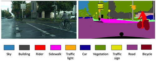
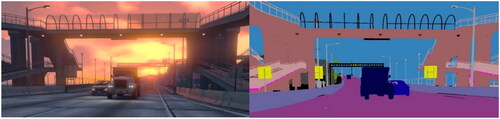
Scene understanding and image interpretation are critical to various machine vision tasks like medical image analysis (Gu et al. 2019; Hesamian et al. 2019), autonomous driving (Chen et al. 2017), and augmented reality (Guan et al. 2020). Semantic segmentation is an essential process in scene understanding as it generates classified raster regions of the input images, which in turn supports the generation of semantic maps. A semantic map layer is produced on top of the geometric map layer by adding semantic objects. Semantic objects, whose identities are distinctly described, define the environment better and help with understanding the map and its information. In the image segmentation process, classes are defined, containing the objects and things in a scenery. For instance, in an urban area image, classes like buildings, cars, humans, streets, and sky could be defined (Figure 1). Then each pixel is annotated to one of the defined classes.

Figure 1. A street view (left) and its semantic segmentation map (right) (Cityscapes dataset).

Deep learning techniques have offered new possibilities for data processing. Supervised learning algorithms learn from training datasets, with the datasets serving as a guide to the learning process. The development of deep learning algorithms can result in the precise prediction of segments in an image. However, to achieve a precise prediction, the supervised learning model should be trained on the same or similar dataset to the one it needs to predict. This not only comes with a great computational price, but it is also very labor-intensive as it requires a large high-quality labeled dataset for training. The process of semantic segmentation with supervised learning has been extraordinarily successful. It begins with data collection, while pre-processing the data, cleaning it, and creating training, validation and test data sets follow.

Another important concern in semantic segmentation with supervised learning is that some categories are substantially more plentiful by default than others, biassing network performance to the more represented ones. For example, in the urban area, the categories of buildings, sky, or roads typically dominate the image. In contrast, categories such as street signs, persons or trees represent a minor number of pixels. Due to the computational expense, as we convolute images during training, these small classes in images shrink even more. Therefore, the prediction accuracy compared to categories that occupy larger portions of the image would likely be smaller. This is an important issue because these smaller underrepresented categories (e.g., humans, cars, traffic signs) are more critical in certain applications such as self-driving cars.

Active learning, (AL), is a form of semi-supervised learning that addresses the need for a vast labeled dataset by actively selecting a subset of the data to be annotated by an "oracle/agent" which could be a human operator or a software. The approaches have been shown to be helpful in lowering training size while maintaining same level of performance. To perform the image classification task, (Joshi et al. 2009) devised a method based on uncertainty sampling. Later, for the same problem, an adaptable active learning strategy was presented (Li and Guo 2013). This strategy combines information density and uncertainty metrics with the selection of critical occurrences to be labeled. The simplest way of addressing the problem of time-consuming labeling would be choosing random regions from images to be labeled. However, this can result in selections that do not contain the most informative regions from the image. Since it is random selection, the performance would also not be stable and reliable.

Generally, for addressing class imbalance problems in the computer vision field, various techniques have been suggested. For example, accuracy is not a good choice of evaluation metrics when we deal with class imbalance. In some cases, over-sampling and under sampling in data preparation is done. We chose a region-based approach in order to address these problems. By using this approach, the “oracle” in charge of labeling the images only labels selected regions from the images. To perform the task of active learning, reinforcement learning approaches are applied. Reinforcement learning is a computational method in which an agent learns to act in an environment based on its interaction with the environment. The agent gets trained through trial-and-error experience to reach a goal while maximizing the reward it obtains from taking an action in the environment. Using a reinforcement learning technique, we chose image regions that contain more underrepresented classes. Essentially, we can use a reinforcement active learning technique to over-sample the underrepresented classes.

In this paper, a modified Deep Q-Learning formulation for active learning is being proposed. An agent learns the method of selecting a collection of small image regions from an unlabeled data pool. These regions provide the segmentation network with the most knowledge by choosing from underrepresented classes. The area of selection is determined by the assumptions and segmentation model uncertainties used during training. The objective is to train a segmentation network by only annotating a small amount of data. Therefore, training dataset is generated in an iterative manner using an active reinforcement learning approach. The iterative process starts with a small pool of training image datasets that train an image segmentation network. Then a small number of unlabeled datasets are chosen to be labeled. The labeled data go through the segmentation network; the trained segmentation model is now evaluated on a subset of data to create state and reward signals for the deep query network (DQN). The state and reward are calculated based on predictions and uncertainties of the segmentation model being trained. Then, based on this feedback, an agent (e.g., a model) in the query network follows a strategy and executes a function to select a small informative region of the image to be labeled from a pool of unlabeled data. The actions taken, based on a specified strategy (policy), are to select regions (states) that are assessed to be more informative by the query network.

The active learning process was carried out by a reinforcement learning agent converging on a policy that selects the action with the highest calculated rewards most of the time (ε-greedy approach). The optimal policy would select the most informative samples from a pool of small regions of the image in order to reduce the annotation labor while maintaining the same level of performance. The contributions of this paper are as follows:

Proposing the use of an active reinforcement learning approach for labeling a small dataset to overcome the need for a significant amount of data to train Deep Neural networks for the task of image semantic segmentation.

Mitigating the bias of underrepresented classes by adopting a Reinforced Active Learning for image segmentation (RALis) strategy with a frequency-weighted average intersection over union (FWA IoU) score to reward the DQN network by putting greater weight on underrepresented classes to improve the network’s performance in these areas even more.

The proposed method’s performance is tested on the well-known Cityscapes urban dataset. The performance of FWA IoU Reinforced Active Learning Image Segmentation (RALis) method is evaluated and analyzed with three baseline segmentation networks trained with image regions selected by the proposed FWA IoU. The backbone network architectures Feature Pyramid Network (FPN) (Lin et al. 2017), DeeplabV3 (Chen et al. 2017), and DeeplabV3+ (Chen et al. 2018) with ResNet-50 (He et al. 2015) are chosen as our segmentation models, considering that they are all sophisticated state-of-the-art semantic segmentation models. Further, the RALis approach performed better compared to baseline region selection by active learning methods such as the Random selection, Entropy-based selection, and Bayesian Active Learning by Disagreement.

The rest of the paper is organized as follows. The related works are discussed in Section 2. The datasets are described in Section 3. Section 4 describes the RALis methodology. The implementation process, experiments and tests are presented in Section 5. Discussions and conclusions are presented in Sections 6 and 7 respectively.

2. Related works

We mainly reviewed reinforcement learning methods that had been used in classification tasks which inspired this work, starting with Casanova et al. (2020), where they developed a data-driven, region-based method to reduce the oracle’s labeling effort in their approach to reinforce active learning for semantic segmentation. This solution tackled the class imbalance problem by using a mean intersection over union (MIoU) performance metric to evaluate the segmentation network’s performance. The Query network is rewarded for selecting useful regions for training the segmentation network, which has the potential to increase the MIoU. Furthermore, with this region-based method, the model can learn to select regions from images that contain the most informative data, which the segmentation model had previously seen less of.

In the work “Playing Atari by deep reinforcement learning,” Mnih et al. (2013) proposed a model for a convolutional neural network trained with a variation of Q-learning; this work demonstrates how a convolutional neural network may overcome hurdles to learning appropriate control policies from raw video input in complicated RL contexts. The network is trained using a variation of the Q-learning technique, with stochastic gradient descent used to update the weights. An experience replay method was employed to address the issues of correlated data and non-stationary distributions. It randomly samples earlier transitions and smooths the training distribution over multiple previous behaviors with raw pixels as input and a value function forecasting future rewards as output.

Liu et al. (2018) leverage expert knowledge from oracle policies to learn a labeling policy. They used an imitation learning method that utilizes an effective algorithmic expert that provides the agent with good actions in the active learning situation. Then a feed-forward network learns the active learning strategy of mapping situations to the most informative data. Later, Bachman et al. (2017) leverage expert knowledge from oracle policies to learn a labeling policy. Meta-learning is used to train a model that learns active learning algorithms (Lake et al. 2019).

Other works rely on policy gradient methods to learn the acquisition function of active learning. Similar to previous work, Pang et al., (2018) also used a meta-learning framework for active learning. Although learning the optimal criterion inside a generic function class is tempting, it does not provide a general solution to AL unless the learned criterion generalizes across varied datasets/learning problems. We can train an excellent query policy for a particular dataset using Deep Reinforcement Learning (DRL), but we need the dataset’s labels to do so; and if we had those labels, we would not need to use AL in the first place. In this work, researchers examine ways to train AL query criteria that generalize across tasks/datasets. This framework defines a Deep Neural Network (DNN) query criterion parameterized by dataset embedding.

Contardo et al., (2017) took a similar meta-learning approach. However, they used a pool-based setting, where the system observes all the examples of the dataset of a problem and has to choose the subset of examples to the label in a single shot. This differs from prior approaches in one-shot learning that considered a stream of instances to classify one after the other. Unlike this work that gathered all labeled data in one step, (Sener and Savarese 2018) propose that a batch of representative samples be chosen to maximize coverage of the unlabeled set. Unfortunately, the bounded core-set loss performs poorly when the number of classes increases.

Woodward and Finn (2017) proposed an active one-shot learning method where unlabeled images are provided one by one, and the decision is to label them or not. They combined meta-learning and reinforcement learning to develop an effective active learning method. In this framework, the deep recurrent model learns to make labeling decisions. They used LSTM (long short-term memory) as their action-value function (Hochreiter and Schmidhuber 1997). Unlike this work, which was stream-based active learning, in some applications, (Konyushkova et al. 2019) used a pool-based active learning method in which unlabeled data is provided beforehand, and the decision is later taken on which samples to choose.

Ebert et al. (2012) used a Markov decision process (MDP) to construct a feedback-driven framework that learns the process during experience without the requirement for prior knowledge (Lim et al. 2016). These strategies just generalize learning the task with less data, ignoring the issues caused by unbalanced classes.

Kampffmeyer et al. (2016) focused on the problem of an imbalanced dataset with remote sensing data. It evaluated the performance of various CNNs on small objects in the image. (Chen et al. 2016) employed a semi-supervised method that uses maximum square loss rather than reducing entropy to avoid relying on a simple strategy of selecting easy-to-transfer data. Konyushkova et al. (2019) developed a data-driven reinforced active learning technique for general use. Because their classification challenge is significantly simpler than the semantic segmentation problem, where DQN training has a higher computational cost. Mackowiak et al. (2018) suggested an approach that concentrated on selecting small sections from images to be labeled by humans to maximize network performance while lowering annotation effort.

Usmani et al. (2021) used reinforced active learning for semantic segmentation for segmentation of road and indoor RGB-D images. Using batch-mode DQN formulation for learning where batches of regions are selected more efficiently for labeling in each iteration, their approach is more computationally efficient and requires fewer labeled data.

Finally, Han et al. (2023) provide an in-depth analysis of various reinforced active learning methodologies for image segmentation where their proposed framework integrates Dueling Deep Q-Networks (DQN), Prioritized Experience Replay, Noisy Networks, and Emphasizing Recent Experience, thus contributing and exploring more sophisticated algorithms across diverse domains.

3. Data

Two open-source urban image datasets were used in our research. The Cityscapes dataset which has a large number of classes alongside many imbalanced classes and the large-scale synthetic GTAv dataset.

3.1. Cityscapes dataset

Cityscapes is a large-scale database focused on the understanding and interpreting urban street scenes. It offers semantic, instance-wise, and dense pixel annotations for 30 classes divided into eight categories (flat surfaces, humans, vehicles, constructions, objects, nature, sky, and void). The dataset contains approximately 5000 finely annotated images. Data was collected in 50 cities over several months, during the day, and in good weather. Because it was initially captured as video, the frames were hand-picked to have the following characteristics: a large number of dynamic objects, a variable scene structure, and a varying background. The image size is 2048 by 1024 in the RGB channels (Cordts et al. 2016). There are two versions of the Cityscapes dataset. One with 35 classes and one with 19 classes. We used the latter one.

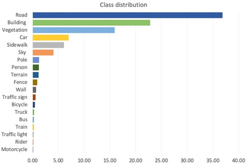
The imbalance is visible in the Cityscapes dataset (Cordts et al. 2016), which is based on street views. In the dataset of 19 classes, the six most underrepresented classes account for less than 2% of the pixels in the training dataset. In contrast, a class-like road takes up more than 36% of the pixels in the training set. This disparity indicates the disparity in the model’s performance (Figure 2)

Figure 2. Imbalanced class distribution in the Cityscapes dataset.

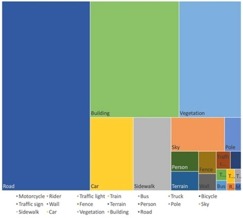
It was used to both train the query network and test the segmentation networks performance trained with regions selected by the query network. The training set contains 2975 images, and the validation set is composed of 500 images (Figure 3). The training data contains images of 18 cities, while validation set contains the images of 3 other cities. As it is a real-world dataset, it is extremely imbalanced. With class Road and Building occupying more than 58% of the total pixels in the whole dataset, 10 most underrepresented classes in total occupy less than 3% of the dataset (Figure 4).

Figure 3. Scene examples from the Cityspaces dataset.

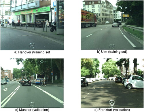
Figure 4. Class distribution in the Cityscapes training set.

3.2. GTAv dataset

The GTAv (Grand theft auto 5) dataset contains 24966 synthetic images with semantic annotation at the pixel level. 12402 images are allocated for the training set, 6347 images for validation, and 6217 images for the test set. The images were created with the open-world computer video game Grand Theft Auto 5 and are all from the perspective of a car driving through the streets of American-style virtual cities. The games’ environment is very appealing for extracting close to real world dataset with least effort as their realism extends beyond the integrity of material appearance and light transport modeling. It can also be found in the game worlds’ content, such as the layout of items and environments, realistic texturing, the movement of vehicles, the existence of little objects that add detail (Richter et al. 2016). GTAv contains images from street scene usually with resolution of 1914 by 1052 pixels (there are few images slightly bigger than mentioned sized in the dataset). We used the GTAv version with 19 semantic classifications which corresponds to Cityscapes dataset with 19 classes. The fact that they are interchangeable with those in the Cityscapes dataset, makes this dataset a perfect one for pre-training the models before training them on the Cityscapes dataset. Additionally, the image size is the same as the cityscape dataset as well (Richter et al. 2016). We split the total 24966 images into 18582 images in training set and 6384 images in validation set (Figure 5). We use the synthetic GTAv dataset to pre-train the segmentation networks before starting the training of the query network.

Figure 5. A scene (left) and its semantic segmentation map (right) (GTAv dataset).

4. Methodology

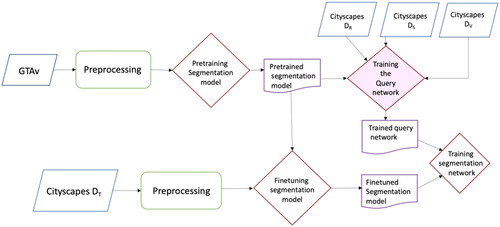
4.1. Reinforced active learning for image segmentation (RALis)

In active reinforcement learning, an agent learns a policy to select small informative regions of the image to be labeled from a pool of unlabeled data. The region selection decision is made based on the performance of the segmentation model being trained. The query network will be represented as a reinforcement learning agent, more specifically as a Deep Q-Network (DQN). A Markov Decision Process (MDP) is used to formulate the Active Learning problem. We express the state space S with the help of a set-aside state set. In this situation, an action is requesting pixel-wise annotation of an unlabeled region from an operator. Because of the large-scale nature of the semantic segmentation job, computing features for each region in the unlabeled set at each step would be prohibitively expensive.

Therefore, the entire unlabeled dataset is approximated by sampling K unlabeled regions. We compute these sub-actions for each region, which has N sampled regions. The agent is rewarded r_t+1 reward which is estimated by the difference in the performance of the segmentation network trained with the newly updated dataset and previous training on the reward dataset. For each state S_t, the agent can take actions A_t to select which samples from the unlabeled dataset to annotate. The MDP is defined by the transition sequence (s_t, a_t, r_t, s_t+1, a_t+1) with s_t ∈ S_t; a_t ∈ A_t; r_t ∈ R_t; s_t+1 ∈ S_t+1; a_t+1 ∈ A_t+1. Each sub-action requests that a specific location be labeled. After training the segmentation network with the given samples, it receives a r_t+1 reward based on the growth in Frequency Weighted Average Intersection-over-Union (FWA IoU) per class (see Section 4.5).

As per the Markov Decision Process, for every state s_t ∈ S, which is a function of segmentation model in timestep t, the agent chooses samples to be annotated from the unlabeled dataset U_t which is action a_t ∈ A. The action a_t= {a_t^k} _k=1,k is also function of segmentation model and it contains K sub-actions, and the sub-actions represent the regions to be labeled. Finally, the query network scores the reward r_t+1 based on the increase on a selected metric FWA IoU after the segmentation network had been trained with chosen samples. To train the query network, a deep Q-network and samples from an experience buffer ε had been employed. We begin by giving the segmentation network a set of initial weights θ₀ with no annotated data.

The process starts with unlabeled U_t and labeled datasets L_t. The labeled data are divided into 4 subsets. We tried to keep the best distribution of classes in each subset. In case of an unlabeled dataset, this could be done through a visual assessment of the images. Also, the number of images in each subset is kept to a minimum efficient number. We started the experiments with least reasonable amount of data, where:

• Training dataset D_T, on which active learning process had learnt an optimal acquisition function which would achieve best performance on data budget B of labeled regions.

• Reward dataset D_R, to provide a reward signal to evaluate the performance of the segmentation network on chosen regions.

• State dataset D_S, to generate a representation of the state.

• Validation set D_V, on which the query network is evaluated.

Prior to training the query network, the segmentation network had been pretrained on a synthetic dataset, in this case the GTAv (Richter et al. 2016), and fine-tuned on the D_T. The steps of the reinforced active learning method for each iteration t shown in Figure 6 are:

Figure 6. The architecture of end-to-end Active Reinforcement Learning model.

1. The state of the Q network is computed as a function of the segmentation network on the state set D_S.

2. The regions that were uniformly selected from the unlabeled set are combined to form an action pool. A sub-action representation has been calculated for each action a^K_t.

3. Following that, the query network employs an ε-greedy technique to choose sub-actions from the action pool. The ε-greedy policy is an action selection policy in which the agent exploits prior information while simultaneously exploring other alternatives. Most of the time, this technique selects the action with the most considerable estimated reward.

4. The query network’s chosen regions are annotated by the human operator acting as an oracle, and these annotated regions are included in the training set.

5. The segmentation network is trained on the training set and then evaluated on the reward set D_R.

6. The improvement in the segmentation network’s performance on the reward set D_R in one iteration compared to the previous one provides the query network agent with a reward reflecting how well it did in selecting the most informative regions of the images. In case there was no improvement in performance of the network, this policy would not be selected as optimal policy.

This cycle is repeated until a budget B of labeled regions is reached, which is the predefined number of regions the query network could ask to be labeled.

4.2. Deep query network (DQN)

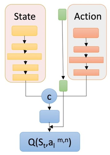
The Deep Query Network (DQN) solves the problem where the Q-table can only store a limited number of states, where in actual applications the number of states could be extremely large. DQN combines the traditional Q-learning method with the deep CNN. Query network converges to a policy that maps a state to an action that would optimize the future reward. A labeled set D_T is used to train the DQN parametrized by ϕ and a held-out split D_R to compute the rewards. The query agent selects K regions before moving on to the next state. Applying a batch-mode DQN formulation for learning, where batches of regions are selected for labeling in each iteration, supports computational efficiency and requires less labeled data. The assumption is that each region is chosen individually, as in the case of K annotators labeling one region concurrently. In this situation, the action is formed into K separate sub-actions {a^k_t}_k=1,K each with a limited action space, avoiding the action space’s combinatorial explosion (Equ. 1(1) $$a_t^k=\begin{array}{c}\mathit{\text{argmax}}\\ a_t^{k,n}\in {\rho }_t^k\end{array}Q\left(s_t,a_t^{k,n};\varnothing \right)$$(1) ). We restrict each sub-action a^k_t to selecting a region x_k in P_t^k for each k = {1,…, K} action taken in timestep t to simplify computations and avoid selecting repeated regions in the same time-step (Casanova et al. 2020). (1) $$a_t^k=\begin{array}{c}\mathit{\text{argmax}}\\ a_t^{k,n}\in {\rho }_t^k\end{array}Q\left(s_t,a_t^{k,n};\varnothing \right)$$(1)

The network is trained by optimizing a loss based on the temporal difference (TD) error (Sutton and Barto 2018). The loss is defined as the expectation over deconstructed transitions generated from standard transitions (Casanova et al. 2020). E is the experience replay buffer, and y_t^k is the TD target for each sub-action (Equ. 2(2) $${\mathbb{E}}_{\mathcal{T}}\sim \left[{\left(y_t^k-Q\left(s_t,a_t^k;\varnothing \right)\right)}^2\right]$$(2) ). (2) $${\mathbb{E}}_{\mathcal{T}}\sim \left[{\left(y_t^k-Q\left(s_t,a_t^k;\varnothing \right)\right)}^2\right]$$(2)

The target network with weights and the double DQN formulation was used for a more stable training process (van Hasselt et al. 2015). The selection and evaluation of actions are decoupled; the action is chosen with the target network and evaluated with the query network. The TD target for each sub-action is computed as explained in Equation 3(3) $$y_t^k=r_{t+1}+\gamma Q\left(s_{t+1},\begin{array}{c}\mathit{\text{argmax}}\\ a_{t+1}^{k,n}\in {\rho }_{t+1}^k\end{array}Q\left(s_{t+1},a_{t+1}^{k,n};{\varnothing }^{\prime }\right);\varnothing \right)$$(3) where γ represents the discount factor (Casanova et al. 2020). (3) $$y_t^k=r_{t+1}+\gamma Q\left(s_{t+1},\begin{array}{c}\mathit{\text{argmax}}\\ a_{t+1}^{k,n}\in {\rho }_{t+1}^k\end{array}Q\left(s_{t+1},a_{t+1}^{k,n};{\varnothing }^{\prime }\right);\varnothing \right)$$(3)

The query network is comprised of two paths: one for computing state representation and another for computing action representation, which are then fused at the end (Figure 7). Each layer includes Batch Normalization, ReLU activation, and a fully-connected layer. The state path is composed of four layers and action is built up from three layers. A final layer merges them together to produce the global features, which are gated by a sigmoid and controlled by the Kullback-Leibler (KL) probability divergence score in the action representation. At each step of the active learning loop, the weights are modified by sampling batches of 16 experience tuples from an experience replay buffer. For probabilities Q and P, the KL divergence can be calculated as the negative sum of each event’s probability in P multiplied by the log of the event’s probability in Q over the probability of the event in P (Equ. 4; Ganegedara 2018). (4) $$\mathit{\text{KL}}\left(P\parallel Q\right)=-\sum _{xϵX}P\left(x\right)\mathrm{\text{log}}\hspace{0.17em}\left(\frac{P\left(x\right)}{Q\left(x\right)}\right)$$(4)

Figure 7. Query network architecture.

4.3. State representation

The MDP state is defined as the state of the segmentation network. As we cannot directly embed the segmentation network into state representation, as per a suggestion in Konyushkova et al., (2017), the state is represented with the D_S dataset. The D_S is designed to represent all classes the best it can. When a new dataset is being labeled, this would be done by a visual estimation of classes in selected images. For best results, the class distribution in D_S should represent that of the training dataset. To generate the global state representation St, the prediction of the segmentation network from D_S is used. To prevent high memory consumption due to pixel-wise predictions, we require a compact representation. In D_S, samples are divided into patches, and compact feature vectors are produced for each of them. In D_S, each area x_i is represented as a concatenation of two features, one based on entropy and one on class predictions. The ultimate state S_t is the concatenation of all regions features.

The first set of features is a normalized count of how many pixels are predicted to belong to each category. This feature encodes the segmentation forecast of a specific patch while ignoring spatial information, which is less essential for small patches. Furthermore, we calculate the predictor’s uncertainty using entropy over the likelihood of predicted classes. Entropy measures the amount of information in a random variable, more especially its probability distribution. In relation to a reference measure ρ, the Shannon entropy of a random variable X with distribution μ is (Equ. 5; Shalizi): (5) $$H_{\rho }\left[X\right]\equiv -E_{\mu }\left[\mathrm{\text{log}}\hspace{0.17em}\frac{d\mu }{d\rho }\right]$$(5)

To generate a spatial entropy map, we compute the entropy of each pixel location in each region. We apply min, average, and max-pooling to the entropy map to create down sampled feature maps in order to compress this representation. The second set of features is consequently created by flattening and concatenating these entropy features.

4.4. Action representation

Executing an action is requesting the pixel-by-pixel annotation of an unlabeled region. Due to the large-scale nature of semantic segmentation, computing features for each location in the unlabeled set at each step would be prohibitively expensive. As a result, at each step t, we approximate the entire unlabeled set by sampling K pools of unlabeled regions P_t^k, each of which contains N (uniformly) sampled regions. We compute the sub-action representation a_t^k,n for each region. Each sub-action a_t^k,n is a concatenation of four distinct features:

1. The entropy feature,

2. Class distribution features (as in the state representation),

3. A measure of similarity between the region x_k and the labeled set,

4. Another measure of similarity between the region and the unlabeled set.

The idea is that the query network can learn to produce a more class-balanced labeled set while continuing sampling from the unlabeled set. This could help to minimize the segmentation dataset’s hard imbalance and enhance overall performance.

Kullback-Leibler (KL) Divergence is merely a simple change to the entropy formula. The probability distribution is merged with the approximation distribution. We compute the KL divergence between the class distributions of the prediction map of region x and the class distributions of each labeled and unlabeled region for each candidate region, x, in a pool P_t^k (using the ground-truth annotations and network predictions, respectively).

For the labeled set, we compute a KL divergence score between the class distributions of the labeled areas and the one of region x. Taking the maximum or adding all of these KL divergences could be used to summarize them. To extract informative features, a normalized histogram of KL divergence was calculated. The same process had been followed for the unlabeled dataset to obtain another KL divergences distribution. And finally, they are concatenated to action representation.

4.5. Evaluation metric and rewards calculation

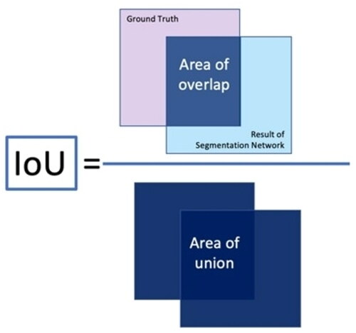
The Intersection-Over-Union (IoU), often known as the Jaccard Index, is a popular metric to evaluate the performance of semantic segmentation task (Equ. 6; Figure 8). The Mean IoU of the image is calculated for binary (two classes) or multi-class segmentation by averaging the IoU of each class. IoU value would naturally range from 0 to 1, with 1 denoting perfect segmentation. (6) $$\mathit{\text{IoU}}=\frac{\mathit{\text{TP}}}{\mathit{\text{TP}}+\mathit{\text{FP}}+\mathit{\text{FN}}}$$(6)

Figure 8. Intersection over union.

Instead of penalizing the query network using the Mean IoU measure, in this work we employed a Weighted Average of IoU across classes based on the frequency of the classes to focus even more attention on the underrepresented classes. Instead of taking the mean of IoU, we calculated the W_c as the weight of each class that is inversely proportional to its fc frequency which is number of pixels of each class (Equ. 7), where ε is just a very small value we add to frequency to avoid the complication in case of classes with zero frequency (Mohapatra et al. 2021). (7) $$W_c=\frac{1}{\mathrm{\text{log}}(f_c+\epsilon )}$$(7)

Frequency Weighted Average IoU, (FWA IoU), is an extension of the IoU statistic that is used to prevent class imbalance. If one class dominates the majority of the images in a dataset, such as the “Building” class, this class must be brought down in comparison to other classes. The weighted average s is calculated based on the frequency of the class region in the dataset where the high-frequency classes get lower weight and low-frequency classes get larger weight.

5. Implementation

In our experiments, we have the data initially pre-processed (step 1). Then, we trained all the segmentation networks on a large-scale GTAv synthetic dataset (step 2). Afterwards, the networks are fine-tuned on the Cityscapes training subset containing 150 images (step 3). Following this, the Query network was trained to learn the best policy that would select the most informative image regions (step 4). We evaluated the performance of the query network using different selected data budgets of labeled regions with three baseline image segmentation networks (Feature Pyramid Network, DeepLabV3 and DeepLabV3+) and three active learning methods of Random Selection, Entropy-based Selection, and Deep Bayesian Active Learning (BALD) (step 5). Finally, the performance of the RALis approach compared to the supervised method in all segmentation networks was assessed (step 6). The implementation process is illustrated in Figure 9.

Figure 9. Implementation flowchart.

5.1. Step 1: Dataset division and preprocessing

The training data had been partitioned to four sub-sets in order to train the query network and evaluate the performance of the trained segmentation network on regions chosen from the query network. Table 1 lists the number of images on each sub-set. We try to use the least amount of data possible. The query network needs 360 images in total, which is 12% of all training data and 8% of all the dataset.

Table 1. The Cityscapes dataset partition.

DS	DT	DR	DV
10	150	200	2615

For these experiments, as we have very large images in the dataset, we randomly crop smaller regions from images to overcome memory problems with larger batch sizes; in various steps, we use different region sizes (the respective region size will be mentioned). We performed a random horizontal flip in all steps of training, and additionally we applied standard normalization to all images.

5.2. Step 2: Pre-training the segmentation networks with GTAv synthetic dataset

For pre-training the segmentation networks on the GTAv dataset, we used images cropped to 1904 by 1024 pixels to have uniformly sized images. We used a pre-trained ResNet-50 as backbone from Pytorch library which had been trained on the ImageNet dataset. We used a learning rate of 10 × e-3 with gamma rate of 0.995 and training batch size of 4. Additionally, we used an Adam optimizer and weighted cross entropy loss function. We also tried an SGD optimizer (Stochastic Gradient Descent), however we obtained better results with the Adam optimizer.

We used a patience of 70 epochs for this set of training, which means if validation Mean IoU does not increase in 70 epochs, we would stop the training. The benefit of training with the GTAv synthetic dataset is that the data is very similar, and it helps the model to generalize better. In all networks, we froze the pre-trained backbone at the beginning of our experiment and train it with learning rate of 10 × e-3. Later we unfroze the backbone and trained it with smaller learning rate of 10 × e-4. We then proceeded to unfreeze it and trained it with a learning rate of 10 × e-4.

We used three state-of-the-art segmentation network architectures: Feature Pyramid Network (FPN), DeepLabV3, and DeepLabV3+. The weighted cross entropy was used as loss function. Table 2 lists the settings of our experiment.

Table 2. Pretraining details.

	Backbone	Input Size	Learning Rate	Loss	Batch size	Optimizer	Validation Mean IoU
FPN	ResNet-50	1904 $\times$1024	10 $\times$ e-3,10 $\times$ e-4	Weighted cross entropy	4	Adam	73%
DeepLabV3	ResNet-50	1904 $\times$ 1024	10 $\times$ e-3,10 $\times$ e-4	Weighted cross entropy	4	Adam	73%
DeepLabV3+	ResNet-50	1904 $\times$ 1024	10 $\times$ e-3,10 $\times$ e-4	Weighted cross entropy	4	Adam	74%

The DeepLabV3+ segmentation network achieved slightly better results compared to other two networks. It is worth mentioning that by changing the setting of the network and conducting more experiments, we can achieve a better validation of the Mean IoU on the networks. But since the sole purpose is to pre-train the network so that the segmentation network initiates at a better point, we did not focus on obtaining the best results from this experiment. The results are shown in Figure 10.

Figure 10. Pre-training FPN, DeepLabV3, and DeepLabV3+ segmentation networks on GTAv synthetic dataset.

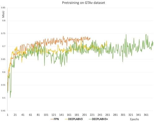
This step is very time consuming. A GeForce RTX 3090ti GPU was used, which has a RAM of 24 GB and CUDA Cores: 10,753. Base Clock Speed: 1670 MHz. Boost Clock Speed: 1890 MHz (as tested, stock is 1860 MHz). Each experiment took around 250 hours.

5.3. Step 3: Fine-tuning the segmentation networks on a training subset of cityscapes

After pre-training the segmentation networks on GTAv dataset, we fine-tuned the segmentation networks with 150 images from the training Cityscapes dataset D_T. As inputs for the network, we used random images cropped to 512 by 1024 pixels. For fine-tuning, we first froze the backbone and used a learning rate of 10 x e-5 with the gamma rate of 0.995 and training batch size of 16. Later we unfroze the backbone and used a backbone of 10 x e-6 to train the network some more so all layers would have been fine-tuned, using a very small learning rate to prevent divergence. We arrived at this method of freezing and unfreezing the backbone, following experimentation with completely freezing the network or freezing part of backbone instead of all. The optimizer and loss functions are the same as ones we used to pre-train the GTAv dataset. Again, we used a batch of 100 epochs for early stopping of the training process. The details on fine-tuning are given in Table 3. Since the model had been trained on a very compatible training set of GTAv, it performed well at this stage and achieved over 50% Mean IoU on each of these segmentation networks. Figure 11 shows the training results of the Mean IoU.

Figure 11. Fine-tuning on D_t subset.

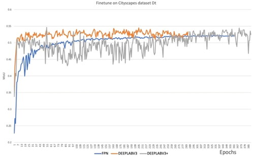
Table 3. Fine-tuning details.

	Backbone	Input Size	Learning Rate	Loss	Batch size	Optimizer	Validation Mean IoU
FPN	ResNet-50	512 $\times$1024	10 $\times$ e-5, 10 $\times$ e-6	Weighted cross entropy	16	Adam	52.2%
DeepLabV3	ResNet-50	512 $\times$ 1024	10 $\times$ e-5, 10 $\times$ e-6	Weighted cross entropy	16	Adam	54.4%
DeepLabV3+	ResNet-50	512 $\times$ 1024	10 $\times$ e-5, 10 $\times$ e-6	Weighted cross entropy	16	Adam	64.6%

5.4. Step 4: Query network - training of the DQN network

To build the action pool for the query network, the query network is trained on the Cityscapes training dataset D_T. At each step, the DQN state is computed, and 256 regions of 128 by 128 pixels are selected. The acquisition functions performance is tested by having it select the regions from D_V until the budget of 3840 regions is met. We chose this number, which is 1% of the dataset, because it was sufficient. The segmentation network is then trained with the labeled data chosen (256 × 512 crops) until the early stopping condition is met on D_R. Then the reward is calculated.

As mentioned before, this method is data driven and by default, due to using the increase on Mean IoU to compute reward, we increased the performance of the network on underrepresented classes. To further address the class imbalance issue, we used the Frequency Weighted Average IoU for calculating the reward of segmentation network.

At the end, the acquisition function with the best reward result is chosen. For training the query network, we used a learning rate of 10 × e-4 for both DQN and segmentation networks. The computation of the state takes the longest time during this stage. The DQN query network had been trained for 50 epochs. Full resolution images were also used, and each epoch took approximately one hour.

This is one of the downsides of the RALis method (Reinforcement Active Learning for image segmentation), where pre-training, fine tuning and training the Query network might take up to two weeks (based on the available computer resources). However, if our goal is to take advantage of an unlabeled dataset, this still saves time and resources since it would optimize the human assistance required to label the dataset. In each episode, the Query network chooses 256 more regions and when it reaches the budget of 3840 regions, it trains the model for 16 epochs with the chosen data. Then the query network is evaluated based on its performance on the reward set, and the state is again computed. Finally, the optimal policy is saved to be tested on the segmentation network.

After acquiring the acquisition function by training the query network, we test the policy by training the segmentation network with six small budgets of regions chosen by the query network. The budget varies from 0.5% of the training dataset to 8%, which equals 1920, 3840, 7680, 11520, 19200, and 30720 regions (Table 4). We chose regions with the size of 256 by 512 pixels. We used the learning rate of 10 × e-6, training batch size of 16, and gamma rate of 0.995 alongside Adam optimizer. Patience of 70 epochs was used in this step as well.

Table 4. Percentage of region numbers from all of the dataset.

Regions number	1920	3840	7680	11520	19200	30720
Percentage	0.5%	1%	2%	3%	5%	8%

5.5 Step 5: Segmentation networks and active learning baseline approaches on the budgeted regions

We evaluate the query networks policy with various data budgets with the three supervised learning segmentation networks. The results were also compared with three active learning policies, Random selection, selection based on Entropy, and Bayesian Active Learning by Disagreement (BALD) method (Gal et al. 2017) since they were the primary and best available methods, where,

1. Random is the uniform random sampling of regions from action pool,

2. The Entropy method is an uncertainty sampling method which applies the active learning policy of choosing maximum pixel-wise Shannon entropy,

3. Bayesian Active Learning by Disagreement (BALD) method selects the regions based on maximum cumulative pixel-wise BALD metric (Gal et al. 2017).

Note that all methods used a model that had been pre-trained on the GTAv dataset and then fine-tuned on D_V. Pool sizes of 500, 200, 200 and 100 were used respectively for random, entropy, Bayesian and the proposed method from this work. Pool sizes were determined in accordance with the best validation Mean IoU.

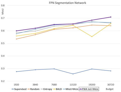
5.6. Step 6a: Using RALis with the FPN segmentation network

We test the query networks policy with various data budgets on several segmentation networks. The results were compared with other active learning policies like Random selection, selection based on Entropy and BALD method. For the FPN model we used the Mean IoU and Frequency Weighted Average IoU to compute the reward of the query network (Table 5). In Figure 15, the graph demonstrates that rewarding the query network based on the Frequency Weighted Average IoU achieves the best result, only slightly better than using Mean IoU. From this point on, we only experimented with rewarding query network with Frequency Weighted Average IoU.

Table 5. Comparison of performance of the FPN network across various methods with different budgets (MIoU).

Budget	Supervised	Random	Entropy	BALD	MioU RALis	FWA IoU RALis
1920	0.28	0.53	0.59	0.56	0.58	0.60
3840	0.29	0.57	0.60	0.58	0.61	0.62
7680	0.30	0.61	0.64	0.62	0.65	0.65
11520	0.26	0.62	0.65	0.64	0.66	0.65
19200	0.30	0.65	0.67	0.55	0.67	0.68
30720	0.28	0.64	0.66	0.66	0.67	0.71

Additionally, a budget with 1920 samples of supervised network is equal to 15 images in Cityscapes dataset. The model is trained with weights saved from fine-tuning on D_t dataset and the results are worse and not even comparable with other active learning methods. As Figure 12 indicates, the results of the supervised method with an equal number of images to the data budget are comparably very low. This indicates that the supervised method does not perform well with a small amount of data.

Figure 12. Performance of our method with the FPN segmentation network compared to baselines.

Further, to understand the effect of using the FWA IoU method in comparison to the Mean IoU, Figure 13 shows the Mean IoU on 6 underrepresented classes. The Frequency Weighted Average IoU outperforms the RALis Mean IoU method in six of the most underrepresented classes.

Figure 13. The performance of the RALis method rewarded by MIoU and FWA IoU.

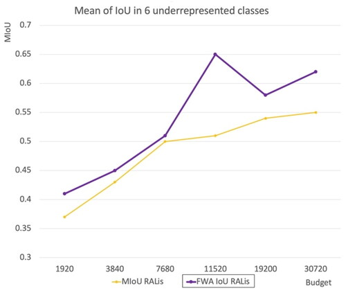
Table 6 shows the performance of the RALis FWA IoU method on six underrepresented classes. From the percentage of each class, it can be seen that all the six classes in total occupy less than 1.5% of the Cityscapes training set. However, using 8% budget regions, they achieved between 42 to 66% MIoU (Figure 13).

Table 6. Performance of our method on six underrepresented classes (MIoU).

Budget	Bicycle	Motorcycle	Train	Bus	Truck	Rider	Total
1920	0.39	0.34	0.28	0.50	0.38	0.61	0.42
3840	0.40	0.37	0.32	0.54	0.48	0.64	0.46
7680	0.42	0.46	0.41	0.63	0.52	0.66	0.52
11520	0.44	0.54	0.44	0.46	0.65	0.48	0.66
19200	0.54	0.51	0.49	0.72	0.59	0.69	0.59
30720	0.54	0.63	0.61	0.72	0.52	0.72	0.62
Pixel %	0.41	0.10	0.23	0.24	0.27	0.14	1.39

5.7 Step 6b: Using RALis with the DeepLabV3 segmentation network

Using the RALis method with DeepLabV3 achieved the best result in comparison to the baselines from all other budgets. However, the results are not as good as those achieved by the FPN network. Figure 14 illustrates the results of this experiment.

Figure 14. Our RALis method with DeepLabV3 segmentation network in comparison to other baselines.

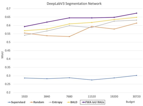
According to Table 7, a segmentation network had the best performance across all budgets once it had been trained by regions selected by a query network that had been rewarded with FWA IoU.

Table 7. The comparison of performance of the DeepLabV3 network across various methods with different budgets (MIoU).

Budget	Supervised	Random	Entropy	BALD	FWA IoU RALis
1920	0.29	0.55	0.54	0.30	0.59
3840	0.28	0.54	0.57	0.58	0.62
7680	0.29	0.53	0.60	0.61	0.65
11520	0.28	0.59	0.59	0.62	0.65
19200	0.29	0.58	0.63	0.63	0.65
30720	0.30	0.61	0.63	0.65	0.67

5.8 Step 6c: Using RALis with the DeepLabV3+ segmentation network

DeepLabV3+ achieved the best results in comparison to other baselines in most budgets, however, in a budget of 3840 regions, Random selection obtained the best result and even surpassed the performance of RALis with 7680 budgets. But, for the last three budgets, RALis performed better than the other methods. Also, a deeper look at the graphs suggests that the performance of the RALis method decreased on 3840 dataset budget, indicating that in this budget, the RALis methods did not perform as well (Figure 15).

Figure 15. RALis method with a DeepLabV3+ segmentation network in comparison to other baselines.

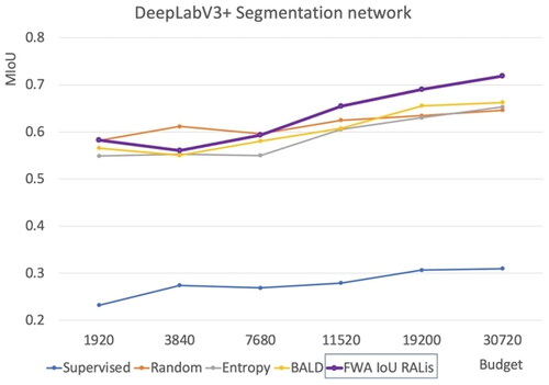
As displayed in Table 8, the DeepLabV3+ network performs the best in most budgets with regions selected by a query network that had been rewarded with FWA IoU, in comparison to Random selection of regions, Selection of regions based on Entropy, and the BALD method, respectively.

Table 8. The comparison of performance of the DeepLabV3 network across various methods with different budgets (MIoU).

Budget	Supervised	Random	Entropy	BALD	FWA IoU RALis
1920	0.23	0.58	0.55	0.56	0.58
3840	0.27	0.61	0.55	0.55	0.56
7680	0.27	0.60	0.55	0.58	0.59
11520	0.28	0.62	0.61	0.61	0.65
19200	0.31	0.63	0.63	0.66	0.69
30720	0.31	0.65	0.65	0.66	0.72

5.9 Step 6d: Comparison of RALis with fully supervised methods

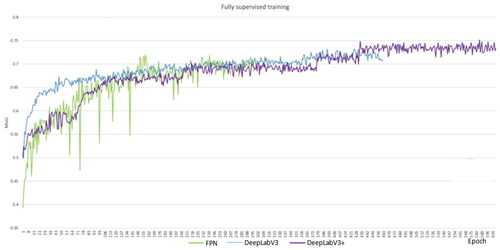
In order to have good baseline data, we also did a fully supervised training for the segmentation models on the Cityscapes dataset (Figure 16). We used the fine-tuned method instead of initiating the models’ weights from scratch in order to have a fair comparison. For this experiment, we used full-size Cityscapes images with training batch size of 4 and a learning rate of 10 × e-6.

Figure 16. The segmentation models are trained on all of the Cityscapes dataset, containing 2975 images. The results are compared to IoU for validation.

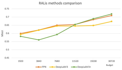
In Figure 17, we compare the performance of the segmentation networks trained with regions chosen by reinforced active learning methods. The DeepLabV3+ performs the best on the last two budgets; however, with budgets 3840, and 7680, it falls significantly behind the other two networks. This suggests that DeepLabV3+ might be the superior method with more than 5% of the dataset budget, however with smaller budgets it does not outperform others.

Figure 17. A comparison of the performance of the RALis method rewarded with weighted IoU.

The FPN network with reinforced active learning method achieved a 98.7% success rate on 8% of the total data budget in comparison to the fully supervised process. In comparison, DeepLabV3 achieved 91.9% and DeepLabV3+ achieved 95.6% (Table 9).

Table 9. The performance of supervised and FWA RALis methods across three networks (MIoU).

	Supervised (100% datd)	FWA RALis (8% data)
FPN	71.8%	70.9%
DeepLabV3	73.2%	67.3%
DeepLabV3+	75.1%	71.8%

As shown in Table 10, the FWA IoU RALis method achieves better results than all other region selection methods across all three segmentation networks, in comparison with our three baselines.

Table 10. The performance of baselines and RALis method across three networks with 8% budget of all data (MIoU).

	Random	Entropy	BALD	FWA IoU RALis
FPN	64%	66%	66%	71%
DeepLabV3	61%	63%	65%	67%
DeepLabV3+	65%	65%	66%	72%

6. Discussion

We used the reinforcement learning agent as an acquisition function for the active learning method. The query network selects a batch of the most informative regions in the images and chooses them to be labeled by human operator. Afterward, the selected regions are added to the labeled dataset and the segmentation network is trained with these data. Subsequently, the performance of the segmentation network is evaluated on the reward set. Then query network is rewarded based on the validation of the Frequency Weighted Average IoU across all classes. The same cycle continues until an optimal policy is reached by the query network to choose the most informative regions within the specific budget.

For testing the performance of the query network, we tested it on three segmentation networks. The query network chooses the number of regions based on the budget. Then the segmentation network, which had been previously trained on the synthetic GTAv dataset and then fine-tuned on the training set with 150 images from the Cityscapes dataset, is trained with selected regions. The performance is tested by the MIoU evaluation metric with various baselines, including the fully supervised method. We used three different architectures as the segmentation network, and comprehensive experiments are conducted. Additionally, the performance of underrepresented classes increases noticeably. However, it is important to note that in order to make this method work, we need a synthetic dataset which would have similar content and match the classes of our data. We have successfully trained a query network to select informative regions of each image to be labeled. To train the query network, 340 full-size images were used, which is equal to 8% of dataset. We examined the query network performance with various budgets of labeled regions. The budgets varied from 0.5% of the dataset, which is 1920 image regions of 128 by 128 pixels, to 8%, which would be 30720 regions of same size. We trained three state-of-the-art segmentation networks using the reinforced active learning approach. All three segmentation networks achieved better results using the 8% budget with the FWA-IoU RALis method in comparison to the selected baseline methods of Random selection, Entropy-based active learning selection, and the BALD method. The equivalent MIoU training performances compared to image segmentation using the fully supervised approach were 98.7% for the FPN network, 91.9% for the DeepLabV3, and 95.6% for the DeepLabV3+.

7. Conclusions

In this study, we aimed to improve the deep learning method for image segmentation by suggesting an end-to-end active reinforcement learning method. The active reinforcement learning method could be used while labeling the collected data, in order to only label the image regions with most important information. Active learning helps to intelligently select and label a portion of the data and the learning algorithm performs well with smaller amounts of data. It allows the query agent to request data based on their characteristics and class imbalances across the datasets. Since the Frequency Weighted Average IoU is optimized per class using reinforcement learning, more under-represented labels are selected.

Reinforcement learning does not depend on the training data as in the case of the supervised learning models. The reinforcement model decides what to do based on the state-action reward model that helps to determine the correctness of the action. Considering the small amount of training data required and the reward condition, the model is expected to be less sensitive to human data annotation errors.

The experiments show that we obtained excellent results by using a synthetic dataset to train the network, while only labeling 8% of the dataset to train the query network and another 8% to train the segmentation network. The experiments show that the Reinforced Active Learning method for image segmentation performs well with various segmentation networks. The FPN achieved almost 98% of the effects the network could achieve with the Cityscapes datasets. The other two segmentation networks also achieved excellent results. Also, it comparably achieves better results than all other tested active learning baseline methods with the same data budgets. This method can save the operators time on labeling the data while achieving the same level of performance.

There are some limitations to this work. As mentioned, to pre-train the segmentation networks, a compatible synthetic dataset is needed. The quality of the training data is directly reflected in the predictions of the segmentation networks. Another limitation is the length of training time related to the query network, and the pre-training of the segmentation network.

Regarding the semantic segmentation task, future work could employ more imbalanced datasets with different characteristics. For instance, datasets collected with other mobile sensors such as UAVs and indoor scene data collected by mobile robot sensors.

Further it is important to study the effect of the quality and quantity of the reward and state set on training and performance of the query network. Additional studies could be conducted on the budget of the labeled data for training the query network.

Additional information

Funding

This work has been financially supported by the Natural Sciences and Engineering Research Council of Canada (NSERC Discovery Grant) and York University.

References

- Bachman, P., Sordoni, A., and Trischler, A. 2017. “Learning Algorithms for Active Learning.” doi:10.48550/arXiv.1708.00088.
- Casanova, A., Pinheiro, P. O., Rostamzadeh, N., and Pal, C. J. 2020. “Reinforcement Active Learning for Semantic Segmentation.” doi:10.48550/arXiv.2002.06583.
- Chen, B., Gong, C., and Yang, J. 2017. “Importance-Aware Semantic Segmentation for Autonomous Driving System.” Proceedings of the Twenty-Sixth International Joint Conference on Artificial Intelligence. Melbourne, Australia, pp. 1504–1510. doi:10.24963/ijcai.2017/208.
- Chen, L.-C., Papandreou, G., Kokkinos, I., Murphy, K., and Yuille, A.L. 2016. “Semantic Image Segmentation with Deep Convolutional Nets and Fully Connected CRFs.” IEEE Transactions on Pattern Analysis and Machine Intelligence, Vol. 40(No. 4): pp. 834–848. doi:10.1109/TPAMI.2017.2699184.
- Chen, L.-C., Papandreou, G., Schroff, F., and Adam, H. 2017. “Rethinking Atrous Convolution for Semantic Image Segmentation.” ArXiv170605587 Cs.
- Chen, L.-C., Zhu, Y., Papandreou, G., Schroff, F., and Adam, H. 2018. “Encoder-Decoder with Atrous Separable Convolution for Semantic Image Segmentation.” ArXiv180202611 Cs.
- Contardo, G., Denoyer, L., and Artières, T. 2017. “A meta-learning approach to one-step active learning.” arXiv preprint arXiv:1706.08334.
- Cordts, M., Omran, M., Ramos, S., Rehfeld, T., Enzweiler, M., Benenson, R., Franke, U., Roth, S., and Schiele, B. 2016. “The Cityscapes Dataset for Semantic Urban Scene Understanding.” ArXiv160401685 Cs.
- Ebert, S., Fritz, M., and Schiele, B. 2012. “RALF: A Reinforced Active Learning Formulation for Object Class Recognition.” Presented at the 2012 IEEE Conference on Computer Vision and Pattern Recognition (CVPR), IEEE, Providence, RI, pp. 3626–3633. doi:10.1109/CVPR.2012.6248108.
- Gal, Y., Islam, R., and Ghahramani, Z. 2017. “Deep Bayesian Active Learning with Image Data.” ArXiv170302910 Cs Stat.
- Ganegedara, T. 2018. “Intuitive Guide to Understanding KL Divergence.” https://towardsdatascience.com/light-on-math-machine-learning-intuitive-guide-to-understanding-kl-divergence-2b382ca2b2a8
- Gu, Z., Cheng, J., Fu, H., Zhou, K., Hao, H., Zhao, Y., Zhang, T., Gao, S., and Liu, J. 2019. “CE-Net: Context Encoder Network for 2D Medical Image Segmentation.” IEEE Transactions on Medical Imaging, Vol. 38(No. 10): pp. 2281–2292. doi:10.1109/TMI.2019.2903562.
- Guan, P., Cao, Z., Chen, E., Liang, S., Tan, M., and Yu, J. 2020. “A real-time semantic visual SLAM approach with points and objects.” International Journal of Advanced Robotic Systems, Vol. 17(No. 1): pp. 172988142090544. doi:10.1177/1729881420905443.
- Han, D., Huong, P., and Cheng, S. 2023. “Enhancing Semantic Segmentation through Reinforced Active Learning: Combating Dataset Imbalances and Bolstering Annotation Efficiency.” Journal of Electronic & Information Systems, Vol. 5(No. 2): pp. 45–60. doi:10.30564/jeis.v5i2.6063.
- He, K., Zhang, X., Ren, S., and Sun, J. 2015. “Deep Residual Learning for Image Recognition.” ArXiv151203385 Cs.
- Hesamian, M.H., Jia, W., He, X., and Kennedy, P. 2019. “Deep Learning Techniques for Medical Image Segmentation: Achievements and Challenges.” Journal of Digital Imaging, Vol. 32(No. 4): pp. 582–596. doi:10.1007/s10278-019-00227-x.
- Hochreiter, S., and Schmidhuber, J. 1997. “Long Short-term Memory.” Neural Computation, Vol. 9(No. 8): pp. 1735–1780. doi:10.1162/neco.1997.9.8.1735.
- Joshi, A. J., Porikli, F., and Papanikolopoulos, N. 2009. “Multi-Class Active Learning for Image Classification.” Presented at the 2009 IEEE Computer Society Conference on Computer Vision and Pattern Recognition Workshops (CVPR Workshops), IEEE, Miami, FL, pp. 2372–2379. doi:10.1109/CVPR.2009.5206627.
- Kampffmeyer, M., Salberg, A.-B., and Jenssen, R. 2016. “Semantic Segmentation of Small Objects and Modeling of Uncertainty in Urban Remote Sensing Images Using Deep Convolutional Neural Networks.” Presented at the 2016 IEEE Conference on Computer Vision and Pattern Recognition Workshops (CVPRW), IEEE, Las Vegas, NV, USA, pp. 680–688. doi:10.1109/CVPRW.2016.90.
- Konyushkova, K., Sznitman, R., and Fua, P. 2019. “Discovering General-Purpose Active Learning Strategies.” ArXiv181004114 Cs Stat.
- Konyushkova, K., Sznitman, R., and Fua, P. 2017. “Learning Active Learning from Data.” Advances in Neural Information Processing Systems, Vol. 30, pp. 4225–4235.
- Lake, B.M., Salakhutdinov, R., and Tenenbaum, J.B. 2019. “The Omniglot challenge: a 3- year progress report.” Current Opinion in Behavioral Sciences, Vol. 29 pp. 97–104. doi:10.1016/j.cobeha.2019.04.007.
- Li, X., and Guo, Y. 2013. “Adaptive Active Learning for Image Classification.” Presented at the 2013 IEEE Conference on Computer Vision and Pattern Recognition (CVPR), IEEE, Portland, OR, USA, pp. 859–866. doi:10.1109/CVPR.2013.116.
- Lim, S.H., Xu, H., and Mannor, S. 2016. “Reinforcement Learning in Robust Markov Decision Processes.” Mathematics of Operations Research, Vol. 41(No. 4): pp. 1325–1353. doi:10.1287/moor.2016.0779.
- Lin, T.-Y., Dollar, P., Girshick, R., He, K., Hariharan, B., and Belongie, S. 2017. “Feature Pyramid Networks for Object Detection.” Presented at the 2017 IEEE Conference on Computer Vision and Pattern Recognition (CVPR), IEEE, Honolulu, HI, pp. 936–944. doi:10.1109/CVPR.2017.106.
- Liu, M., Buntine, W., and Haffari, G. 2018. “Learning How to Actively Learn: A Deep Imitation Learning Approach.” Proceedings of the 56th Annual Meeting of the Association for Computational Linguistics (Volume 1: Long Papers), Association for Computational Linguistics, Melbourne, Australia, pp. 1874–1883. doi:10.18653/v1/P18-1174.
- Mackowiak, R., Lenz, P., Ghori, O., Diego, F., Lange, O., and Rother, C. 2018. “CEREALS - Cost-Effective REgion-based Active Learning for Semantic Segmentation.” ArXiv181009726 Cs.
- Mnih, V., Kavukcuoglu, K., Silver, D., Graves, A., Antonoglou, I., Wierstra, D., and Riedmiller, M. 2013. “Playing Atari with Deep Reinforcement Learning.” ArXiv13125602 Cs.
- Mohapatra, S., Yogamani, S., Gotzig, H., Milz, S., and Mader, P. 2021. “BEVDetNet: Bird’s Eye View LiDAR Point Cloud based Real-time 3D Object Detection for Autonomous Driving.” ArXiv210410780 Cs.
- Pang, K., Dong, M., Wu, Y., and Hospedales, T. 2018. “Meta-Learning Transferable Active Learning Policies by Deep Reinforcement Learning.” arXiv preprint arXiv:1806.04798.
- Richter, S. R., Vineet, V., Roth, S., and Koltun, V. 2016. “Playing for Data: Ground Truth from Computer Games.” ArXiv160802192 Cs.
- Sener, O., and Savarese, S. 2018. “Active Learning for Convolutional Neural Networks: A Core-Set Approach.” arXiv preprint arXiv:1708.00489.
- Sutton, R. S., and Barto, A. G. 2018. Reinforcement learning: An introduction. Cambridge, MA: The MIT Press.
- Usmani, U.A., Watada, J., Jaafar, J., Aziz, I.A., and Roy, A. 2021. “A Reinforced Active Learning Algorithm for Semantic Segmentation in Complex Imaging.” IEEEAccess, Digital Object Identifier. doi:10.1109/ACCESS.2021.3136647.
- van Hasselt, H., Guez, A., and Silver, D. 2015. “Deep Reinforcement Learning with DoubleQ-Learning.” ArXiv,abs/1509.06461.
- Woodward, M., and Finn, C. 2017. “Active One-shot Learning.” arXiv preprint arXiv:1702.06559.