A Bi-Temporal Airborne Lidar Shrub-to-Tree Aboveground Biomass Model for the Taiga of Western Canada

Abstract

Monitoring aboveground biomass (AGB) is critical for carbon reporting and quantifying ecosystem change. AGB from field data can be scaled to the region using airborne lidar. However, lidar-based AGB products emphasize upland forests, which may not represent the conditions in rapidly changing peatland complexes in the southern Taiga of western Canada. In addition, to ensure that modeled AGB changes do not incorporate systematic error due to differences between older and newer lidar technologies, model transfer tests are required. The aim of this study was to develop one bi-temporal lidar-based AGB model applicable to (1) vegetation structures at varying vertical and horizontal continuity in this region and to (2) data collected with an earlier generation lidar system for which Canada-wide aerial coverage is available. Goodness-of-fit metrics show that AGB can be modeled with moderate (R² = 48%–58% Taiga Shield, peatlands) to high accuracies (R² = 83%–89% Taiga Plains, upland/permafrost plateau forests including ecotones) by using the point clouds average height and 90th height percentile within a weighted approach as function of modeled AGB and calibrating the earlier lidar data. These results are important for quantifying climate change effects on forest to peatland ecotones.

RÉSUMÉ

Le suivi de la biomasse aérienne (BA) est essentiel pour la comptabilisation du carbone et la quantification des changements dans les écosystèmes. Les données de BA terrain peuvent être spatialisées à l’aide du lidar aéroporté. Cependant, les produits BA basés sur le lidar mettent l’accent sur les forêts de plateaux, qui ne représentent peut-être pas les conditions de milieux humides en évolution rapide dans le sud de la taïga de l’ouest du Canada. De plus, pour garantir que les BA modélisées n’intègrent pas d’erreurs systématiques dues aux différences entre les technologies lidar plus anciennes et plus récentes, des tests de transfert de modèles sont nécessaires. Le but de cette étude était de développer un modèle BA bitemporal basé sur le lidar applicable aux (1) structures végétales à continuité verticale et horizontale variable dans cette région et (2) aux données collectées avec un système lidar de génération antérieure pour lequel une large couverture aérienne est disponible au Canada. Les résultats montrent que la BA peut être modélisée avec des précisions modérées (R² = 48 à 58% pour le bouclier de la taïga, tourbières) à élevées (R² = 83 à 89% pour les plaines de la taïga, les écotones incluant les forêts de plateaux) en utilisant le hauteur moyenne des nuages de points et le 90e percentile de la hauteur avec une approche pondérée en fonction de la BA modélisée et du calibrage des données lidars antérieures. Ces résultats sont importants pour quantifier les effets du changement climatique sur les écotones de forêts et de milieux humides.

Introduction

Aboveground biomass (AGB) is commonly defined as the dry weight of live terrestrial vegetation above the soil surface, of which ∼50% is sequestered as carbon in plant material. As such, AGB is an essential constituent of gross primary production (GPP) (Chapin et al. 2006) providing a means to quantify components of the carbon cycle of terrestrial ecosystems as well as short- and long-term changes to this store when measured over time. AGB is therefore an Essential Climate Variable (ECV), critical for improving understanding of Earth system cycles (Duncanson et al. 2019; GCOS 2010; Herold et al. 2019) and a necessary part of international carbon reporting frameworks (Hopkinson et al. 2016a). For example, the total global carbon uptake of forests between 1990 and 2007 was equivalent to 60% of the cumulative anthropogenic carbon emissions. This was driven by temperate and boreal forests due to carbon sink offsets in tropical forests (Pan et al. 2011). However, changes in climate and disturbance regimes negatively impact the potential of forests to function as carbon sinks (Bonan 2015), especially in the boreal biome (Gauthier et al. 2014; Price et al. 2013). Changes in the boreal forest carbon balance directly affect global mitigation and adaption strategies to climate change (IPCC 2023; Kurz et al. 2013). To fulfill carbon reporting obligations, repeat national field inventory measurements (e.g. Gillis et al. 2005) are integrated with remote sensing data (Coops et al. 2021; Wulder et al. 2012) or statistical and process models (Pan et al. 2011) to derive local to regional information on increased (vegetation growth) and decreased (mortality) plant carbon stocks over time. Light detection and ranging (lidar) sensors on ground-based or aerial platforms have produced accurate vegetation structural and AGB estimates in forests (Coops et al. 2021; Hopkinson et al. 2004, 2006; Wulder et al. 2012; Xi et al. 2020). Furthermore, airborne lidar-based vegetation structure and AGB integrated with field plots, allometry, aerial photographs (Chasmer et al. 2011), eddy covariance (Chasmer et al. 2008; Hopkinson et al. 2016a), and satellite imagery (Luther et al. 2019; Matasci et al. 2018) reduce spatial uncertainties in AGB accumulation across broader regions. A detailed review of the evolution and application of lidar within forestry contexts in Canada can be found in Wulder et al. (2012) and Coops et al. (2021).

Within the next decade, multiple spaceborne platforms will be launched for scaling AGB from forest inventory plots to the globe (Herold et al. 2019), such as the Biomass mission (European Space Agency) and the Multi-footprint Observation LIDAR and Imager mission (MOLI, Japan Aerospace Exploration Agency). These are in addition to currently available Global Ecosystem Dynamics Instrument (GEDI, National Aeronautics and Space Administration (NASA) and University of Maryland) and Ice, Cloud, and Land Elevation Satellite 2 (ICESat-2, NASA) data. Examples of such scaling efforts within boreal forests are presented in Castilla et al. (2022) and Mahoney et al. (2018). The consistent validation of these global wall-to-wall AGB products will be a challenge due to limited high-quality reference data with well-reported uncertainties (available to the public), and error propagation of allometric equations (Duncanson et al. 2019). AGB maps derived from airborne or terrestrial lidar have been proposed as a means for consistent validation of spaceborne products (Duncanson et al. 2019; Wulder et al. 2012). However, lidar AGB products evolved primarily out of commercial forestry needs and as such, are predominantly produced for upland forest ecosystems (Næsset and Gobakken 2008; Wulder et al. 2012). Typically these under-represent vegetation attributes in dynamic peatland complexes dominated by short-stature vegetation (shrubs and juvenile/low productive trees) and in upland forest understories, although considered in some studies (e.g. Poley et al. 2020; Wagers et al. 2021). Yet, to achieve a holistic understanding of, and to accurately quantify changing boreal ecosystem carbon stocks, short-stature vegetation should be accounted for in AGB products and in carbon reporting obligations for the following reasons:

1. Although the largest standing AGB stocks are found in trees (Bonan 2015; Kristensen et al. 2015), short-stature vegetation, such as shrubs growing in the forest understory, reach >50% of the net primary productivity levels of trees due to rapid turnover rates (Nilsson and Wardle 2005).

2. The high contribution to litterfall as a pathway for nutrient input strongly influences surrounding tree establishment and growth (Bonan 2015; Nilsson and Wardle 2005).

3. With increasing wildland fire frequency, severity, and area burned in Canada (Flannigan et al. 2005; Kasischke and Turetsky 2006; Price et al. 2013), a growing proportion of boreal ecosystems are at early successional stages dominated by short-stature vegetation.

4. Due to permafrost thaw and subsequent changes in hydrological drainage patterns in discontinuous to sporadic permafrost environments in northwestern Canada (Carpino et al. 2018, 2021; Connon et al. 2014, 2015; Quinton et al. 2019), the most rapid ecosystem changes occur within peatland complexes, such as low productive forests on permafrost plateaus, peatlands, and ecotonal areas (e.g. Chasmer and Hopkinson 2017).

Furthermore, the use of airborne lidar AGB products for consistent spaceborne AGB validation will require repeat lidar surveys across multiple vegetation growth years to quantify uncertainties of plant growth/mortality as a function of time (e.g. Hopkinson et al. 2008) and to reduce uncertainties in vegetation dynamics that could support sustainable forest management (Tompalski et al. 2018). Such dynamics are often monitored by coincident comparisons over time (e.g. using bi-temporal and multi-temporal data) or by space-for-time approaches, which can be useful to determine rates of vegetation change following disturbance. In the latter case, changes with different years since disturbance (Enayetullah et al. 2023) represent rates of growth and mortality related to early; mid; and later successional phases. However, this assumes that changes in environmental conditions are negligible across post-disturbance vegetation change regimes, as illustrated in numerous studies. For example, Auestad et al. (2023) showed that environmental variables contribute greatly to rates of change and vary between sites, thus confounding comparisons using space-fore-time approaches. Wu et al. (2022) found that local environmental influences on white spruce growth rates were sometimes greater than the temporal rate of change associated with age. This can contribute to over- or under-estimation of response to climate change.

Coincident temporal comparisons between datasets remove the limitations of space-for-time transferability of growth/mortality rates associated with differences in environmental drivers between sites, though are more costly to collect and may introduce systematic error in point cloud distribution when using less temporally stable metrics (e.g. described in Hopkinson et al. 2016b). With regards to airborne lidar data collected in this study (described below), bi-temporal data are useful, especially when longer time periods between lidar data collections are available. These are required to quantify both changes in slower rates of growth/mortality of conifer and deciduous trees, and more rapid rates of shrubs and juvenile trees, especially in relatively low productivity northern forests and peatlands over broad areas and with varying environmental influences on plant growth/mortality. However, multi-year airborne lidar data are often collected by different sensors due to ongoing advances in commercial lidar technology (Hopkinson et al. 2016b). When used for the quantification of subtle ecosystem changes, like canopy height through time, each generation of lidar sensor will display unique observation characteristics, leading to variable levels of measurement uncertainty and potential systematic errors (Hopkinson et al. 2016b). Such errors can result from differences in laser pulse energy and footprint differences (Hopkinson 2007), point cloud density (Lim et al. 2008), or canopy penetration and pulse timing efficiencies (Chasmer et al. 2006; Hopkinson 2007; Næsset 2009). Further systematic errors due to differences in lidar survey parameters (e.g. flying altitude and speed) and sensor calibration can be addressed at the mission planning stage, and differences in geospatial point cloud locations can be registered during post-processing (Hopkinson et al. 2008).

While studies investigated the effects of different lidar sensors on forest canopy metrics (Hopkinson et al. 2016b; Lim et al. 2008; Næsset 2009), AGB model transfer across sensors is less explored and is not considered in AGB models for short-stature vegetation that are often characterized by less stable metrics (e.g. height percentiles <75).

The objectives of this study were two-fold: (1) To facilitate short- to tall-stature AGB mapping in under-represented ecosystems within the global climate system, we tested airborne lidar height and cover metrics across (a) the Taiga Plains and Shield ecozones in western Canada, and (b) forests growing within uplands and peat plateaus underlain by permafrost, peatlands, and forest to peatland ecotones. (2) To better understand the effects of technological differences between two lidar sensors on observed vegetation height and modeled AGB, we tested model transferability from a low-density single channel to a high-density multi-channel lidar sensor. To enable the quantification of AGB change across varying vegetation structures from different lidar sensors, the aim of this study was to develop a single AGB model for shrubs, juvenile to mature trees, low productive trees, and a mix thereof (herein referred to as ‘bi-temporal shrub-to-tree AGB model’). Addressing these goals will further enable research into the magnitudes and rates of ecotonal AGB and plant carbon increases and decreases that occur at the boundaries of advancing or receding landcovers, which are responding most rapidly to climatic- or disturbance-based changes. The AGB model transfer tests employed in this study can be used as examples for future studies aiming to compare AGB products across different generation lidar systems, such as systems with higher pulse repetition frequencies, and multi-channel or photon counting capabilities.

Methods

Study area

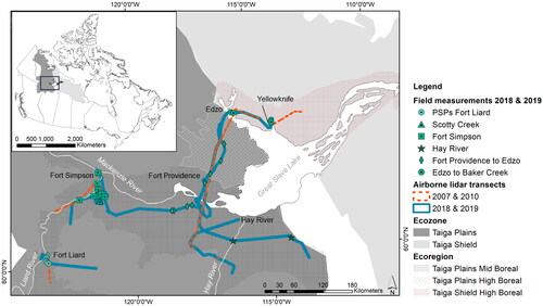
The study was conducted in the southern Taiga, Northwest Territories, Canada, underlain by sporadic to discontinuous permafrost (Figure 1) across a latitudinal range of 500 km and a longitudinal range of 300 km. The terrain of the study region is gently undulating to level. In the Taiga Plains Mid Boreal, mean elevation decreases from 350 m above sea level in the west (Liard Upland) to 175 m above sea level in the east (Great Slave Lowland). Elevation increases in the Taiga Sield High Boreal from west to east from 100 m to 300 m above sea level. The proportional area per ecosystem type varies across this region along a west to east gradient, whereby up to 71% of the Taiga Plains Mid Boreal ecoregion are covered by peatland complexes and up to 53% and 30% of the Taiga Plains and Taiga Shield High Boreal are covered by extensive shoreline fens around shallow ponds (Ecosystem Classification Group 2008, 2009). Upland mixed-wood, deciduous, and coniferous forests are most productive in the Liard Plain (western Taiga Plains Mid Boreal) and transition to dominantly jack pine (Pinus banksiana) or white spruce (Picea glauca) stands in the fire prone Taiga Plains High Boreal, and jack pine, black spruce (Picea mariana), and paper birch (Betula papyrifera) stands on and between bedrock outcrops in the Taiga Shield High Boreal. Within the extensive peatland complexes in the Taiga Plains Mid Boreal, peat plateaus underlain by permafrost (herein ‘permafrost plateaus’) occur adjacent to lower-lying permafrost-free peatlands. These consist of sparse and stunted black spruce trees with lichen ground cover. The dominant vegetation in peatlands ranges from moss, sedge, and shrub (e.g. dwarf birch (Betula spp.), willow (Salix spp.)) dominated (open) to treed (black spruce and tamarack (Larix laricina)) (Ecosystem Classification Group 2009).

Figure 1. Study area of 2018, 2019 field measurements and airborne lidar transects in the Taiga Plains and Taiga Shield ecozones, Northwest Territories, Canada. Field measurements were used to develop aboveground biomass models based on the coincident 2018, 2019 Titan lidar data. Models were then transferred to the 2007, 2010 ALTM 3100 lidar data. (Ecozone and ecoregion boundaries were derived from the National Ecological Framework for Canada dataset).

Field measurements

Field data were collected from mid-July to mid-August in 2018 and 2019 within 53 transects of approximately 25 m in length (Flade et al. 2020, 2021). Transects were sampled in unmanaged ecosystems undisturbed by insect infestation with some in areas burned by wildland fire (<70 years). Transects started in forested uplands or permafrost plateaus and traversed into adjacent peatlands perpendicular to the outer transition boundary at ∼10 m along each transect. Outer transition boundaries were visually determined where forests noticeably reduced in plant height and changed in species composition from trees mixed with shrubs and herbaceous vegetation into moss, grass, sedge, and shrub dominated “open peatlands” or sparsely forested “treed peatlands”.

Measurements were made within circular forest mensuration plots (5 m radius, 78.5 m²; n = 36) installed at the start of the transect and included genus/species identification, tree density, tree height (Vertex 5 Haglöf Sweden) and stem diameter at the base (tree height <1.5 m) and at breast height for every live tree. Typical forest mensuration plots span a 400 m² area. However, due to prioritizing the amount of transects across the region over the size of forest mensuration plots, we reduced the area to encompass a 5 m radius around the center point of the transect start. Plots included between 14 and 76 individual trees (average 40), representing a range of structural characteristics. Transect start and end points were located using Global Navigation Satellite System (GNSS) Hiper SRII base station and rover (Topcon Corp., Japan). Surface level measurements of ground elevation were collected at 1 m intervals along the transect to ensure accurate registration with airborne lidar data. Plant structural data were collected within 1 m² plots (herein ‘micro plots’) along the transect (n = 1250). Measurements included two-dimensional cover and height for live woody short-stature (≤4.5 m) to tall-stature (>4.5 m) plants per genus/species (Flade et al. 2020, 2021).

In addition to transects, field data from 20 permanent sampling plots (PSPs) in upland forests near Fort Liard were used to increase the representation of the upper range of tall-stature tree AGB in our study area (Figure 1). Precise Point Positioning (PPP) GNSS measurements were used to geolocate two diagonal corners of each of the 400 m² rectangular plots, operated for ∼ 45 minutes at each corner to converge to centimetre-grade accuracy. Measurements consisted of tree height and diameter at breast height (DBH) for short-stature (DBH <9 cm) and tall-stature trees (DBH ≥9 cm). Species-level shrub cover and 1 out of 3 height categories were also collected. Shrub species were assigned the average height value of the respective height category. For ground covering shrub species, we determined height based on the average height of the respective species as measured in proximal transect vegetation plots. The selection of PSPs limited to Fort Liard (where upland forests are most productive) was due to the availability of highly accurate geo-located field data coincident to Titan lidar data (described below), which was not available at other PSP locations within the NWT. In addition, these sites were visited in person enabling a better understanding and documentation of vegetation structure and composition as well as site condition.

Field-based aboveground biomass derivation

To determine short-stature (≤4.5 m height) plant AGB within each plot, the product of cover and height per shrub genus/species resulted in a three-dimensional volume derivative, which was used as input into genus/species-specific shrub allometric equations based on iterative nonlinear least squares regression (Flade et al. 2020). Short-stature tree stem length served as input into genus/species-specific tree allometric equations using iterative nonlinear least squares regression (Table 1, Flade et al. 2020). For shrub and short-stature tree genera/species without a dedicated allometric equation, the pooled allometric equations for shrubs, soft, and hardwood trees were used (Flade et al. 2020). For tall-stature tree species, tree height and diameter at breast height (DBH) were used in allometric AGB equations provided by Lambert et al. (2005).

Table 1. Stem length-based regression coefficient estimates with error statistics to be input into Equation (4)–(7) (Flade et al. 2020) for linear logarithmic regression with correction (LLRC) and iterative nonlinear least squares regression (NLS) as appropriate to derive short-stature tree AGB (≤4.5 m height).

		Coefficients
		LN(β)	β	SE (β)	α	SE (α)	CF	R^2 (%)	RMSE (g)
Betula papyrifera	LLRC	2.485	12.0010		2.7300		1.0764	89.8	65.41
	NLS		3.9337	2.5136	3.9470	0.5440		92.5	44.93
Picea glauca	LLRC	4.938	139.4910		2.2640		1.0405	81.0	471.04
	NLS		242.6640	117.9150	1.7489	0.3940		82.7	414.62
Picea mariana	LLRC	5.131	169.1862		2.1910		1.1047	70.7	464.89
	NLS		282.5400	118.1550	1.6753	0.3920		73.7	413.48
Populus balsamifera	LLRC	2.897	18.1197		2.0780		1.0722	91.4	31.02
	NLS		20.8387	4.2502	2.0616	0.1698		91.4	30.33
Populus tremuloides	LLRC	2.429	11.3475		2.2790		1.0824	88.4	32.01
	NLS		6.1033	1.6867	2.9998	0.2316		91.0	25.42
Softwood (Picea spp.)	LLRC	5.041	154.6246		2.2240		1.0775	76.6	488.66
	NLS		268.9470	79.7794	1.6831	0.2526		79.1	415.77
Hardwood	LLRC	2.691	14.7464		2.1960		1.1054	79.3	54.92
	NLS		13.2239	3.1752	2.4982	0.2020		79.5	51.31
Multi-species trees	LLRC	3.366	28.9624		2.1320		1.9117	28.5	484.83
	NLS		45.8224	28.8121	2.3799	0.5261		28.6	482.77

SE: Standard error; CF: correction factor.

Finally, AGB for each plant was summed within forest mensuration and micro plots for comparison with airborne lidar data. Further aggregation of field-based AGB was conducted to ensure adequate numbers of lidar returns per plot required for lidar return metric comparisons with field-based AGB. Micro plots along transects were aggregated separately within forested areas including transition zones and peatlands, and summed AGB in forests (including transition zone) and peatlands were scaled to 2 m widths. For circular forest mensuration plots that overlapped with the micro plots, we scaled the summed shrub AGB (forests including transition zone) to the same area as the forest mensuration plots and added the two AGB amounts together. Total AGB was converted to Mg ha⁻¹, resulting in 59 forest (including transition zones) and 44 peatland AGB values which were compared in a regression analysis with airborne lidar return metrics.

Airborne lidar data collection and processing

Airborne lidar surveys were conducted between July 30th to August 3rd, 2007, and 2010 and again during July and August of 2018 and 2019 coincident with field data collection. Lidar systems used were small-footprint multiple-discrete return Teledyne Optech Inc. (Ontario, Canada) Airborne Laser Terrain Mappers (ALTM). In 2007 and 2010, an ALTM 3100 system (manufactured in 2004) was used operating at 1064 nm wavelength, while in 2018 and 2019 surveys were conducted with an ALTM Titan multi-channel system (manufactured in 2015) operating in three wavelengths (532 nm, 1064 nm and 1550 nm). Both were operated with similar flight and sensor settings, but the newer Titan sensor produced two to three times the return density of the older system (Table 2).

Table 2. Lidar survey settings and configuration of the single channel ALTM 3100 and multi-channel Titan sensors.

Sensor model	ALTM 3100	Titan
Dates of surveys	Jul/Aug 2007, 2010	Jul/Aug 2018 & 2019
Wavelength (nm)	1064	532, 1064, 1550
Pulse repetition frequency (kHz)	50–70	75–100 (225–300 total)
Field of view (deg)	30–40	30
Flying altitude (m agl)	∼900–1500	∼900–1200
Nominal point density (pts/m^2)	∼3	∼8
Approximal horizontal (x, y) and vertical (z) offsets to ground control (Titan) and between data sets	<1m (x, y) and <0.3 m (z)

Following pre-processing, the 3D lidar point clouds were quality controlled and filtered using TerraScan (Terrasolid Ltd., Finland). Low, air points, and isolated returns (noise) were deleted for quality control purposes, and remaining single and last returns were classified into ground points. All returns within −0.1 m to 0 m vertical distance to ground points were added to the ground class. All remaining non-ground returns were normalized relative to height above ground using ‘LASheight’ within the LAStools suite (rapidlasso GmbH, Germany).

To mitigate long GNSS baseline trajectory errors and facilitate accurate comparisons between the Titan lidar data and coincident field plot and transect data, lidar point clouds were manually block adjusted (per lidar flight strip) in x, y, and z direction to match ground control. Where necessary, adjustments in x, y, and z were made for each surveyed transect by overlapping the Titan lidar point clouds in Quick Terrain Modeler (version 8.3.1, Applied Imagery, USA) with ground control points (Profile Analysis Tool) and visually adjusting the Titan lidar data until systematic differences were reduced to zero. Control points and other visual reference data consisted of 1 m interval ground surface elevations (GNSS and surface leveling measurements) and localized maximum short-stature and tall-stature vegetation heights. For all field transects and lidar flight strips the required adjustments were <1 m in x and y and <0.3 m in z (Table 2). Ground classified lidar data from 2007 and 2010 ALTM 3100 surveys were then registered to the aligned Titan lidar data by again overlapping the point clouds and shifting the ALTM 3100 data. Offsets were within the range mentioned above (Table 2).

Registered and height normalized returns were then clipped to coincident field transects (forests including transition zone, and peatlands) and forest-mensuration plots for regression and model development. Common lidar metrics were derived for each clipped area using LAStools and the “lidR” package (Roussel et al. 2020; Roussel and Auty 2022) (R Core Team 2021, Austria). These included height percentiles (from the 5th to the 99th percentile), interquartile range of return heights (25th to 75th height percentile), minimum, maximum, average, and standard deviation of all heights, kurtosis, skewness, and average square height using all lidar returns above ground level (hagl). Cover and density metrics were derived for all lidar returns above 0.5 m hagl. Lidar metrics per sensor were also gridded at 5 m × 5 m grid cell resolution for the complete region (“lidR” and “raster” packages in R) to apply the final AGB model. This cell size was chosen to ensure sufficient numbers of points per Titan and ALTM 3100 grid cell (needed to distinguish between lidar height percentiles), while also maintaining relatively high spatial resolution. This is especially important in ecotones that may be changing horizontally but are within a Landsat grid cell. 5 m cells can also be aggregated to the scale of forest inventory plots (typically 20 m × 20 m or 11.28 m radius, National Forest Inventory) and Landsat imagery (30 m × 30 m grid cell). A canopy height model was derived at the same grid cell resolution based on the maximum height of each cell.

Lidar-based aboveground biomass model development

Correspondence between coincident field-derived AGB and lidar metrics per clipped area was evaluated within a pre-selection process using the Pearson correlation coefficient, retaining those metrics that had the highest or second highest correlations in a minimum of two strata. Furthermore, lidar metrics were retained when assumptions of parametric regression were met, as tested by the Anderson Darling test to determine deviation of residuals from normality, as well as residual plots to determine heteroscedasticity. Each of the remaining lidar metrics was used as the predictor variable within single variable iterative nonlinear least squares regression via a power function (Equation (1)(1) $${\mathit{\text{AGB}}}_{\mathit{\text{lidar sensor}}}=b*{\mathit{\text{lidar metric}}\mathrm{ }}^a$$(1) ), which is commonly used to infer AGB from field and lidar data. The model form was: (1) $${\mathit{\text{AGB}}}_{\mathit{\text{lidar sensor}}}=b*{\mathit{\text{lidar metric}}\mathrm{ }}^a$$(1) where $b$ and $a$ are model coefficients. To better understand magnitudes of model errors of nonlinear least squares regression, model fits were compared to linear regression with forced y-intercept. Forcing the intercept through the origin ensured that AGB equaled zero for zero lidar points above the terrain surface. Model performance per lidar metric was analyzed to determine the optimal lidar metric for (1) each stratum (ecozone, ecosystem type) and (2) all strata combined using leave-one-out cross validation during model development. Goodness-of-fit statistics included the coefficient of determination (R²), root mean squared error (RMSE), and absolute model bias (Bias) which are most commonly used in AGB regression analysis (Coops et al. 2021). To compare RMSEs across strata that deviate in their group means, the root mean squared error and bias relative to the mean (RMSE% and Bias% respectively) were derived.

To determine whether a single lidar metric could be used to model AGB with moderate to high accuracy across the region, a general AGB model was developed for each lidar metric using data of all strata combined (herein called ‘general AGB model’). To evaluate model accuracies, the general AGB models (one for each lidar metric) were applied to each stratum and compared to respective stratum-specific AGB model fits.

The criteria for the selection of the optimal lidar metric as predictor of bi-temporal shrub-to-tree AGB required: (1) high goodness-of-fit statistics of the general AGB model for each stratum, and (2) minimal difference in the lidar metric when compared between sensors (see below).

Lidar metric comparison across sensors

When transferring an AGB model trained for Titan to the older ALTM 3100 data, systematic errors might occur due to differences in point cloud density (Lim et al. 2008) or canopy penetration characteristics (Chasmer et al. 2006; Hopkinson 2007) even when flight settings and sensor calibration are the same between flights and point clouds are geo-registered. To test for deviations between the sensors’ characterizations of height without available corresponding field data, deviations had to be isolated from signals stemming from successional vegetation changes. Therefore, gridded lidar metrics were compared between sensors in late-successional upland forests in which canopy characteristics between the two survey periods (8–12 years) were assumed to be minimal due to slow successional changes in the study region (Castilla et al. 2022). This assumption was corroborated by observed negligible changes in the ALTM 3100 and Titan 5 m × 5 m Canopy Height Models combined with qualitative comparisons at matching locations in Google Earth Pro where multi-year imagery was available. Hereby, general areas of stable maximum canopy height in uplands were visually identified for sample locations across the entire study region. Within these, a total of 558 grid cells were randomly selected at which values of lidar metrics were extracted for further model transfer analysis. To confirm negligible change in these grid cells, differences in mean canopy height and standard deviation were quantified. Differences in the first quartile (based on the distribution of extracted canopy heights) were also determined to test for negligible changes in short-stature vegetation as found in the forest understory or in open upland sites. Subsequently, to quantify deviations between the sensors’ characterizations of height, the covariance of each corresponding Titan (observed) and ALTM 3100 (predicted) lidar metric was derived for sampled grid cells by comparing the slope against the 1:1 line of correspondence between observed and predicted values (Piñeiro et al. 2008). Lidar metrics retained as candidates for the final bi-temporal shrub-to-tree AGB model development were selected based on demonstrating ≤ ±2% deviation from unity (1:1) in slope and ≥95% in explained variance (R²).

Lidar metric calibration and selection for bi-temporal shrub-to-tree aboveground biomass modeling

Based on the two criteria of high goodness-of-fit statistics across strata for the general AGB models and high covariance between corresponding Titan and ALTM 3100 lidar metrics, the retained ALTM 3100 lidar metrics were calibrated using the slope (determined above) as calibration coefficient ($c$, Equation (2)(2) $${\mathit{\text{AGB}}}_{\mathit{\text{ALTM}}\mathrm{ }3100,\mathit{\text{calibrated}}}=b*{\left(c*\mathit{\text{lidar metric}}\right)}^a.$$(2) ). General ALTM 3100 AGB was subsequently modeled for each grid cell per lidar metric as: (2) $${\mathit{\text{AGB}}}_{\mathit{\text{ALTM}}\mathrm{ }3100,\mathit{\text{calibrated}}}=b*{\left(c*\mathit{\text{lidar metric}}\right)}^a.$$(2)

General Titan AGB per grid cell was derived without the application of a calibration coefficient (Equation (1)(1) $${\mathit{\text{AGB}}}_{\mathit{\text{lidar sensor}}}=b*{\mathit{\text{lidar metric}}\mathrm{ }}^a$$(1) ).

Finally, for the selection of the optimal predictor of bi-temporal shrub-to-tree AGB, deviations in modeled general Titan and calibrated ALTM 3100 AGB were analyzed across lidar metrics to identify AGB ranges for which lidar metrics deviated in their predictions. This comparison was based on 1381 sampled grid cells distributed randomly across the study region, which covered AGB values from 0 to 400 Mg ha⁻¹. A recommendation for the optimal lidar metric was made relative to a specific AGB range. The final bi-temporal shrub-to-tree AGB model was then a combination of metrics applied to specific AGB ranges using a weighted approach. Hereby, modeled AGB per lidar metric (herein called exemplarily ‘model output 1’ and ‘model output 2’) was multiplied by a weighting factor (0%–100%), which increased for model output 1 and decreased inversely for model output 2 as a certain AGB range was approached for which model output 1 was deemed more reliable (i.e. lower variance in AGB compared between sensors).

Results

Aboveground biomass model comparison

A comparison of the field-based AGB across strata is illustrated in Table 3 to provide geographic context for the distribution across ecozones and ecosystem types. Field data indicated that the Taiga Plains contained more than three times the average AGB as found in the Taiga Shield. However, some data were collected in highly productive forests near Fort Liard (Figure 1), resulting in a shift in the third quartile. Within ecosystem types, forests in uplands and permafrost plateaus also contained greater average biomass relative to peatlands, which are commonly dominated by ‘open’ moss and graminoid forms.

Table 3. Descriptive statistic of field-derived AGB (Mg ha⁻¹) for the complete field data and stratified into ecozone and ecosystem type.

Strata	n	Mean (SD)	1st Quartile	3rd Quartile	Max
All ecosystem types and ecozones	103	49.9 (75.2)	2.3	54.1	330.4
Ecozone
Taiga Plains	79	65.7 (85.3)	4.0	118.4	330.4
Taiga Shield	24	17.0 (18.6)	0.8	30.9	56.6
Ecosystem type
Upland/Permafrost plateau forests	59	96.0 (85.2)	29.5	143.6	330.4
Peatlands	44	3.9 (5.4)	0.7	4.1	21.8

SD: Standard deviation.

The lidar metrics retained in the pre-selection process were characteristic of the height distributions of lidar returns consisting of the average height, interquartile range of heights, and 75th and 90th height percentiles of all lidar returns within each plot (Table 4). In addition, we included the 95th height percentile, which is a common predictor of canopy height (Mahoney et al. 2018; Popescu et al. 2002; Riggins et al. 2009) and growth in forests (Hopkinson et al. 2008).

Table 4. Pearson correlation coefficient of linear relationships between Titan lidar metrics and field-based AGB within corresponding plots used to refine the selection of lidar metrics for lidar-based stratum specific and general AGB model development.

	Taiga Plains	Taiga Shield	Upland/Permafrost plateau forests	Peatlands	All data
Percentile 5	−0.23	0.00	−0.18	0.55	−0.14
Percentile 10	−0.13	0.00	−0.07	0.55	−0.03
Percentile 25	0.59	0.12	0.56	0.55	0.66
Percentile 50	0.90	0.33	0.89	0.61	0.93
Percentile 75	0.95	0.74	0.92	0.78	0.97
Percentile 90	0.94	0.79	0.90	0.57	0.95
Percentile 95	0.93	0.72	0.89	0.43	0.94
Percentile 99	0.91	0.71	0.87	0.40	0.92
Interquartile range	0.94	0.74	0.91	0.76	0.96
Average height	0.95	0.76	0.92	0.69	0.97
Average square height	0.89	0.68	0.86	0.43	0.92
Minimum	−0.23	0.00	−0.18	0.55	−0.15
Maximum	0.89	0.68	0.85	0.33	0.90
Standard deviation	0.94	0.74	0.90	0.43	0.95
Cover (> 0.5 m hagl)	0.80	0.66	0.75	0.71	0.78
Density (> 0.5 m hagl)	0.83	0.71	0.79	0.66	0.81
Kurtosis	−0.39	−0.50	−0.45	−0.24	−0.38
Skewness	−0.60	−0.52	−0.68	−0.22	−0.57

Highest Pearson correlation coefficient per stratum colored in grey, second highest colored in yellow.

Using each of these lidar height metrics (m hagl) as input variable within nonlinear least squares regression via a power function resulted in moderate to high correspondence to field-derived AGB (Mg ha⁻¹) for stratum specific models (R² = 61% to 90% reported for the best lidar height metric per stratum) (Table 5). Model errors were moderate overall for highest R² predictors (RMSE < 34 Mg ha⁻¹; Bias < 26 Mg ha⁻¹) but were greater in peatlands and the Taiga Shield ecozone. Model errors increased for all strata and lidar metrics using the linear model form (difference in RMSE% = 0–21; difference in Bias% = −4 to 7) (Table 5).

Table 5. Titan lidar height metrics after pre-selection, regression coefficients and leave-one-out cross validated model fits for stratum-specific and general AGB models using single variable nonlinear least squares regression via a power function.

	Coefficients
Lidar metric	b	SE (b)	a	SE (a)	R^2 (%)	RMSE (Mg ha^−1)	RMSE (%)	Bias (Mg ha^−1)	Bias (%)
General model
Average height	21.974	1.951	0.966	0.038	93.7	18.9 (+0.8)	38.0 (+1.5)	12.8 (-0.1)	25.7 (−0.1)
IQR	14.969	1.822	0.939	0.440	92.0	21.4 (+1.0)	42.8 (+2.1)	13.6 (0)	27.4 (0)
Percentile 75	12.979	1.510	0.966	0.041	93.7	19.0 (+0.7)	38.2 (+1.3)	12.7 (0)	25.4 (0)
Percentile 90	5.393	0.950	1.187	0.058	91.4	22.0 (+1.9)	44.1 (+3.8)	13.9 (+1.2)	27.8 (+2.4)
Percentile 95	3.346	0.724	1.306	0.070	72.9	24.0 (+3.6)	48.2 (+7.1)	14.8 (+3.4)	29.6 (+6.8)
Taiga Plains model
Average height	27.084	3.170	0.890	0.051	90.0	27.0 (+1.5)	41.2 (+2.2)	18.4 (−0.8)	28.0 (−1.2)
IQR	19.493	2.986	0.856	0.056	88.7	27.4 (+3.3)	41.7 (+5.0)	18.8 (+0.1)	28.6 (+0.2)
Percentile 75	17.214	2.655	0.878	0.055	89.8	28.7 (0)	43.7 (0)	18.1 (−0.2)	27.5 (−0.2)
Percentile 90	7.644	1.636	1.083	0.071	88.5	28.9 (+0.9)	44.0 (+1.4)	19.3 (+0.2)	29.4 (+0.3)
Percentile 95	5.088	1.285	1.183	0.082	87.2	30.6 (+1.9)	46.5 (+2.8)	20.6 (+2.0)	31.4 (+3.0)
Taiga Shield model
Average height	23.524	3.094	0.706	0.183	61.2	11.6 (+1.1)	68.4 (+6.2)	8.3 (−0.3)	48.6 (−1.6)
IQR	21.315	3.020	0.493	0.112	64.9	11.1 (+3.0)	65.0 (+17.8)	8.6 (−0.7)	50.7 (−3.8)
Percentile 75	21.067	3.049	0.495	0.114	64.3	11.2 (+2.9)	65.6 (+17.2)	8.7 (−0.7)	51.0 (−4.3)
Percentile 90	10.629	3.512	0.718	0.207	64.0	11.2 (+0.9)	65.6 (+5.2)	7.2 (+0.2)	42.5 (+1.0)
Percentile 95	9.008	3.874	0.673	0.238	55.4	12.5 (+1.4)	73.2 (+8.4)	7.7 (-0.6)	45.2 (−3.5)
Upland/Permafrost plateau forest model (including ecotones)
Average height	32.744	4.203	0.811	0.058	84.5	33.5 (+3.2)	34.9 (+3.3)	25.8 (+0.1)	26.8 (+0.1)
IQR	22.037	3.770	0.813	0.064	82.3	36.0 (+2.9)	37.5 (+3.1)	28.2 (+0.7)	29.4 (+0.7)
Percentile 75	20.578	3.542	0.817	0.062	83.5	34.7 (+2.6)	36.2 (+2.7)	27.2 (+0.3)	28.4 (+0.3)
Percentile 90	10.069	2.371	0.995	0.080	81.8	36.4 (+0.6)	37.9 (+0.6)	28.2 (0)	29.4 (0)
Percentile 95	7.432	2.044	1.064	0.091	79.8	38.3 (+0.8)	39.9 (+0.8)	29.3 (+0.3)	30.5 (+0.4)
Peatland Model
Average height	11.492	1.260	1.410	0.270	51.0	3.8 (+0.3)	98.3 (+8.0)	2.5 (+0.1)	65.0 (+2.8)
IQR	11.136	1.090	0.776	0.116	56.3	3.6 (+0.3)	92.3 (+8.7)	2.4 (0)	61.1 (−1.0)
Percentile 75	9.803	0.911	0.865	0.122	61.1	3.4 (+0.2)	87.0 (+6.3)	2.4 (−0.1)	60.9 (−1.8)
Percentile 90	4.229	0.931	0.703	0.218	31.9	4.5 (+0.3)	115.1 (+9.0)	2.9 (0)	75.4 (−1.0)
Percentile 95	3.573	0.897	0.503	0.190	23.7	4.7 (+0.8)	122 (+20.5)	3.0 (0)	78.8 (−1.0)

Comparison to increased (+) and decreased (−) model errors of linear regression with forced y-intercept in brackets.

SE: Standard error, IQR: interquartile range. Highest goodness-of-fit metrics per stratum colored in grey.

Comparisons of goodness-of-fit statistics across lidar height metrics showed that average height was the best predictor of field-derived AGB for the Taiga Plains and upland/permafrost plateau forests (R² = 90% and 85%; RMSE = 27 Mg ha⁻¹ and 34 Mg ha⁻¹ respectively). For the remaining strata, model fits improved using the interquartile range as predictor variable within the Taiga Shield model (R² = 65%; RMSE = 11 Mg ha⁻¹), and the 75^th height percentile within the peatland model (R² = 61%; RMSE = 3 Mg ha⁻¹).

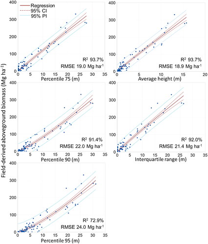
Model performance improved when modeling AGB for all strata combined using the general AGB model (R² = 73%–94%, RMSE = 19 Mg ha⁻¹–24 Mg ha⁻¹, Bias = 13 Mg ha⁻¹–15 Mg ha⁻¹) (Table 5). Highest correspondence to field-based AGB and lowest model errors were hereby achieved using the average height or the 75th height percentile as predictor variable (R² = 94%; RMSE = 19 Mg ha⁻¹; Bias =13 Mg ha⁻¹) (Figure 2).

Figure 2. Field-derived aboveground biomass (AGB) related to lidar height metrics (m) for all strata combined using iterative nonlinear least squares regression via a power function illustrated within the 95th confidence interval (CI) and 95th prediction interval (PI).

Evaluating the performance of the general AGB models (developed per lidar height metric) within each stratum (Table 6) showed a mean reduction in explained model variability by −2% and a mean increase in RMSE by 1 Mg ha⁻¹, while Bias remained stable in average at 0.3 Mg ha⁻¹. Magnitudes of decreased model performance varied per ecosystem type and lidar metric used. In the Taiga Plains and upland/permafrost plateau forests, the predictor average height produced highest model fits (R² = 90% and 84%; RMSE = 28 Mg ha⁻¹ and 36 Mg ha⁻¹ respectively). In the Taiga Shield, explained model variance was highest for the 90th height percentile (R² = 59%), while model errors were lowest for the average height (RMSE = 12 Mg ha⁻¹; Bias = 8 Mg ha⁻¹). In peatlands, the 75th height percentile explained the highest model variance (R² = 61%) and had lowest model errors (RMSE = 4.0 Mg ha⁻¹; Bias = 2.6 Mg ha⁻¹). However, relative to the measured mean, AGB model errors where high (RMSE% = 103; Bias% = 67).

Table 6. General AGB model fits per Titan lidar height metric evaluated for stratum-specific Taiga ecoregions and ecosystem types.

Lidar metric	R^2 (%)	RMSE (Mg ha^−1)	RMSE (%)	Bias (Mg ha^−1)	Bias (%)
Taiga Plains
Average height	89.7	27.7 (+0.3)	42.2 (+0.5)	17.7 (+0.1)	27.0 (+0.1)
IQR	88.6	29.3 (+0.6)	44.6 (+1.0)	18.4 (+0.3)	28.1 (+0.4)
Percentile 75	89.7	28.0 (+0.3)	42.6 (+0.5)	17.6 (+0.1)	26.8 (+0.2)
Percentile 90	86.9	29.5 (0)	45.0 (0)	19.8 (−0.4)	30.2 (−0.6)
Percentile 95	86.9	31.2 (+1.0)	47.6 (+1.5)	19.8 (+2.6)	30.2 (+3.9)
Taiga Shield
Average height	57.9	12.3 (0)	72.0 (+0.1)	8.2 (−0.2)	48.0 (−1.0)
IQR	56.6	14.0 (+0.2)	82.2 (−1.1)	9.1 (-0.6)	53.4 (−3.3)
Percentile 75	55.8	13.6 (0)	79.7 (+0.2)	8.5 (−0.4)	50.1 (−2.1)
Percentile 90	59.4	12.4 (+2.1)	72.7 (+12.4)	8.2 (+2.1)	48.2 (+12.3)
Percentile 95	47.5	14.8 (+5.2)	87.1 (+30.4)	8.5 (+4.0)	49.7 (+23.7)
Upland/Permafrost plateau forest (including ecotones)
Average height	84.1	35.9 (+0.7)	37.4 (+0.7)	25.6 (+0.6)	26.7 (+0.6)
IQR	82.5	37.4 (+1.1)	39.0 (+1.1)	28 (+0.5)	29.1 (+0.5)
Percentile 75	83.8	36.6 (+0.6)	38.1 (+0.6)	27 (+0.3)	28.1 (+0.3)
Percentile 90	81.6	38.3 (−1.3)	39.9 (−1.3)	28 (−0.5)	29.2 (−0.5)
Percentile 95	79.5	40.7 (−1.3)	42.3 (−1.3)	29.2 (0.4)	30.4 (+0.4)
Peatland
Average height	47.5	7.1 (−0.8)	183.3 (−19.9)	5.0 (−0.7)	129.3 (−17.1)
IQR	57.0	4.2 (−0.4)	108.4 (−10.0)	2.6 (−0.2)	66.3 (−4.7)
Percentile 75	61.4	4.0 (−0.3)	102.5 (−7.1)	2.6 (−0.1)	66.6 (−3.4)
Percentile 90	32.5	6.8 (+3.6)	175.4 (+92.2)	3.9 (+2.3)	101.8 (+60.4)
Percentile 95	14.2	10.7 (+6.4)	278.0 (+165.6)	5.2 (+5.2)	135.2 (+134.2)

Interquartile range (IQR). Highest goodness-of-fit metrics per stratum colored in grey.

Comparison to increased (+) and decreased (−) model errors of linear regression with forced y-intercept in brackets.

Lidar metric comparison across sensors

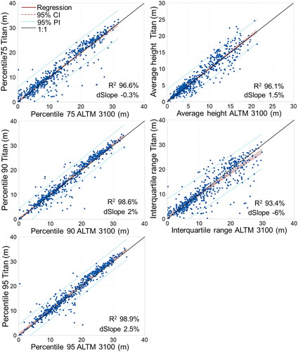
To identify the optimal lidar height metric candidates for predicting bi-temporal shrub-to-tree AGB, the second criteria (besides high goodness-of-fit statistics for each stratum) required negligible, calibratable systematic error when transferring the model trained for the Titan data to older ALTM 3100 data. To isolate sensor differences from signals stemming from successional vegetation changes, 558 grid cells in late-successional upland forests were selected and analyzed. Here, differences in the mean canopy height were within ± 0.5 m and differences in the standard deviation ranged from 0 to 0.4 m for the retained lidar metrics. Differences in the first quartile were within ± 0.1 m (except for the 95th height percentile and the interquartile range ± 0.5 m) representative of short-stature vegetation found in the understory and in open upland sites. Evaluation of covariance between Titan and ALTM 3100 lidar height metrics in these late-successional upland sites showed lowest overall explained variance and highest deviations from a 1:1 linear relationship for the interquartile range and the 95^th height percentile, which in addition to lowest goodness-of-fit statistics excluded them from subsequent bi-temporal shrub-to-tree AGB model development Table 7.

Table 7. Covariances between corresponding multi-channel Titan (observed) and single channel ALTM 3100 (predicted) lidar height metrics.

Lidar metric	Calibration coefficient $c$	SE of calibration coefficient $c$	R^2
General AGB model
Average height	1.0149	0.0086	96.1
IQR	0.9405	0.0106	93.4
Percentile 75	0.9969	0.0079	96.6
Percentile 90	1.0200	0.0051	98.6
Percentile 95	1.0253	0.0046	98.9

Calibration coefficients $c$ represent the slope of the linear relationship between observed and predicted lidar height metrics. These were used to correct the respective ALTM 3100 height grids for subsequent use in the bi-temporal shrub-to-tree AGB model (Equation (3)(3) $$\begin{array}{c}\mathit{\text{AG}}{B}_{\left(\mathit{\text{Titan}};\mathit{\text{calibrated ALTM}}\hspace{0.17em}3100\right)}=x\text{*}\mathit{\text{AG}}{B}_{\mathrm{average\; heigh}\text{t}}+\\ y\text{*}\mathit{\text{AG}}{B}_{90\mathit{\text{th height}}\hspace{0.17em}\mathit{\text{percentile}}}\hspace{0.17em}\end{array}$$(3) ).

SE: Standard error; IQR: interquartile range.

The lowest deviations across sensors were achieved for the 75th height percentile (difference in slope compared to 100% = −0.3%) (Table 7). However, correspondence between the Titan and ALTM 3100 75th height percentiles showed increased variance toward higher Titan values below 3 m (Figure 3). For vegetation heights below 5 m, lowest variances were achieved by the average height (Figure 3). The 1.5% difference in slope (relative to 100%) for the complete average height range is driven by increased variances for average heights above 10 m. Here, the 90th height percentile showed lower variance (Figure 3) resulting in the highest overall correspondence between sensors (R² = 99%) albeit deviations from a 1:1 slope by 2%.

Figure 3. Covariance of Titan (observed) and ALTM 3100 (predicted) lidar height metrics to evaluate potential for systematic error during aboveground biomass model transfer based on 558 randomly selected grid cells in late successional upland forests. Slopes are represented as percent deviation of a 1:1 relationship (dSlope).

For further development of the bi-temporal shrub-to-tree AGB model, ALTM 3100 lidar metrics were calibrated using the slope (Table 7) as calibration coefficient (Equation (2)(2) $${\mathit{\text{AGB}}}_{\mathit{\text{ALTM}}\mathrm{ }3100,\mathit{\text{calibrated}}}=b*{\left(c*\mathit{\text{lidar metric}}\right)}^a.$$(2) ).

Lidar metric selection for bi-temporal shrub-to-tree aboveground biomass model development

For selecting the optimal lidar height metric as predictor of bi-temporal shrub-to-tree aboveground biomass, both goodness-of-fit statistics of modeled AGB (general AGB model per height metric) (Table 6) and covariance of corresponding lidar metrics between sensors (Table 7, Figure 3) revealed the average height, 75th height percentile, and 90th height percentile as the top three candidates. Using the 75th height percentile as predictor, highest goodness-of-fit statistics were achieved for all strata combined (same as average height) and for peatlands while overall deviation in 75^th height percentiles between sensors was negligible. However, the increased variance between sensors for vegetation heights below 3 m (noted above) was critical because this threshold is representative of vegetation heights found dominantly in peatland complexes, potentially overestimating increases in peatland AGB between 2018, 2019 Titan and 2007, 2010 ALTM 3100 lidar surveys. In comparison, the average height metric demonstrated lower variances across sensors for short-stature vegetation and lowest model errors for all strata except peatlands when used as predictor within the general AGB model. In peatlands, model errors exceeded those of the 75th height percentile-based general AGB model, but these were likewise high at RMSE% >100 and Bias% >60. Increased variances in the upper height range across sensors suggested however, that the average height was not the single optimal predictor for the complete AGB range. For upper vegetation heights, the 90th height percentile showed lower variance between sensors and 90^th height percentile-based general AGB model results achieved high goodness-of-fit statistics in uplands/permafrost plateaus (R² = 82%; RMSE = 38 Mg ha⁻¹; Bias = 28 Mg ha⁻¹) (Table 6). This indicated that the optimal lidar metric for modeling bi-temporal shrub-to-tree AGB was a function of the respective AGB range, representative of differences in vegetation structure and canopy heights. 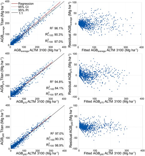Calibration of ALTM 3100 lidar metrics (Equation (2)(2) $${\mathit{\text{AGB}}}_{\mathit{\text{ALTM}}\mathrm{ }3100,\mathit{\text{calibrated}}}=b*{\left(c*\mathit{\text{lidar metric}}\right)}^a.$$(2) ) was therefore necessary to further evaluate variances of modeled AGB (between sensors) compared for the retained lidar metrics for certain AGB ranges. Corresponding to variances in lidar height metrics across sensors in late-successional upland sites, analysis of general Titan AGB and calibrated ALTM 3100 AGB across the complete study region emphasized lower variance below 100 Mg ha⁻¹ when using average height as predictor, and above 100 Mg ha⁻¹ when using the 90th percentile (Figure 4).

Figure 4. Covariance of Titan (observed) and ALTM 3100 (predicted) aboveground biomass (AGB) to evaluate the optimal lidar height metric as predictor of bi-temporal shrub-to-tree AGB across different ecozones, ecosystem types, and ALTM sensors based on 1381 randomly selected grid cells. Residuals of modeled AGB (ALTM 3100) per lidar height metric (average height (average), 75th and 90th height percentile (p75 and p90)) are presented on the right column.

The final bi-temporal shrub-to-tree AGB model combined the average height-based general AGB model and the 90^th height percentile-based general AGB model within a weighted approach as a function of modeled AGB (average height-based general AGB model). Final AGB per grid cell was then derived as (Equation (3)(3) $$\begin{array}{c}\mathit{\text{AG}}{B}_{\left(\mathit{\text{Titan}};\mathit{\text{calibrated ALTM}}\hspace{0.17em}3100\right)}=x\text{*}\mathit{\text{AG}}{B}_{\mathrm{average\; heigh}\text{t}}+\\ y\text{*}\mathit{\text{AG}}{B}_{90\mathit{\text{th height}}\hspace{0.17em}\mathit{\text{percentile}}}\hspace{0.17em}\end{array}$$(3) ): (3) $$\begin{array}{c}\mathit{\text{AG}}{B}_{\left(\mathit{\text{Titan}};\mathit{\text{calibrated ALTM}}\hspace{0.17em}3100\right)}=x\text{*}\mathit{\text{AG}}{B}_{\mathrm{average\; heigh}\text{t}}+\\ y\text{*}\mathit{\text{AG}}{B}_{90\mathit{\text{th height}}\hspace{0.17em}\mathit{\text{percentile}}}\hspace{0.17em}\end{array}$$(3) whereby $x$ = 100%; $y$ = 0% for AGB ≤ 75 Mg ha⁻¹, and $x$ = 0%; $y$ = 100% for AGB ≥125 Mg ha⁻¹. To avoid artifacts at the 100 Mg ha⁻¹ threshold, a sliding scale was applied between 75 Mg ha⁻¹ and 125 Mg ha⁻¹, which decreased successively for increasing average height based AGB ($x$, Equation (3)(3) $$\begin{array}{c}\mathit{\text{AG}}{B}_{\left(\mathit{\text{Titan}};\mathit{\text{calibrated ALTM}}\hspace{0.17em}3100\right)}=x\text{*}\mathit{\text{AG}}{B}_{\mathrm{average\; heigh}\text{t}}+\\ y\text{*}\mathit{\text{AG}}{B}_{90\mathit{\text{th height}}\hspace{0.17em}\mathit{\text{percentile}}}\hspace{0.17em}\end{array}$$(3) ) and inversely increased successively for increasing 90th height percentile based AGB ($y$, Equation (3)(3) $$\begin{array}{c}\mathit{\text{AG}}{B}_{\left(\mathit{\text{Titan}};\mathit{\text{calibrated ALTM}}\hspace{0.17em}3100\right)}=x\text{*}\mathit{\text{AG}}{B}_{\mathrm{average\; heigh}\text{t}}+\\ y\text{*}\mathit{\text{AG}}{B}_{90\mathit{\text{th height}}\hspace{0.17em}\mathit{\text{percentile}}}\hspace{0.17em}\end{array}$$(3) ) using a step size of 2% for each 1 Mg ha⁻¹.

Bi-temporal shrub-to-tree aboveground biomass model evaluation

To evaluate the bi-temporal shrub-to-tree AGB model, correspondence between modeled (Titan) and measured AGB as well as model error were analyzed and compared to the general Titan AGB models based on the average height and the 90^th height percentile. Here, goodness-of-fit statistics were equal to average height-based model fits for the Taiga Shield and peatland strata. This was because maximum AGB values remained below 75 Mg ha⁻¹ (Table 8). For the Taiga Plains and upland/permafrost plateau strata, model fits improved compared to the 90th height percentile-based model and decreased compared to the average height-based model (R² = 89% and 83%; RMSE = 29 Mg ha⁻¹and 37 Mg ha⁻¹ respectively). Across all strata, reduced correspondence was negligible at −1.5% (R² = 92%) in comparison to the average height-based model. Increases in RMSE% and Bias% remained low at 4% and 2% respectively (RMSE = 21 Mg ha⁻¹; Bias = 14 Mg ha⁻¹) (Table 8).

Table 8. Final bi-temporal shrub-to-tree AGB model evaluated for all strata combined and for stratum-specific Taiga ecoregions and ecosystem types.

	R^2 (%)	RMSE (Mg ha^−1)	RMSE (%)	Bias (Mg ha^−1)	Bias (%)
All strata
	92.2	21.03	42.2	13.7	27.5
Taiga Plains
	89.0	28.6	43.62	18.6	28.3
Taiga Shield*
	57.9	12.3	72.0	8.2	48.0
Upland/Permafrost plateau forests (including ecotones)
	82.7	37.3	38.9	27.0	28.1
Peatlands*
	47.5	7.1	183.3	5.0	129.3

AGB was derived combining the modeled Titan average height-based AGB and 90th height percentile-based AGB within a weighted approach as a function of AGB (Equation (3)(3) $$\begin{array}{c}\mathit{\text{AG}}{B}_{\left(\mathit{\text{Titan}};\mathit{\text{calibrated ALTM}}\hspace{0.17em}3100\right)}=x\text{*}\mathit{\text{AG}}{B}_{\mathrm{average\; heigh}\text{t}}+\\ y\text{*}\mathit{\text{AG}}{B}_{90\mathit{\text{th height}}\hspace{0.17em}\mathit{\text{percentile}}}\hspace{0.17em}\end{array}$$(3) ).

* Same as average height based general AGB model per respective stratum (Table 6).

Discussion

The airborne lidar-based AGB models presented here are the first of their kind that were developed across a range of vegetation structures at varying degrees of vertical and horizontal continuity for the northwestern boreal underlain by sporadic to discontinuous permafrost. To address AGB changes in rapidly changing ecosystems such as forest to peatland ecotones, the final bi-temporal shrub-to-tree AGB model had to accommodate conditions of variable vegetation heights, and understory to overstory canopy covers. As such, model errors were expected to be higher in this region compared to models developed for commercial forests with continuous tall-stature tree canopies. However, albeit at the upper limit, model errors were within the range of errors reported in other studies, while correspondence of lidar-based and field-based AGB was often improved. In boreal Canada for example, Margolis et al. (2015) reported model errors ranging from 30 Mg ha⁻¹ to 33 Mg ha⁻¹ (RMSE) and model correspondence from 50% to 65% (R²) for airborne lidar-based AGB in managed upland mixed wood, conifer, and hardwood stands. Their model fits improved for an ecoregion specific model for the central Canadian Shield for conifer stands (R² = 80%; RMSE = 22 Mg ha⁻¹). However, for mixed wood forests in western Canada, model error increased to 35 Mg ha⁻¹ (Margolis et al. 2015). These results are comparable to our best-fitting stratum specific and general AGB models for the Taiga Shield ecozone (R² = 65% and 58%; RMSE = 11 Mg ha⁻¹ and 12 Mg ha⁻¹) and unmanaged upland/permafrost plateau forests distributed across the complete study region (R² = 85% and 84%; RMSE = 34 Mg ha⁻¹ and 36 Mg ha⁻¹) (Table 5). Model fits based on the final bi-temporal shrub-to-tree AGB model were also within the range of Margolis et al. (2015) (R² = 58% and 83%; RMSE = 12 Mg ha⁻¹ and 37 Mg ha⁻¹ for the Taiga Shield and upland/permafrost plateau forests respectively) (Table 8). For managed forest stands in the eastern Canadian boreal, Luther et al. (2019) reported validated airborne lidar-based AGB regression accuracies of 83% (R²) and 24 Mg ha⁻¹ (RMSE). The RMSE% differed from their measured mean by 18%, which is ∼ half of the RMSE% derived in our study when applying the final bi-temporal shrub-to-tree AGB model in unmanaged upland/permafrost plateau forests (Table 8). However, their field-based mean AGB was 1.3 times greater compared to our study and understory vegetation (<2 m) was not included in their modeling approach. AGB model accuracies could not be compared in Canadian peatland ecosystems due to a lack of comparable studies. Reported model errors of treed wetland AGB across all of Canada (RMSE = 22.2 Mg ha⁻¹) in Margolis et al. (2015) for example, were at the upper limit of our field-based AGB (21.8 Mg ha⁻¹, Table 3). However, Räsänen et al. (2020) derived between 45% to 53% explained model variabilities for deciduous shrubs within a fen peatland in northern Finland using multi-source input data within random forest regression. The average height-based stratum specific and general AGB models as well as the final bi-temporal shrub-to-tree AGB model presented in our study were at the upper end of the reported range in peatlands (R² = 51% and 48% respectively) (Tables 5, 6, and 8).

Overall, AGB model accuracies were higher in the Taiga Plains and in upland/permafrost plateau forests compared to the Taiga Shield and peatlands using either stratum-specific models (Table 5) or a generalized AGB model (Tables 6 and 8) independent of the lidar metric used as predictor. These strata are characteristic of short-stature plant dominance and sparse to absent tree cover and as such are closer to the noise level inherent in airborne lidar data. This is because plant canopies close to the ground surface can often not be accurately positioned in height or distinguished from ground points. Sparse, discontinuous vegetation cover has a higher chance of remaining undetected between single laser scan lines. This is increased where lidar campaigns are flown as single strips across the landscape missing additional lidar returns from side overlaps and resulting overall in lower point densities per m². In addition, the decreased travel distance of laser pulses through a short-stature plant canopy in comparison to a tall-stature canopy reduces the possibility of pulse reflections from plant material at varying heights. This reduces the range of vertical height distributions and lidar return densities, with fewer multiple returns (Hopkinson et al. 2005). Differences between lidar height metrics are therefore less pronounced, increasing the uncertainty of height-based lidar metrics in shorter vegetation (Hopkinson et al. 2005).

The choice of the optimal lidar height metric to be used as predictor within the final bi-temporal shrub-to-tree AGB model depended equally on goodness-of-fit statistics and minimal, calibratable offsets between sensors of different lidar point cloud characteristics (point density and canopy penetration). A previous study by Lim et al. (2008) analyzed the effect of lidar point density on canopy heights. The authors suggested that, analogous to statistical sampling, an increase in point density should not lead to a different canopy height sampling distribution because both (low and high return densities) represent a sample of the complete population (canopy). However, a comparison of vertical height profiles between the Titan and a Gemini ALTM (similar to the ALTM 3100) in upland forests by Hopkinson et al. (2016b) showed that the Titan sensor preferentially sampled upper canopy regions due to reflections from 532 nm and 1550 nm channels. Channel-dependent differences in the canopy height sampling distribution were most pronounced between the 25th and 75th height percentiles and decreased for percentiles > 75%. For the upper percentiles (>90%) differences in lidar height profiles were also lowest between the three Titan channels (Hopkinson et al. 2016b). Here, the use of upper percentiles for deriving AGB tends to be relatively stable within the vertical noise and in the case of multi-channel lidar, deeper than average returns from the canopy at 532 nm and 1550 nm tend to balance higher than average returns from the 1064 nm channel (Hopkinson et al. 2016b). This emphasized the use of the 90^th height percentile (calibrated for the ALTM 3100 data) for higher AGB ranges within the bi-temporal shrub-to-tree AGB model. For lower AGB ranges, our results suggest that differences across sensors reduced using an average as opposed to a percentile approach. The average height represents the central tendency (analogous to center of mass) of a vertical profile from the ground to the top of canopy, equally weighing all datapoints in the distribution. As such, this metric is equally sensitive to the tails at the low (ground) or high (top of canopy) end of the overall distribution and is therefore more influenced by open vs. closed canopy conditions. The implicit integration of vegetation height and cover attributes at the grid cell level made this variable a robust predictor across variable vegetation structures and canopy continuity, and therefore an optimal predictor for stratum-specific AGB models and the bi-temporal shrub-to-tree AGB model. The height calibration of the ALTM 3100 dataset (Equation (2)(2) $${\mathit{\text{AGB}}}_{\mathit{\text{ALTM}}\mathrm{ }3100,\mathit{\text{calibrated}}}=b*{\left(c*\mathit{\text{lidar metric}}\right)}^a.$$(2) ) however was necessary as increased heights in the multi-channel 2018, 2019 Titan dataset compared to the single channel 2007, 2010 ALTM 3100 dataset could overestimate vegetation growth in an AGB change detection analysis.

These results will be relevant in future studies aiming to compare different generation lidar systems and for the validation of spaceborne AGB change products. The ALTM 3100 sensor was state-of-the-art technology circa 2005. Therefore, wide area coverage is available for many parts of Canada, USA, Europe, etc. which contributed to the use of this sensor for many baseline vegetation studies. Since circa 2010, there has been a proliferation of new lidar sensor technologies, including the use of multiple single and variable wavelength lidar systems, which produce high pulse repetition frequencies, high sample point densities, and multi-wavelength capability, especially since 2014. Therefore, the need to compare and calibrate between lidar systems for vegetation change from older to newer technologies to understand and quantify change is becoming increasingly important.

Lastly, the bi-temporal shrub-to-tree AGB model was applied using a weighted approach of the gridded Titan and calibrated ALTM 3100 average height and 90th height percentile-based AGB models. This approach was chosen over the use of stratum-specific AGB models. Model performance increased when the model was developed for the respective dominant vegetation structure and canopy openness, ranging from +1% (−1.6 Mg ha⁻¹) in the Taiga Plains to +7% (−1.2 Mg ha⁻¹) in the Taiga Shield and from +2% (−3.8 Mg ha⁻¹) in upland/permafrost plateau forests to +14% (−3.7 Mg ha⁻¹) in peatlands (reported as difference in R² (RMSE) for the best fitting model per stratum). However, the low n in stratum-specific models (Table 3) reduced confidence in model coefficients, which is reflected in larger model coefficient standard errors in comparison to the general AGB models (Table 5). In addition, for application of stratum-specific AGB models, high confidence is required over which grid cells certain models are applied, which requires the use of an external landcover classification. The total error of modeled AGB will then be the combination of errors of (1) the respective AGB model and (2) the landcover classification. Overall accuracies of an external landcover classification in this region range from 73% to 94% (Bourgeau-Chavez et al. 2019) depending on the landcover type, while western parts of our study area were not included. In addition, classification accuracies are often unknown for specific areas where validation data were not available (e.g. Chasmer et al. 2020; Bourgeau-Chavez et al. 2022) or were developed at an earlier/later date resulting in further discrepancies. The compound errors of a combined use of stratum specific AGB models and a static landcover classification are therefore expected to exceed the error of a generalized AGB model. Edge effects at class boundaries will especially be minimized using the bi-temporal shrub-to-tree AGB model enabling investigation of ecotonal changes, which are changing most rapidly with climate change (Chasmer and Hopkinson 2017).

Conclusion

This study developed and examined the accuracy of airborne lidar-based AGB models across a range of vegetation structures at varying degrees of vertical and horizontal continuity to advance timely research into forest to peatland ecotonal changes. Ecosystem types included productive upland forests, stunted forests on permafrost plateaus, open and treed peatlands, and forest to peatland ecotones within the southern Taiga of the Northwest Territories. The objectives were to test and evaluate (1) airborne lidar height and cover metrics, and (2) model transferability between a lower density single channel (ALTM 3100) and a higher density multi-channel (Titan) lidar sensor with the aim to develop a single bi-temporal shrub-to-tree AGB model to be used across all examined strata without the need for landcover classifications. AGB models were developed using lidar height and cover return metrics (refined in a pre-selection process) and coincident field-based AGB within single variable nonlinear least squares regression. Leave-one-out cross validated model goodness-of-fits were high in the Taiga Plains and forested uplands/permafrost plateaus, and moderate in the Taiga Shield and peatlands. AGB model errors and explained model variance were within the range reported in other studies. Model accuracies and confidence in model coefficients improved when predicting AGB across all strata within a general AGB model using either the average height or the 75th height percentile of all lidar returns as predictors. However, tests for covariance between lidar height metrics of the Titan and ALTM 3100 sensors showed (a) high explained variance, (b) minimal correctable systematic error, and (c) negligible residual error at the low height range (where AGB changes are expected to be most pronounced) for the average height and 90th height percentile. Both lidar height metrics were calibrated for offsets between sensors (ALTM 3100 dataset) and used as general predictor of AGB across the study region. Comparisons of modeled AGB between sensors per metric showed lower variances in modeled AGB using average height (below 100 Mg ha⁻¹) and the 90th height percentile (above 100 Mg ha⁻¹) as predictor variable.

The final bi-temporal shrub-to-tree AGB model was therefore developed using a weighted approach as a function of modeled AGB. Evaluation of the bi-temporal shrub-to-tree AGB model showed moderate model fits in the Taiga Shield and peatlands and high goodness-of-fit statistics in the Taiga Plains and upland/permafrost plateau forests. Model performance reduced compared to stratum-specific AGB models, which were developed for the respective dominant vegetation structure and canopy openness. However, lower confidence of model coefficients of stratum-specific AGB models and added uncertainties of an external land cover classification are expected to exceed uncertainties of the bi-temporal shrub-to-tree AGB model especially at rapidly changing forest to peatland ecotones. The ability to transfer the bi-temporal shrub-to-tree AGB model between sensors enables future research of spatially explicit changes of AGB and provides an example for future studies aiming to compare AGB products amongst different generations of lidar systems. The results of this study are therefore important for research of the cummulative effects of climate change on boreal ecosystems in the Taiga of western Canada, identified as a critical area of uncertainty (IPCC 2023). Lastly, the results could aid in the consistent validation of spaceborne AGB and quantification of wildland fire fuel dynamics with further potential to improve accuracy of reported carbon stocks, broadening of the scope in carbon reporting obligations to unmanaged forest areas, and better understanding and predicting fire behavior and carbon losses/pollution associated with wildland fire in these under-represented yet critical ecosystems.

Acknowledgments

We would like to acknowledge the help of various field assistants: Emily Jones, Kailyn Nelson, Dr. Craig Mahoney, Rachelle Shearing, Jesse Aspinall, Garrett Isiah, and Lavinia Haase and field assistance from the Government of the Northwest Territories (Tyler Rea, Ben Paulsen), the Dehcho Guardian Program, and the Dehcho Collaborative on Permafrost. Lidar surveys and data pre-processing were conducted by Maxim Okhrimenko. We would also like to thank Dr. William Quinton for useful early discussion and the Liidlii Kue First Nation and Dr. William Quinton for research support within the Scotty Creek Research Station, NWT.

Disclosure statement

No conflict of interest was reported by the authors.

Additional information

Funding

This project was funded in part by NSERC Discovery Grants to L. Chasmer (Grant number: 2017-04492) and C. Hopkinson (Grant number: 2017-04362), a University of Lethbridge start up grant to L. Chasmer, the NSERC Canada Wildfire Network (Chasmer) (Grant number: RES0049086), a CFI grant for field survey equipment to C. Hopkinson (Grant number: 32436), and a grant to purchase the Titan lidar system through Western Economic Diversification Canada (Grant number: 000015316).

References

- Auestad, I., Rydgren, K., Halvorsen, R., Avdem, I., Berge, R., Bollingberg, I., and Lima, O. 2023. “Use climatic space‐for‐time substitutions with care: Not only climate, but also local environment affect performance of the key forest species bilberry along elevation gradient.” Ecology and Evolution, Vol. 13 (No. 8): e10401. doi:10.1002/ece3.10401.
- Bonan, G. 2015. Ecological Climatology: Concepts and Applications (3rd ed.). Cambridge: Cambridge University Press.
- Bourgeau-Chavez, L., Graham, J.A., Endres, S., French, N.H.F., Battaglia, M., Hansen, D., and Tanzer, D. 2019. “ABoVE: Ecosystem Map, Great Slave Lake Area, Northwest Territories, Canada, 1997–2011.” ORNL DAAC, Oak Ridge, Tennessee, USA. https://doi.org/10.3334/ORNLDAAC/1695.
- Bourgeau-Chavez, L., Graham, J.A., Vander Bilt, D.J.L., and Battaglia, M.J. 2022. “Assessing the broadscale effects of wildfire under extreme drought conditions to boreal peatlands.” Frontiers in Forests and Global Change, Vol. 5: 965605. doi:10.3389/ffgc.2022.965605.
- Carpino, O., Berg, A.A., Quinton, W., and Adams, J. 2018. “Climate change and permafrost thaw-induced boreal forest loss in northwestern Canada.” Environmental Research Letters, Vol. 13 (No. 8): 084018. doi:10.1088/1748-9326/aad74e.
- Carpino, O., Haynes, K., Connon, R., Craig, J., Devoie, É., and Quinton, W. 2021. “Long-term climate-influenced land cover change in discontinuous permafrost peatland complexes.” Hydrology and Earth System Sciences, Vol. 25 (No. 6): 3301–3317. doi:10.5194/hess-25-3301-2021.
- Castilla, G., Hall, R.J., Skakun, R., Filiatrault, M., Beaudoin, A., Gartrell, M., Smith, L., Groenewegen, K., Hopkinson, C., and Van Der Sluijs, J. 2022. “The multisource vegetation inventory (MVI): a satellite-based forest inventory for the northwest territories Taiga plains.” Remote Sensing, Vol. 14 (No. 5): 1108. doi:10.3390/rs14051108.
- Chapin, F.S., Woodwell, G.M., Randerson, J.T., Rastetter, E.B., Lovett, G.M., Baldocchi, D.D., Clark, D.A., et al. 2006. “Reconciling carbon-cycle concepts, terminology, and methods.” Ecosystems, Vol. 9 (No. 7): 1041–1050. doi:10.1007/s10021-005-0105-7.
- Chasmer, L., Cobbaert, D., Mahoney, C., Millard, K., Peters, D., Devito, K., Brisco, B., et al. 2020. “Remote sensing of boreal wetlands 1: Data use for policy and management.” Remote Sensing, Vol. 12 (No. 8): 1320.doi:10.3390/rs12081320.
- Chasmer, L., and Hopkinson, C. 2017. “Threshold loss of discontinuous permafrost and landscape evolution.” Global Change Biology, Vol. 23 (No. 7): 2672–2686. doi:10.1111/gcb.13537.
- Chasmer, L., Hopkinson, C., and Treitz, P. 2006. “Investigating laser pulse penetration through a conifer canopy by integrating airborne and terrestrial lidar.” Canadian Journal of Remote Sensing, Vol. 32 (No. 2): 116–125. doi:10.5589/m06-011.
- Chasmer, L., Kljun, N., Barr, A., Black, A., Hopkinson, C., McCaughey, H., and Treitz, P. 2008. “Influences of vegetation structure and elevation on CO2 uptake in a mature jack pine forest in Saskatchewan, Canada.” Canadian Journal of Forest Research, Vol. 38 (No. 11): 2746–2761. doi:10.1139/X08-121.
- Chasmer, L., Quinton, W.L., Hopkinson, C., Petrone, R., and Whittington, P. 2011. “Vegetation canopy and radiation controls on permafrost plateau evolution within the discontinuous permafrost zone, northwest territories, Canada: Vegetation and radiation controls on permafrost plateau evolution.” Permafrost and Periglacial Processes, Vol. 22 (No. 3): 199–213. doi:10.1002/ppp.724.
- Connon, R., Quinton, W., Craig, J., and Hayashi, M. 2014. “Changing hydrologic connectivity due to permafrost thaw in the lower Liard River valley, NWT, Canada.” Hydrological Processes, Vol. 28 (No. 14): 4163–4178. doi:10.1002/hyp.10206.
- Connon, R., Quinton, W., Craig, J.R., Hanisch, J., and Sonnentag, O. 2015. “The hydrology of interconnected bog complexes in discontinuous permafrost terrains.” Hydrological Processes, Vol. 29 (No. 18): 3831–3847. doi:10.1002/hyp.10604.
- Coops, N.C., Tompalski, P., Goodbody, T.R.H., Queinnec, M., Luther, J.E., Bolton, D.K., White, J.C., Wulder, M.A., Van Lier, O.R., and Hermosilla, T. 2021. “Modelling lidar-derived estimates of forest attributes over space and time: A review of approaches and future trends.” Remote Sensing of Environment, Vol. 260: 112477. doi:10.1016/j.rse.2021.112477.
- Duncanson, L., Armston, J., Disney, M., Avitabile, V., Barbier, N., Calders, K., Carter, S., et al. 2019. “The importance of consistent global forest aboveground biomass product validation.” Surveys in Geophysics, Vol. 40 (No. 4): 979–999. doi:10.1007/s10712-019-09538-8.
- Ecosystem Classification Group. 2008. (Ed.). Ecological regions of the Northwest Territories—Taiga Shield. Canada: Department of Environment and Natural Resources, Government of the Northwest Territories.
- Ecosystem Classification Group. 2009. Ecological regions of the Northwest Territories—Taiga Plains (Revised). Canada: Department of Environment and Natural Resources, Government of the Northwest Territories.
- Enayetullah, H., Chasmer, L., Hopkinson, C., Thompson, D., and Cobbaert, D. 2023. “Examining drivers of post-fire seismic line ecotone regeneration in a boreal peatland environment.” Forests, Vol. 14 (No. 10): 1979. doi:10.3390/f14101979.
- Flade, L., Hopkinson, C., and Chasmer, L. 2021. “Aboveground biomass allocation of boreal shrubs and short-stature trees in Northwestern Canada.” Forests, Vol. 12 (No. 2): 234. doi:10.3390/f12020234.
- Flade, L., Hopkinson, C., and Chasmer, L. 2020. “Allometric equations for shrub and short-stature tree aboveground biomass within boreal ecosystems of Northwestern Canada.” Forests, Vol. 11 (No. 11): 1207. doi:10.3390/f11111207.
- Flannigan, M.D., Logan, K.A., Amiro, B.D., Skinner, W.R., and Stocks, B.J. 2005. “Future area burned in Canada.” Climatic Change, Vol. 72 (No. 1-2): 1–16. doi:10.1007/s10584-005-5935-y.
- Gauthier, S., Bernier, P., Burton, P.J., Edwards, J., Isaac, K., Isabel, N., Jayen, K., Le Goff, H., and Nelson, E.A. 2014. “Climate change vulnerability and adaptation in the managed Canadian boreal forest.” Environmental Reviews, Vol. 22 (No. 3): 256–285. doi:10.1139/er-2013-0064.
- GCOS. 2010. Implementation plan for the global observing system for climate change in support of the UNFCCC (WMO/TD-No. 1523; GCOS-138, p. 186). WMO, UNESCO, UNEP, ICSU. https://library.wmo.int/records/item/58703-implementation-plan-for-the-global-observing-system-for-climate-in-support-of-the-unfccc
- Gillis, M.D., Omule, A.Y., and Brierley, T. 2005. “Monitoring Canada’s forests: The National Forest Inventory.” The Forestry Chronicle, Vol. 81 (No. 2): 214–221. doi:10.5558/tfc81214-2.
- Herold, M., Carter, S., Avitabile, V., Espejo, A.B., Jonckheere, I., Lucas, R., McRoberts, R.E., et al. 2019. “The role and need for space-based forest biomass-related measurements in environmental management and policy.” Surveys in Geophysics, Vol. 40 (No. 4): 757–778. doi:10.1007/s10712-019-09510-6.
- Hopkinson, C. 2007. “The influence of flying altitude, beam divergence, and pulse repetition frequency on laser pulse return intensity and canopy frequency distribution.” Canadian Journal of Remote Sensing, Vol. 33 (No. 4): 312–324. doi:10.5589/m07-029.
- Hopkinson, C., Chasmer, L., and Hall, R. 2008. “The uncertainty in conifer plantation growth prediction from multi-temporal lidar datasets.” Remote Sensing of Environment, Vol. 112 (No. 3): 1168–1180. doi:10.1016/j.rse.2007.07.020.
- Hopkinson, C., Chasmer, L., Barr, A.G., Kljun, N., Black, T.A., and McCaughey, J.H. 2016a. “Monitoring boreal forest biomass and carbon storage change by integrating airborne laser scanning, biometry and eddy covariance data.” Remote Sensing of Environment, Vol. 181: 82–95. doi:10.1016/j.rse.2016.04.010.
- Hopkinson, C., Chasmer, L., Gynan, C., Mahoney, C., and Sitar, M. 2016b. “Multisensor and Multispectral LiDAR Characterization and Classification of a Forest Environment.” Canadian Journal of Remote Sensing, Vol. 42 (No. 5): 501–520. doi:10.1080/07038992.2016.1196584.
- Hopkinson, C., Chasmer, L., Lim, K., Treitz, P., and Creed, I. 2006. “Towards a universal lidar canopy height indicator.” Canadian Journal of Remote Sensing, Vol. 32 (No. 2): 139–152. doi:10.5589/m06-006.
- Hopkinson, C., Chasmer, L., Sass, G., Creed, I., Sitar, M., Kalbfleisch, W., and Treitz, P. 2005. “Vegetation class dependent errors in lidar ground elevation and canopy height estimates in a boreal wetland environment.” Canadian Journal of Remote Sensing, Vol. 31 (No. 2): 191–206. doi:10.5589/m05-007.
- Hopkinson, C., Chasmer, L., Young-Pow, C., and Treitz, P. 2004. “Assessing forest metrics with a ground-based scanning lidar.” Canadian Journal of Forest Research, Vol. 34 (No. 3): 573–583. doi:10.1139/x03-225.
- IPCC. 2023. IPCC, 2023: Climate Change 2023: Synthesis Report. Contribution of Working Groups I, II and III to the Sixth Assessment Report of the Intergovernmental Panel on Climate Change IPCC, 184. Geneva, Switzerland: Intergovernmental Panel on Climate Change (IPCC).
- Kasischke, E.S., and Turetsky, M.R. 2006. “Recent changes in the fire regime across the North American boreal region—Spatial and temporal patterns of burning across Canada and Alaska.” Geophysical Research Letters, Vol. 33 (No. 9): 2006GL025677. doi:10.1029/2006GL025677.
- Kristensen, T., Næsset, E., Ohlson, M., Bolstad, P.V., and Kolka, R. 2015. “Mapping Above- and Below-Ground Carbon Pools in Boreal Forests: The Case for Airborne Lidar.” PLOS One, Vol. 10 (No. 10): e0138450. doi:10.1371/journal.pone.0138450.
- Kurz, W.A., Shaw, C.H., Boisvenue, C., Stinson, G., Metsaranta, J., Leckie, D., Dyk, A., Smyth, C., and Neilson, E.T. 2013. “Carbon in Canada’s boreal forest—A synthesis.” Environmental Reviews, Vol. 21 (No. 4): 260–292. doi:10.1139/er-2013-0041.
- Lambert, M.-C., Ung, C.-H., and Raulier, F. 2005. “Canadian national tree aboveground biomass equations.” Canadian Journal of Forest Research, Vol. 35 (No. 8): 1996–2018. doi:10.1139/x05-112.
- Lim, K., Hopkinson, C., and Treitz, P. 2008. “Examining the effects of sampling point densities on laser canopy height and density metrics.” The Forestry Chronicle, Vol. 84 (No. 6): 876–885. doi:10.5558/tfc84876-6.
- Luther, J.E., Fournier, R.A., van Lier, O.R., and Bujold, M. 2019. “Extending ALS-Based Mapping of Forest Attributes with Medium Resolution Satellite and Environmental Data.” Remote Sensing, Vol. 11 (No. 9): 1092. doi:10.3390/rs11091092.
- Mahoney, C., Hall, R., Hopkinson, C., Filiatrault, M., Beaudoin, A., and Chen, Q. 2018. “A forest attribute mapping framework: A pilot study in a northern boreal forest, Northwest Territories, Canada.” Remote Sensing, Vol. 10 (No. 9): 1338. doi:10.3390/rs10091338.
- Margolis, H.A., Nelson, R.F., Montesano, P.M., Beaudoin, A., Sun, G., Andersen, H.-E., and Wulder, M.A. 2015. “Combining satellite lidar, airborne lidar, and ground plots to estimate the amount and distribution of aboveground biomass in the boreal forest of North America.” Canadian Journal of Forest Research, Vol. 45 (No. 7): 838–855. doi:10.1139/cjfr-2015-0006.
- Matasci, G., Hermosilla, T., Wulder, M.A., White, J.C., Coops, N.C., Hobart, G.W., and Zald, H.S.J. 2018. “Large-area mapping of Canadian boreal forest cover, height, biomass and other structural attributes using Landsat composites and lidar plots.” Remote Sensing of Environment, Vol. 209: 90–106. doi:10.1016/j.rse.2017.12.020.
- Næsset, E. 2009. “Effects of different sensors, flying altitudes, and pulse repetition frequencies on forest canopy metrics and biophysical stand properties derived from small-footprint airborne laser data.” Remote Sensing of Environment, Vol. 113 (No. 1): 148–159. doi:10.1016/j.rse.2008.09.001.
- Næsset, E., and Gobakken, T. 2008. “Estimation of above- and below-ground biomass across regions of the boreal forest zone using airborne laser.” Remote Sensing of Environment, Vol. 112 (No. 6): 3079–3090. doi:10.1016/j.rse.2008.03.004.
- Nilsson, M.-C., and Wardle, D.A. 2005. “Understory vegetation as a forest ecosystem driver: Evidence from the northern Swedish boreal forest.” Frontiers in Ecology and the Environment, Vol. 3 (No. 8): 421–428. doi:10.1890/1540-9295(2005)003[0421:UVAAFE]2.0.CO;2.
- Pan, Y., Birdsey, R.A., Fang, J., Houghton, R., Kauppi, P.E., Kurz, W.A., Phillips, O.L., et al. 2011. “A large and persistent carbon sink in the world’s forests.” Science, Vol. 333 (No. 6045): 988–993. doi:10.1126/science.1201609.
- Piñeiro, G., Perelman, S., Guerschman, J.P., and Paruelo, J.M. 2008. “How to evaluate models: Observed vs. predicted or predicted vs. observed?” Ecological Modelling, Vol. 216 (No. 3-4): 316–322. doi:10.1016/j.ecolmodel.2008.05.006.
- Poley, L.G., Laskin, D.N., and McDermid, G.J. 2020. “Quantifying aboveground biomass of shrubs using spectral and structural metrics derived from UAS imagery.” Remote Sensing, Vol. 12 (No. 14): 2199. doi:10.3390/rs12142199.
- Popescu, S.C., Wynne, R.H., and Nelson, R.F. 2002. “Estimating plot-level tree heights with lidar: Local filtering with a canopy-height based variable window size.” Computers and Electronics in Agriculture, Vol. 37 (No. 1-3): 71–95. doi:10.1016/S0168-1699(02)00121-7.
- Price, D.T., Alfaro, R.I., Brown, K.J., Flannigan, M.D., Fleming, R.A., Hogg, E.H., Girardin, M.P., et al. 2013. “Anticipating the consequences of climate change for Canada’s boreal forest ecosystems.” Environmental Reviews, Vol. 21 (No. 4): 322–365. doi:10.1139/er-2013-0042.
- Quinton, W., Berg, A., Braverman, M., Carpino, O., Chasmer, L., Connon, R., Craig, J., et al. 2019. “A synthesis of three decades of hydrological research at Scotty Creek, NWT, Canada.” Hydrology and Earth System Sciences, Vol. 23 (No. 4): 2015–2039. doi:10.5194/hess-23-2015-2019.
- Räsänen, A., Juutinen, S., Kalacska, M., Aurela, M., Heikkinen, P., Mäenpää, K., Rimali, A., and Virtanen, T. 2020. “Peatland leaf-area index and biomass estimation with ultra-high resolution remote sensing.” GIScience & Remote Sensing, Vol. 57 (No. 7): 943–964. doi:10.1080/15481603.2020.1829377.
- Riggins, J.J., Tullis, J.A., and Stephen, F.M. 2009. “Per-segment aboveground forest biomass estimation using LIDAR-derived height percentile statistics.” GIScience & Remote Sensing, Vol. 46 (No. 2): 232–248. doi:10.2747/1548-1603.46.2.232.
- Roussel, J.-R., and Auty, D. 2022. Airborne LiDAR data manipulation and visualization for forestry applications (R package version 4.0.1). https://cran.r-project.org/package=lidR
- Roussel, J.-R., Auty, D., Coops, N.C., Tompalski, P., Goodbody, T.R.H., Meador, A.S., Bourdon, J.-F., De Boissieu, F., and Achim, A. 2020. “lidR: An R package for analysis of airborne laser scanning (ALS) data.” Remote Sensing of Environment, Vol. 251 pp. 112061. doi:10.1016/j.rse.2020.112061.
- Tompalski, P., Coops, N., Marshall, P., White, J., Wulder, M., and Bailey, T. 2018. “Combining multi-date airborne laser scanning and digital aerial photogrammetric data for forest growth and yield modelling.” Remote Sensing, Vol. 10 (No. 2): 347. doi:10.3390/rs10020347.
- Wagers, S., Castilla, G., Filiatrault, M., and Sanchez-Azofeifa, G.A. 2021. “Using TLS-measured tree attributes to estimate aboveground biomass in small black spruce trees.” Forests, Vol. 12 (No. 11): 1521. doi:10.3390/f12111521.
- Wu, F., Jiang, Y., Zhao, S., Wen, Y., Li, W., and Kang, M. 2022. “Applying space‐for‐time substitution to infer the growth response to climate may lead to overestimation of tree maladaptation: Evidence from the North American White Spruce Network.” Global Change Biology, Vol. 28 (No. 17): 5172–5184. doi:10.1111/gcb.16304.
- Wulder, M.A., White, J.C., Bater, C.W., Coops, N.C., Hopkinson, C., and Chen, G. 2012. “Lidar plots—A new large-area data collection option: Context, concepts, and case study.” Canadian Journal of Remote Sensing, Vol. 38 (No. 5): 600–618. doi:10.5589/m12-049.
- Xi, Z., Hopkinson, C., Rood, S.B., and Peddle, D.R. 2020. “See the forest and the trees: Effective machine and deep learning algorithms for wood filtering and tree species classification from terrestrial laser scanning.” ISPRS Journal of Photogrammetry and Remote Sensing, Vol. 168 pp. 1–16. doi:10.1016/j.isprsjprs.2020.08.001.