Interannual Variability of the Circulation over the Eastern Canadian Shelf

Abstract

This study examines the main physical processes affecting the interannual variability of circulation over the eastern Canadian continental shelf (ECS) based on numerical circulation results for the period 1988–2004 produced by a regional ocean–ice model. The regional circulation model is applied to the northwest Atlantic and uses a horizontal curvilinear grid with a horizontal resolution of approximately 1/4°. The model is forced by atmospheric reanalysis fields produced by Large and Yeager (2004) and boundary forcing based on the ocean reanalysis data produced by Smith et al. (2010). In comparison with previous observational and numerical results in the literature, the regional circulation model has reasonable skill in simulating the large-scale circulation and associated seasonal and interannual variability over the ECS. Complex Empirical Orthogonal Function (CEOF) analysis is used to examine the interannual variability in the monthly mean temperature and salinity anomalies in the model. The CEOF analysis of model results demonstrates that the interannual variability over the Labrador and northern Newfoundland shelves is significantly affected by the variability at high latitudes which propagates onto these shelves through the northern open boundary. Over the eastern Newfoundland Shelf, the interannual variability is significantly affected by the non-linear interaction of the Labrador Current with the North Atlantic Current and by the variability propagating from the southern Labrador Shelf. The interannual variability of circulation and hydrography over the Slope Water region off the Scotian Shelf is significantly affected by anomalies advected by the Gulf Stream and by the non-linear dynamics taking place in the deep waters to the south of the Tail of the Grand Banks.

RÉSUMÉ [Traduit par la rédaction] La présente étude examine les principaux processus physiques ayant une influence sur la variabilité interannuelle de la circulation dans l'est du plateau continental canadien (ECS) d'après les résultats numériques de circulation pour la période 1988–2004 obtenus d'un modèle régional océan–glace. Le modèle de circulation régional est appliqué au nord-ouest de l'Atlantique et utilise une grille curvilinéaire horizontale ayant une résolution horizontale d'approximativement 1/4°. Le modèle est forcé par des champs de réanalyse atmosphériques produits par Large et Yeager (2004) et subit un forçage aux limites basé sur des données de réanalyse océaniques produites par Smith et coll. (2010). Comparativement aux résultats observationnels et numériques précédents que l'on trouve dans la littérature, le modèle de circulation régional possède une habileté raisonnable pour la simulation de la circulation à grande échelle et de la variabilité saisonnière et interannuelle associée sur l'ECS. Nous utilisons l'analyse par fonctions orthogonales empiriques complexes (CEOF) pour examiner la variabilité interannuelle des anomalies mensuelles moyennes de température et de salinité dans le modèle. L'analyse par CEOF des résultats du modèle montre que la variabilité interannuelle sur les plateaux du Labrador et du nord de Terre–Neuve est significativement influencée par la variabilité aux hautes latitudes qui se propage sur ces plateaux à travers la limite nord ouverte. Sur le plateau de l'est de Terre–Neuve, la variabilité interannuelle est significativement influencée par l'interaction non linéaire du courant du Labrador avec le courant de l'Atlantique Nord et par la variabilité se propageant depuis le plateau du sud du Labrador. La variabilité interannuelle de la circulation et de l'hydrographie dans la région du talus continental au large du plateau néo-écossais est significativement influencée par les anomalies advectées par le Gulf Stream et par la dynamique non linéaire se produisant dans les eaux profondes au sud de la queue des Grands Bancs.

Keywords:

• interannual variability
• eastern Canadian shelf
• Labrador Current
• Gulf Stream
• ocean circulation
• monthly mean anomaly

1 Introduction

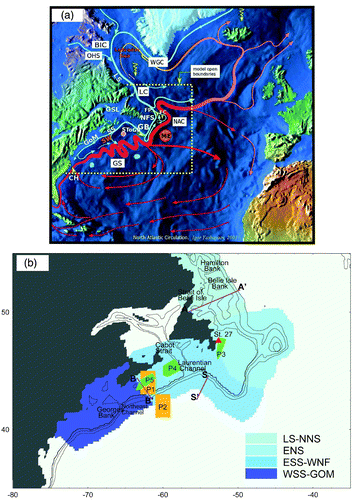
The eastern Canadian shelf (ECS) comprises the coastal and continental shelf waters from the Labrador Sea in the north to the Gulf of Maine in the south (Fig. 1). Dynamically this region lies in the western boundary confluence zone of two large-scale gyre systems: the North Atlantic subpolar gyre and the North Atlantic subtropical gyre (Loder et al., 1998). The coastal and shelf circulation on the ECS is predominantly influenced by the North Atlantic subpolar gyre and its western boundary current that flows equatorward: the Labrador Current. The ECS and adjacent waters are also affected by the Gulf Stream and its northern extension, the North Atlantic Current, both of which are western boundary currents of the North Atlantic subtropical gyre and lie offshore of the ECS (Fig. 1a). Previous studies have demonstrated that the ECS is the most variable area of the North Atlantic and Pacific oceans (Thompson et al., 1988), with the largest seasonal variations in water temperature, about 16°C, occurring over the Scotian Shelf and the Middle Atlantic Bight. Significant efforts have been made in the past to determine the general circulation, hydrographic distributions and associated seasonal variability of the ECS (Smith and Schwing, 1991; Lynch et al., 1996; Sheng and Thompson, 1996; Colbourne et al., 1997; Loder et al., 1998; Xue et al., 2000; Sheng et al., 2001; Han and Loder, 2003; Han et al., 2008). Efforts have also been made to examine the interannual variability over this region (Thompson et al., 1988; Petrie et al., 1992; Petrie and Drinkwater, 1993; Han and Tang, 2001; Han, 2007). Many questions, however, remain unanswered regarding the general circulation and associated temporal and spatial variability over the region. For example, what are the variations in the strength and equatorward extension of the Labrador Current beyond the Tail of the Grand Banks? How is the circulation over the ECS affected by the Gulf Stream and the North Atlantic Current? What are the main physical processes affecting the interannual variability of circulation and hydrography over the ECS? In this study, some of these issues are addressed using model results produced by a regional-scale coupled ocean–ice model.

Fig. 1 (a) Schematic of general upper-ocean circulation over the northwest Atlantic Ocean and the model domain marked by dashed lines (modified from the image created by Igor Yashayaev, reproduced by permission). (b) Topographic features over the eastern Canadian continental shelf. Model results over subregions with different colours are discussed in the paper. Model results over areas marked by P1 and P5 and indicated sections are used for the model validation and the process study of interannual variability. Abbreviations are used for the Gulf Stream (GS), North Atlantic Current (NAC), Labrador Current (LC), Mann Eddy (ME), West Greenland Current (WGC), Baffin Island Current (BIC), Outflow from Hudson Strait (OHS), Labrador Shelf (LS), Newfoundland Shelf (NFS), Scotian Shelf (SS), Gulf of Maine (GOM), Gulf of St. Lawrence (GSL), Slope Water (SW), Grand Banks (GB), Flemish Cap (FC), Flemish Pass (FP), Tail of the Grand Banks (SToGB), Cape Hatteras (CH).

This paper is structured as follows. Section 2 reviews the general mean circulation and observational evidence of interannual variability over the ECS. Section 3 summarizes the coupled ocean–ice model and external forcing. The assessment of the model performance is presented in Section 4, and the main mechanisms affecting the interannual variability over the ECS are discussed in Section 5. A summary and conclusions are given in Section 6.

2 Review of circulation and hydrographic features on the Eastern Canadian Shelf

The three-dimensional (3-D) circulation and hydrographic distributions over the ECS are affected by the topography of the region, which is highly irregular, with the coastline interrupted by several large gulfs, embayments, submarine banks and basins (Smith and Schwing, 1991; Loder et al., 1998). The Labrador Shelf is relatively straight and rugged and extends from Hudson Strait to the Strait of Belle Isle. The Newfoundland Shelf is situated along the coast of Newfoundland from Belle Isle Bank to Cabot Strait and Laurentian Channel, including the Grand Banks and Flemish Cap. The Gulf of St. Lawrence is a semi-enclosed sea connected to the North Atlantic Ocean through Cabot Strait and to the Labrador and Newfoundland shelves through the Strait of Belle Isle. To the west of Laurentian Channel lies the Scotian Shelf, which is connected to the Gulf of St. Lawrence to the northeast and to the Gulf of Maine to the southwest. The Gulf of Maine is also a semi-enclosed sea bounded by Georges Bank, Nantucket Shoals and Browns Bank at its seaward end and connects with the adjacent waters primarily through three main channels (Lynch et al., 1996).

a Mean Circulation over the Eastern Canadian Shelf

The general mean circulation over the ECS has been the subject of many field and modelling studies in the past. A comprehensive review of the mean circulation over the region can be found elsewhere (Smith and Schwing, 1991; Loder et al., 1998). The combination of the West Greenland Current, the Baffin Island Current and the outflow from Hudson Strait forms the “traditional” Labrador Current over the northern Labrador Shelf (Fig. 1a). At the Hamilton Bank section of the southern Labrador Shelf the Labrador Current has three branches: an inshore branch near the coast; an offshore branch over the shelf break; and a deep branch beyond the shelf break (Thompson et al., 1986; Lazier and Wright, 1993; Loder et al., 1998; Han et al., 2008). A small fraction of the inner branch of the Labrador Current enters the Gulf of St. Lawrence through the Strait of Belle Isle. The rest of the inner branch and the other two branches flow onto the Newfoundland Shelf. Over the northern Newfoundland Shelf, the Labrador Current has a coastal branch flowing through Avalon Channel to the coastal waters of southern Newfoundland, a middle branch following the shelf break through Flemish Pass, and an eastern branch passing around the seaward flank of Flemish Cap (Petrie and Anderson, 1983; Sheng and Thompson, 1996; Colbourne et al., 1997; Loder et al., 1998; Han et al., 2008). Part of the eastern branch of the Labrador Current over the northern Newfoundland Shelf moves into the deep ocean to join the North Atlantic Current, and the rest joins the middle branch to the south of the Flemish Pass (Han et al., 2008). Upon reaching the Tail of the Grand Banks, some of the Labrador Current turns offshore into the Newfoundland Basin, and the rest flows around the Tail and continues to flow equatorward along the shelf break of the southwestern Grand Banks.

Part of the Labrador Current that flows around the Tail of the Grand Banks reaches the eastern Scotian Shelf by crossing the Laurentian Channel (Han and Loder, 2003). The low-salinity water over the western Gulf of St. Lawrence emanates from the Gulf through the western side of Cabot Strait and moves onto the eastern Scotian Shelf where it mixes with the more saline slope water flowing onto the shelf and moves southwestward as the Nova Scotian Current (Hachey et al., 1954; Han and Loder, 2003). Over the western Scotian Shelf, the low-salinity Nova Scotian Current enters the Gulf of Maine at Cape Sable. In the deeper waters south of the Scotian Shelf break, Slope Water is found which has two distinct zones in the vertical: the near-surface Warm Slope Water and the sub-surface Labrador Slope Water. The former is a mixture of coastal water and Gulf Stream water that flows primarily eastward, while the latter is a mixture of Labrador Current and North Atlantic Central waters that flows mostly southwestward (McLellan, 1957; Gatien, 1976). The offshore branch of the Labrador Current reduces its transport while flowing along the Nova Scotia shelf break and entering the Gulf of Maine through the Northeast Channel (Hannah et al., 2001; Han, 2007).

b Interannual Variability in Circulation and Hydrography

Circulation and hydrography over the ECS exhibit large interannual variability (Weare, 1977; Petrie et al., 1992; Petrie and Drinkwater, 1993; Colbourne et al., 1997), which could have a significant impact on ecosystem dynamics in the region. There was a massive mortality of “warm-water” tilefish, for example, occurring between April and August of 1882 over the Middle Atlantic Bight. Marsh et al. (1999) attributed this massive tilefish kill to a sudden cooling in the region as a consequence of an enhanced equatorward transport of cold water in the Labrador Current. Based on in situ hydrographic observations, Petrie and Drinkwater (1993) showed that a cooling trend occurred on the Scotian Shelf and in the Gulf of Maine from 1952 to 1967, followed by a rapid warming trend from 1968 to 1978 and then by a slow decline from the late 1970s to 1990 (Figs 2a and 2b). They also revealed that the observed cooling (warming) trends on the Scotian Shelf and in the Gulf of Maine were correlated with freshening (increasing) salinity trends (not shown). The interannual variability of hydrography on the Scotian Shelf and in the Gulf of Maine was found to occur over the entire water column but with the largest amplitudes occurring in the subsurface waters. Petrie and Drinkwater (1993) suggested that the variability of the westward transport of the Labrador Current was responsible for the interannual variability of the water properties from the Gulf of St. Lawrence to the Gulf of Maine.

Fig. 2 Time series of monthly temperature anomalies (annual cycle removed) from 1945 to 1992 at (a) Georges Basin at 100 m, (b) the Slope Water region at 100 m. Depth-mean monthly (dashed) and five-year running average (solid) anomalies of temperature at (c) Flemish Cap and (d) Station 27 (modified from Petrie and Drinkwater (1993) by permission of the American Geophysical Union and Colbourne and Foote (2000) by permission of the Northwest Atlantic Fisheries Organization).

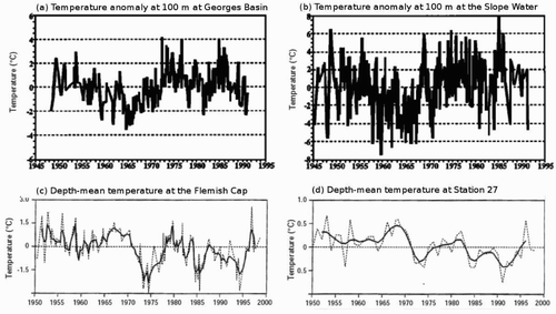
It was found that water masses over the Newfoundland Shelf have cooling and warming trends significantly different from the observed trends over the Scotian Shelf and the Gulf of Maine. Based on hydrographic observations at Station 27 (Fig. 1b) in the Avalon Channel over the inner Newfoundland Shelf, Petrie et al. (1992) discovered that a warming period in the late 1960s was followed by a cooling period in the early 1970s and then a warming trend into the early 1980s for water masses at Station 27. Figures 2c and 2d show the monthly anomalies and five-year running mean anomalies of temperature after removing the annual cycle at Flemish Cap and Station 27, respectively, indicating that a warming period occurred from the mid-1950s to the mid-1960s and significant cooling took place in 1966–71, 1982–84 and 1987–92. The period with the most significant cooling events over the Newfoundland Shelf was 1966–71 which corresponds to the period of the “Great Salinity Anomaly” in the subpolar gyre (Dickson et al., 1988). Petrie et al. (1992) and Colbourne and Foote (2000) suggested that the advection of Labrador Current water onto the Newfoundland Shelf was the main cause of the interannual variability observed over the region. Petrie et al. (1992) also suggested that the large regional differences in the surface ice extent and advection over the Labrador and Newfoundland shelves could explain why the interannual variability in sea surface temperature (SST) over these two shelves is virtually uncorrelated.

Satellite-derived SST observations over the central Scotian Shelf and Slope areas (P1 and P2 marked in Fig. 1b) revealed that the SSTs had significant interannual variability with a cooling trend in 1999–2004 (Shadwick et al., 2010). The cooling during this period is of the order of 2°C over the central Scotian Shelf and slightly less in the Slope Water region. There was a sharp temperature decline of about 4°C in the winter of 2003 over the Slope Water region. A similar, but smaller, decline also occurred over the central Scotian Shelf.

The occurrence of the interannual temperature variability is by no means restricted only to the sea surface of the ECS. Head and Sameoto (2007) demonstrated that the interannual variability also occurred in the depth-averaged temperature and salinity observations over the Newfoundland Shelf and the eastern and western Scotian Shelf. They showed that the depth-averaged temperatures over the western Scotian Shelf had marked cooling trends in 1995–98 and 2000–03 with a sharp warming tendency between these two periods. There was a significant warming period in 1997–2000 over the eastern Scotian Shelf that preceded a cooling trend in 2000–03. The cooling trend of the depth-averaged temperature from 2000–03 over the Scotian Shelf is correlated with the sea surface cooling reported by Shadwick et al. (2010). Based on a correlation analysis of the annual anomalies of the depth-mean temperature observations with the North Atlantic Oscillation (NAO) index, Head and Sameoto (2007) revealed that a positive (negative) NAO index tends to lead to reduced (increased) temperatures on the Newfoundland Shelf and to increased (reduced) temperatures on the central and western areas of the Scotian Shelf. In this study, the issue of determining the main physical processes affecting the interannual variability of circulation and hydrography over the ECS is addressed using model results produced by a regional-scale coupled ocean–ice model.

3 Coupled ocean–ice model

a Model Setup and Forcing

The numerical model used in this study is based on version 2.3 of the Nucleus for European Modelling of the Ocean (NEMO) modelling system (Madec, 2008), which uses version 9 of the Océan PArallélisé System (NEMO-OPA9) as the ocean circulation component and version 2 of the Louvain-la-Neuve Ice Model (NEMO-LIM2) as the sea-ice component. NEMO-OPA9 is a primitive-equation, finite difference ocean circulation model with a free sea surface and z-coordinate in the vertical (Madec, 2008). NEMO-LIM2 is a two-category (ice and open water) dynamic-thermodynamic sea-ice model (Timmermann et al., 2005).

The model domain covers the northwest Atlantic Ocean between 33°N and 55°N and between 80°W and 33°W (Fig. 1). The coupled ocean–ice model uses a horizontal curvilinear grid with a horizontal resolution of approximately 1/4° in longitude and approximately 1/4°cosϕ in latitude (ϕ). There are 46 z-levels in the vertical, with the vertical grid spacing increasing from 6 m in the uppermost z-level to 250 m at the lowermost z-level. The model bathymetry is taken from Earth Topography 2-arc-min (ETOPO2; Smith and Sandwell, 1997). The subgrid-scale horizontal mixing for momentum and tracers is parameterized using a biharmonic friction with a Smagorinsky-like mixing coefficient which varies horizontally as a function of the grid size and is also flow dependent (Griffies and Hallberg, 2000). The vertical subgrid-scale mixing is parameterized using the turbulent closure scheme of Gaspar et al. (1990). The model time step is 2400 s. The coupled ocean–ice model is initialized from the climatological monthly mean hydrography of Geshelin et al. (1999). The model is spun up from a state of rest and integrated for 18 years from the beginning of 1987 to 2004. Only the model results for the last 17 years are used in this study.

The atmospheric forcing used to drive the coupled ocean–ice model is taken from the reanalysis fields, with a horizontal resolution of 2° in both longitude and latitude, produced by Large and Yeager (2004). The atmospheric reanalysis data used in this study include 6-hourly fields of zonal and meridional wind speeds, specific humidity and air temperature at 10 m above the sea surface; 12-hourly fields of short- and longwave radiation; and monthly mean precipitation. All the atmospheric forcing fields are interpolated onto the model grid in time and space to obtain the momentum, heat and freshwater fluxes at the air–sea interface. The wind stress vector (τ) at the model sea surface is given by

where f_i is the fraction of the ocean surface covered by the sea ice, which is 1 if the ocean surface is fully covered by sea ice and 0 if there is no ice; τ _io is the ice-ocean momentum flux; and τ _ao is the air–ocean momentum flux without sea ice calculated from Large-Yeager's reanalyzed wind speeds using the formulation of Large and Pond (1981) with the transfer coefficient suggested by Large and Yeager, (2004).

The net heat flux (Q) at the sea surface is computed based on (Gill, 1982):

where Q_io represents the ice-ocean heat flux; Q_sw represents the incoming shortwave radiation into the ocean; Q_lw is the net longwave flux from the atmosphere to the ocean; Q_s is the sensible heat flux due to conduction; and Q_l is the latent heat flux carried by the evaporated water. The net heat fluxes are defined to be positive when heat is being transferred from the atmosphere into the ocean. The formulation of Large and Yeager (2004) is used to calculate the sensible and latent heat fluxes Q_s and Q_l .

The net freshwater flux (F) at the sea surface is computed based on (Large and Yeager, 2004):

where F_io is the freshwater flux between ice and water; E is the evaporative component of the freshwater flux; P is the precipitation over the ocean; and F_r is a term that restores the model sea surface salinity (S_m ) to the climatological monthly mean sea surface salinity (S_c ) defined as , where γ _s is a restoring time scale to reduce model drift and is set to two months. In addition, freshwater runoff from major rivers in the region is specified to a monthly climatology compiled by Barnier et al. (2006).

The lateral boundary conditions specified in the model are as follows. At the model closed boundaries, a free slip condition is applied, with zero normal fluxes of momentum, temperature and salinity. At three lateral (northern, eastern and southern) open boundaries, the normal flow, temperature and salinity fields are adjusted based on the adaptive open boundary condition (e.g., Stevens, 1990; Marchesiello et al., 2001; Sheng and Tang, 2003). An explicit Orlanski radiation condition is first used to determine whether the open boundary is passive (outward propagation) or active (inward propagation). If the open boundary is passive, the model prognostic variables (i.e., model currents, temperature and salinity) are radiated outward to allow perturbations generated inside the model domain to propagate outward as freely as possible. If the open boundary is active, the model prognostic variables at each z level are restored to the five-day time-mean currents, temperature and salinity extracted from the global ocean reanalysis data produced by Smith et al. (2010). A restoring time scale of 60 days is used for baroclinic currents, temperature and salinity at the three lateral open boundaries. An additional adjustment is made by restoring the depth-mean currents through the model open boundaries to the ocean reanalysis data with a restoring time scale of five days for the eastern and southern open boundaries and 40 minutes for the northern open boundary. The main reason for using a shorter restoring time scale at the northern open boundary is that this is the upstream border for shelf waves over the ECS. As a result, the northern open boundary condition significantly affects the circulation, hydrography and associated variability in the model domain, particularly over the Labrador and northern Newfoundland shelves (for further discussion see Section 5). In particular, we found that a longer restoring time scale would result in a subpolar gyre in the model that is too strong and would dominate the flow over the subtropical gyre.

b The Spectral Nudging Method and Semiprognostic Method

To reduce seasonal bias and drift in the model, a combination of the spectral nudging method (Thompson et al., 2006) and the smoothed semiprognostic method (Sheng et al., 2001; Greatbatch et al., 2004) is used. The spectral nudging method restores the model temperature and salinity in frequency-wavenumber bands that cover only information resolved by the hydrographic climatology (Thompson et al., 2007). In this study the spectral nudging method is used to restore the annual mean and the annual and semi-annual cycles of model temperature and salinity to the cycles determined from the monthly mean climatology produced by Geshelin et al. (1999). Outside these bands, the model temperature and salinity are not affected by the nudging and evolve prognostically. There are two key parameters in the application of this method: κ and γ. The first parameter (κ) specifies the band-pass width around the nudging frequencies where the nudging takes effect, and the second parameter (γ) determines the strength of the nudging such that large γ values imply weak nudging and vice versa. In this study κ is set to 3 years, which is similar to the values used previously; the value of γ is set to 200 days, which is a longer restoring time scale than the values used in other studies (Thompson et al., 2006, 2007; Wright et al., 2006).

Different from the spectral nudging method, the smoothed semiprognostic method adds a correction to the horizontal pressure gradient terms in the model momentum equation based on the smoothed differences between observed (ρ _c ) and modelled density (ρ _m ). The correction is made through the hydrostatic equation:

where p is the pressure; z is the vertical coordinate, positive upward; g is the accleration due to gravity; β is a coefficient ranging between 0 and 1; and the overbar represents a horizontal filter operator to eliminate small-scale features in the density difference term in the above equation. As a result, the smoothed semiprognostic method applies only to large-scale features. If β = 0, the model is purely prognostic, and if β = 1, the model is diagnostic in large-scale circulation features. This study uses a simple moving average with five points in the eastward and northward directions with β = 0.25, which is smaller than the typical value of 0.5 used in previous studies (Sheng et al., 2001; Eden et al., 2004; Zhao et al., 2006).

Both the spectral nudging and smoothed semiprognostic methods can be considered simple data assimilation techniques. The main purpose of any data assimilation is to improve model skill by modifying model dynamics by assimilating observations into the model. Based on the model sensitivity study, we found that the combination of the spectral nudging method and the smoothed semiprognostic method with coefficients that are smaller than usual for both methods is efficient in eliminating the seasonal model drift, while making the model more prognostic.

4 Model validation

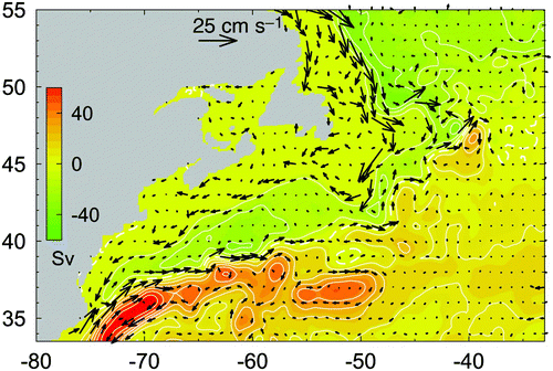
The performance of the NEMO coupled ocean–ice model in simulating the general circulation and interannual variability over the study region is assessed by comparing model results with previous observational and model results in the literature. Figure 3 presents the time-mean streamfunction of the depth-integrated flow simulated by the model over the 17-year period from 1988 to 2004. In comparison with previous numerical results published in the literature (e.g., Smith et al., 2000; Sheng et al., 2001; Wright et al., 2006; Han et al., 2008), the regional ocean circulation model reproduces the time-mean transports of the Labrador Current, the Gulf Stream, and the Northern Recirculation gyre over the slope water between the Scotian shelf and the Gulf Stream in the northwest Atlantic Ocean reasonably well. The maximum mean transport produced by the model is about 30 Sv (where 1 Sv = 10⁶ kg s⁻¹) for the Labrador Current, 80 Sv for the Gulf Stream and about 20 to 30 Sv for the recirculation over the slope water region, which are in good agreement with the results using different ocean circulation models but with similar horizontal resolutions (Sheng et al., 2001; Wright et al., 2006). The model also reproduces reasonably well the depth-integrated flow near the separation of the Gulf Stream at Cape Hatteras and the pathway of the Gulf Stream roughly from 75°W, 35°N to 50°W, 41°N to the south of the Grand Banks of Newfoundland.

Fig. 3 Time-mean streamfunction of the depth-integrated flow calculated from model currents in the 17-year period 1988–2004 with the arrows indicating the depth-averaged currents over the model domain. The contour interval is 10 Sv and the dashed line represents the 0 Sv contour.

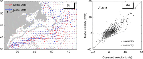
Higginson et al. (2011) recently produced a time-mean sea surface topography (MSST) of the northwest Atlantic to study the mean circulation of the subpolar gyre from nine years of altimetry observations referenced with respect to a new regional geoid based on a blend of the Gravity Recovery and Climate Experiment (GRACE), terrestrial, and altimetry-derived gravity data. From a subset of the altimetry-derived MSST, the time-mean surface geostrophic currents were calculated based on the geostrophic balance (Higginson et al., 2011). Similarly, the time-mean model surface geostrophic currents can be calculated from the time-mean model sea surface elevations. Figure 4a presents the comparison of the model-calculated and altimetry-derived surface geostrophic currents. The circulation model reproduces the altimetry-derived surface geostrophic currents very well, particularly the intense surface geostrophic currents associated with the Gulf Stream after its separation point at Cape Hatteras. The circulation model also performs reasonably well in simulating the strong poleward geostrophic currents associated with the North Atlantic Current in the deep waters to the east of the Grand Banks and over the northeast corner as well as the equatorward geostrophic currents associated with the inshore and offshore branches of the Labrador Current over the Labrador Shelf. There are large differences between the simulated and altimetry-based surface geostrophic currents over the coastal and shelf waters of the ECS which might be attributed to some extent to errors associated with satellite altimeter measurements near the coast. The regional model also performs less well in simulating the anticyclonic circulation and the Mann Eddy to the east of the Grand Banks (Fig. 4a).

Fig. 4 (a) Comparison of time-mean surface geostrophic currents in the five-year period 2000–04 calculated from the simulated (blue) and altimetry-derived (red) time-mean sea surface elevations (data from Higginson et al. (2011)). (b) Scatterplot of altimetry-derived and simulated time-mean surface geostrophic currents.

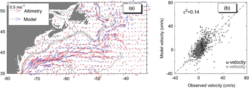
Figure 4b shows the scatterplot of eastward and northward components of altimetry-derived and simulated surface geostrophic currents. To quantify the fit between the altimetry-derived and simulated currents shown in Fig. 4a, the ε² value defined as follows is used:

where (, ) and (, ) represent, respectively, the eastward and northward components of the altimetry-derived and simulated surface geostrophic currents at the ith location of altimetry-derived currents, and N is the total number of locations. The ε² value ranges between 0 and 1. The model currents agree perfectly with the observations if ε² = 0, and the model does not have any skill if ε² = 1. The value of ε² is 0.14 for the results in Fig. 4b, indicating that the regional model has good skill in simulating the time-mean surface geostrophic circulation derived from altimetry data.

The ocean circulation, particularly in the upper ocean, has strong ageostrophic currents (such as wind-driven currents, see Fig. 1a in Trossman et al. (2009)), in addition to the geostrophic currents discussed above. To assess the model performance in simulating the general circulation over the ECS, the time-mean sub-surface (15 m) currents derived from satellite-tracked drifting buoys drogued at 15 m depth between 1980 and 2005 (Niiler, 2001) are compared to the time-mean sub-surface currents calculated from model currents at 15 m in the period between 1988 and 2004. Figure 5a demonstrates that the model reproduces well the drifter-derived time-mean sub-surface currents associated with the Gulf Stream and the North Atlantic Current in the deep waters off the ECS. Over the Labrador Shelf, the model generates relatively strong inshore and offshore branches of the Labrador Current with maximum speeds of about 20 and 30 cm s⁻¹, respectively. The model also simulates well the bifurcation of the inshore Labrador Current before reaching Belle Isle Bank, with one branch flowing into the Gulf of St. Lawrence through the Strait of Belle Isle and the other branch flowing southward to the inshore waters of the Newfoundland Shelf. Over Flemish Pass and Flemish Cap and the eastern flank of the Grand Banks, the simulated time-mean sub-surface currents have the typical circulation features discussed in Section 2, featuring a southeastward throughflow over Flemish Pass, an anticyclonic gyre over Flemish Cap and an intense southwestward flow over the eastern flank of the Grand Banks. Figure 5b shows the scatterplot of eastward and northward components of drifter-derived and simulated time-mean sub-surface currents at 15 m depth. By using Eq. (5) with (, ) and (, ) as the eastward and northward components of the drifter-derived and simulated time-mean sub-surface (15 m) currents, respectively, we obtain a value of ε² of approximately 0.11. This indicates again that the model has very good skill in simulating the time-mean sub-surface (15 m) circulation derived from the trajectories of drifters.

Fig. 5 (a) Comparison of time-mean currents at 15 m inferred from sub-surface drifter movements (data from Niiler (2001)) and computed from 3-D model results (blue) and (b) scatterplot of drifter-derived and simulated time-mean horizontal currents over the northwest Atlantic.

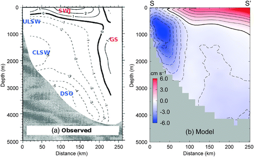
Based on the measurements made with Conductivity-Temperature-Depth (CTD) sensors and acoustic transport floats as well as measured dissolved oxygen and chlorofluorocarbons along a transect across the southwestern Newfoundland Slope (S–S′ in Fig. 1b) between 1983 and 1995, Pickart and Smethie (1998) calculated the time-mean absolute geostrophic velocity normal to the transect (Fig. 6a). The vertical structure of the horizontal flow across the transect features equatorward currents associated with the upper Labrador Sea Water (ULSW; centred at about 800 m) originating from the western Labrador Sea, the classical Labrador Sea Water (CLSW; at about 1500 m) originating from the central Labrador Sea, and the Denmark Strait Overflow (DSO; at about 3500 m). Figure 6 also shows the poleward Slope Water Jet (SWJ) across the transect separating the Gulf Stream from the shelf break and from Labrador Sea Water in the top 500 m (Pickart and Smethie, 1998). The SWJ flows in the upper ocean with an eastward velocity of the order of 3 cm s⁻¹ and extends to a depth of about 300 m in the northern side and from the surface to about 500 m in its offshore side (Fuglister and Worthington, 1951). Figure 6b presents the vertical distribution of time-mean horizontal currents normal to the same transect between 1988 and 2004 averaged from model results. The regional circulation model reproduces both the eastward SWJ and the westward Labrador Current in the upper and intermediate continental slope reasonably well, with simulated currents relatively stronger than the observations discussed by Pickart and Smethie (1998). It should be noted that the simulated Denmark Strait Overflow (DSO) is relatively weaker, and its position is further offshore than the observations (Fig. 6). A possible explanation for this discrepancy is that the circulation shown in Fig. 6a uses time-averaged observations collected over only three periods (in 1991, 1994, 1995) each of which spanned about one week. Therefore, caution should be taken in considering the pattern shown in Fig. 6a to be the true representation of the time-mean flow.

Fig. 6 (a) Absolute geostrophic currents estimated from time-mean hydrographic observations at a transect off the southwestern Newfoundland Shelf at approximately 55°W (reprinted from Pickart and Smethie (1998) by permission of Elsevier). (b) Time-mean currents normal to the transect computed from model results between 1988 and 2004. Black contour lines indicate velocity contours spaced every 1 cm s⁻¹ with the thick black line indicating the zero velocity contour. Abbreviations are used for the Slope Water Jet (SWJ), Upper Labrador Sea Water (ULSW), Classical Labrador Sea Water (CLSW), Denmark Strait Overflow (DSO) and the Gulf Stream (GS).

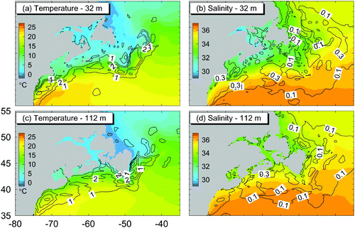
We next examine the model performance in simulating the seasonal cycle of hydrography over the study region. Figure 7 presents the 17-year time-mean temperature and salinity at depths of 32 and 112 m calculated from 3-D model results between 1988 and 2004. The regional circulation model reproduces the general distributions of temperature and salinity over the northwest Atlantic. The model also reproduces relatively cold and fresh waters carried by the Labrador Current from the Labrador Shelf to the Tail of the Grand Banks and then to the shelf break of the Scotian Shelf and warm and salty waters carried by the Gulf Stream and the North Atlantic Current from the tropical waters to the deep waters off the ECS. The model successfully simulates the relatively cold and fresh waters in the western Gulf of St. Lawrence, over the inner Scotian Shelf and inner Gulf of Maine, which are primarily driven by the equatorward coastal currents associated with freshwater discharge from the St. Lawrence River.

Fig. 7 Colour images showing time-mean temperature (a and c) and salinity (b and d) at depths of 32 and 112 m calculated from 3-D model results between 1988 and 2004. The black contours are the mean absolute differences between the climatological and simulated monthly mean temperature and salinity at the two depths.

To quantify the model skill in simulating the seasonal cycle of 3-D hydrography over the ECS, we calculated the average absolute difference (AAD) between the climatological and simulated monthly mean hydrography at each model grid point defined as

where and are the climatological and simulated monthly mean temperatures (or salinity), respectively. The climatological monthly mean values are taken from the 3-D gridded fields constructed by Geshelin et al. (1999). The simulated time-mean monthly mean values are calculated from model results between 1988 and 2004. The AADs are relatively small over the northwest Atlantic, except for the continental slope region and adjacent waters of the ECS (Fig. 7), indicating the efficiency of the spectral nudging method and the smoothed semiprognostic method in suppressing the seasonal bias and drift in the model. The AAD values for temperature at 32 m and 112 m are less than 1°C over coastal and shelf waters of the ECS but are relatively large over the continental slope region and also the area to the north of Cape Hatteras near the separation point of the Gulf Stream. The AAD values for salinity at these two depths are less than 0.1 (practical salinity scale used) in the deep ocean but slightly higher over the continental slope and shelf regions of the ECS with the largest AAD being about 0.3. The AAD values for salinity are similar in magnitude in the upper and sub-surface waters of the northwest Atlantic, except for the area to the north of the separation point of the Gulf Stream, where the AAD values are larger in the upper ocean. It should be noted that a simple optimal interpolation scheme was used in constructing the monthly mean climatology of hydrography from sparse hydrographic observations (Geshelin et al., 1999). Therefore, large AAD values over the continental slope region of the ECS are partially associated with relatively larger errors in the gridded monthly mean climatology over the slope region than in other regions.

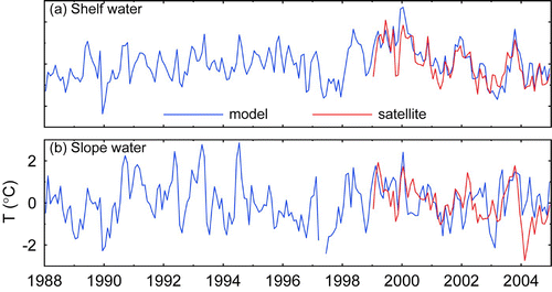
To demonstrate the model performance in simulating interannual variability of hydrography over the ECS, the monthly mean SST anomalies calculated from the model results are compared with the SST anomalies estimated from the satellite remote sensing data (Shadwick et al., 2010) between 1999 and 2005 over the Scotian Shelf and Slope (Fig. 8). The cooling trend from 1999 to 2005 at the ocean surface as seen from satellite observations is well reproduced by the model over the Scotian Shelf (Fig. 8a) and associated Slope region (Fig. 8b). It should be noted that the cooling trend during this period is actually part of the interannual variations in the SST as shown in the model results. Figure 8 also demonstrates that the model simulates the SST over the shelf waters better than over the slope waters because of complicated dynamics over the latter region (further discussion is provided in Section 5).

Fig. 8 Monthly mean anomalies of sea surface temperature derived from satellite remote sensing data (Shadwick et al., 2010) and calculated from model results for (a) an area over the central Scotian Shelf centred at 44°N and 64°W (P1 in Fig. 1) and (b) an area over the Slope Water region centred at 42°N and 60°W (P2 in Fig. 1).

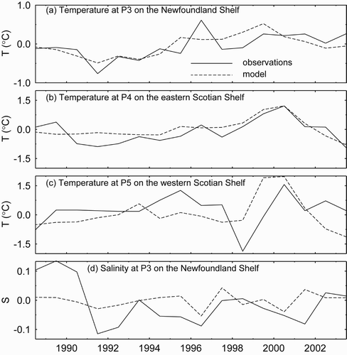
Figure 9 presents the annual-mean and depth-averaged observed anomalies of temperature and salinity over the Newfoundland and Scotian shelves (Head and Sameoto, 2007) compared with the depth-averaged annual mean simulated anomalies calculated from the 3-D model results for the period 1988–2004. The observed temperature anomalies over the Newfoundland and Scotian shelves are reasonably well reproduced by the model. In comparison, the observed annual mean salinity anomalies at P3 on the Newfoundland Shelf are less well reproduced by the model. We speculate that less realistic specification of the freshwater flux at the sea surface and unsolved processes for the sea-ice dynamics in the model are responsible for the model deficiency in simulating the observed salinity anomalies over the Newfoundland Shelf.

Fig. 9 Comparison of annual mean anomalies of observed hydrography over the Newfoundland and Scotian shelves (data from Head and Sameoto (2007)) with annual mean anomalies from model results for (a) temperature at P3 over the Newfoundland Shelf; (b) temperature at P4 over the eastern Scotian Shelf; (c) temperature at P5 over the central and western Scotian Shelf and (d) salinity at P3 at the Newfoundland Shelf.

5 Interannual variability over the eastern Canadian shelf

a Numerical Experiments with Different Model Forcing

There are three main mechanisms that affect the interannual variability of the circulation and hydrography in the model: (a) interannual variability in the atmospheric forcing, including surface wind stress and net sea surface heat and freshwater fluxes; (b) interannual variability in the flow and hydrography specified at the model open boundaries; and (c) model internal dynamics, mostly the model non-linear dynamics. Model results in four different numerical experiments are discussed in this section to examine the main physical processes affecting the interannual variability of circulation and hydrography over the ECS. The four experiments use the same NEMO coupled ocean–ice model with the same model setup, except for different model forcing as follows:

•	Exp-Control: The model in this experiment (control run) is driven by the suite of external forcing presented in Section 3. Some model results in this experiment were presented in Section 4.
•	Exp-ConstAll: The model in this experiment is driven by the time-mean atmospheric forcing taken from 18-year time-mean fields of surface winds, sea surface air temperature, specific humidity of the air, short- and longwave radiation, and precipitation calculated from Large-Yeager's atmospheric reanalysis data. The model is also driven by the time-mean boundary forcing at the three model open boundaries taken from the ocean reanalysis data produced by Smith et al. (2010). In this run, model interannual variability results from the non-linear (internal) dynamics in the model (assuming that long-term model drift is small).
•	Exp-ConstOBC: The model in this experiment is driven by the same external forcing as in Exp-Control, except for the 18-year time-mean boundary forcing at the three model open boundaries. Interannual variability in the experiment comes from the non-linear (internal) dynamics in the model as well as from the interannual variability in the atmospheric forcing fluxes.
•	Exp-ConstFluxes: The model in this experiment is driven by five-day mean temperature, salinity and currents at the lateral open boundaries taken from the global ocean reanalysis data, which are the same data used in Exp-Control. The model in this experiment is different from Exp-Control in that it is forced by the 18-year time-mean wind speed, air temperature, specific humidity of the air, short- and longwave radiation, and precipitation. Interannual variability produced by the model in the experiment comes from the non-linear (internal) dynamics in the model and the interannual variability through the model lateral open boundaries.

Except where otherwise stated, the monthly mean results of the 3-D model temperature, salinity and horizontal currents in the 17-year period 1988–2004 in each experiment were used for the analysis of interannual variability over the ECS in this section. We followed Petrie and Drinkwater (1993) and subtracted the 17-year monthly averages of currents and hydrography from the 3-D monthly mean model results at each model grid point to generate the monthly mean anomalies. Figure 10a presents the monthly mean anomalies of temperature and salinity in the control run (Exp-Control) averaged vertically between 100 and 300 m at seven locations along the shelf break of the ECS. It should be noted that the monthly mean anomalies of temperature and salinity at the northern open boundary (Figs 10a (inset a-0) and 10b (inset b-0)) were taken from the ocean reanalysis data of Smith et al. (2010).

Fig. 10 Monthly mean anomalies of sub-surface (100–300 m) model (a) temperature and (b) salinity at seven locations (marked by solid triangles) along the shelf break of the eastern Canadian Shelf in Exp-Control (solid) and Exp-ConstAll (dashed).

The monthly mean model temperature and salinity anomalies at intermediate depths of 100–300 m over the shelf break of the ECS in the control run have significant low-frequency (time scales longer than one year) variations, which are consistent with previous observations made in the region (Petrie et al., 1992; Petrie and Drinkwater, 1993; Colbourne and Foote, 2000). The maximum monthly mean anomalies of sub-surface (100–300 m) temperature and salinity in the control run are about 1°C and 0.2, respectively, over the shelf breaks of the Labrador and northern Newfoundland shelves; and about 2°C and 0.5, respectively, over the shelf breaks of the southwestern Newfoundland and Scotian shelves. Figure 10 also demonstrates that the sub-surface temperature and salinity anomalies at the shelf breaks of the Labrador and northern Newfoundland shelves are coherent with the anomalies at the northern open boundary, much more than the anomalies at the shelf breaks of the western Newfoundland and Scotian shelves.

Correlation analysis is used to calculate the correlation coefficients and time lags between the anomalies specified at the northern open boundary and the anomalies produced by the model in Exp-Control at different positions along the shelf break of the ECS shown in Fig. 10. The monthly mean anomalies of sub-surface hydrography at the shelf breaks of the ECS are correlated with the anomalies at the northern open boundary with correlation coefficients decreasing from a maximum of 0.9 over the Labrador Shelf to less than 0.4 over the eastern Scotian Shelf (Figs 11a and 11b). The time lags increase from about one month over the Labrador Shelf to about five months over the Scotian Shelf, indicating the equatorward propagation of the anomalies associated with the Labrador Current. It should be noted that the correlation between the sub-surface hydrographic anomalies at the shelf breaks of the central and western Scotian Shelf and the Gulf of Maine and the anomalies specified at the northern open boundary is small (less than 0.3), indicating that the interannual variability over these regions is significantly affected by physical processes other than the Labrador Current.

Fig. 11 Correlation coefficients between the monthly mean (a) temperature and (b) salinity anomalies at six different positions along the shelf breaks of the eastern Canadian shelf and the anomalies at the northern open boundary (OB); (c) and (d); as in (a) and (b) but for the correlation coefficients between the temperature and salinity anomalies with the winter North Atlantic Oscillation index (NAO). Different line colours represent the different locations shown in Fig. 10.

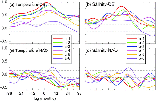
A similar correlation analysis was made for the temperature and salinity anomalies presented in Fig. 10 with the winter NAO index (Figs 11c and 11d). The correlations are about 0.4 and statistically significant over the Labrador Shelf and the eastern Newfoundland Shelf, indicating that cooler and fresher conditions lag (by about one year) positive NAO phases, which is consistent with the findings of Petrie (2007). Over the southern Newfoundland Shelf and the Scotian Shelf the correlations are smaller and often below the significance level.

The other important processes that could affect the interannual variability over the Slope Water off the Scotian Shelf include the interannual variability in the wind forcing and heat and freshwater fluxes at the sea surface and anomalies produced by the non-linear dynamics in the model. To identify which processes play a dominant role, the monthly mean anomalies of sub-surface temperature and salinity in the control run (Exp-Control) are compared with the Exp-ConstAll case (Fig. 10). In comparison with the model results in Exp-Control, the monthly mean anomalies of sub-surface temperatures and salinity in Exp-ConstAll are relatively small at the shelf breaks of the Labrador and northern Newfoundland shelves and have similar large variations but with different phases at the shelf break of the Scotian Shelf. Figure 10 also demonstrates that at the shelf breaks of the southern Newfoundland Shelf in the ConstAll case, the sub-surface temperature anomalies are relatively large and the sub-surface salinity anomalies are relatively small. It should be noted that the external model forcing in Exp-ConstAll does not have any interannual variability. As mentioned before, the monthly anomalies in model results in Exp-ConstAll are caused solely by the non-linear dynamics in the model.

b The Complex Empirical Orthogonal Function Analysis

The Complex Empirical Orthogonal Function (CEOF) analysis is used to identify the advective processes affecting the interannual variability over the ECS in the model. The CEOF analysis is a multivariate statistical technique for extracting the dominant spatial patterns of variability from data series (Horel, 1984; Terradas et al., 2004). In comparison with the conventional Empirical Orthogonal Function (EOF) method for determining statistically the spatial patterns coherent only at zero lag (Hannachi et al., 2007); the CEOF analysis has the advantage of isolating propagating and standing patterns. The first step in a CEOF analysis is to construct a complex field Ψ(x, t) from the scalar field of monthly mean temperature (or salinity) anomalies T(x, t):

where x represents the position vector, t is time, , and H(x, t) represents the Hilbert transformation of T(x, t). Hilbert transformation means that the amplitude of each Fourier spectral component of T(x, t) is unchanged while its phase is advanced by π/2 (Horel, 1984). Since Ψ is complex, the eigenfunctions E_n (x) and mode coefficients A_n (t) (with n = 1, 2, 3 … N) resulting from the EOF analysis of Ψ(x, t) are also complex. The complex field Ψ can be expressed in terms of E_n (x) and A_n (t):

where R_n (t) is the temporal amplitude function of A_n (t); ϕ _n (t) is the temporal phase function defined as ϕ _n (t) = arctan[Im(A_n )/Re(A_n )]; S_n (x) is the spatial amplitude function of E_n (x); and θ _n (x) is the spatial phase function defined as θ _n (x) = arctan[Im(E_n )/Re(E_n )]. Physically, the temporal amplitude function (R_n ) describes the temporal variability in the magnitude associated with the nth eigenfunction, and the temporal phase function (ϕi_n ) describes the temporal variation of the phase of the nth eigenfunction associated with periodicities in T(x,t). The spatial amplitude function (S_n ) describes the spatial distribution of variability associated with each eigenfunction, and the spatial phase function (θ _n ) describes the relative phase function among various spatial locations. For a standing wave pattern, S_n has the structure of nodes and antinodes, and θ _n has a jump of π between the two neighbouring antinodes. For propagating waves, the spatial phase function θ _n changes with space (Terradas et al., 2004). Furthermore, the time derivative of ϕ _n is a measure of the “instantaneous” frequency(dϕ _n/dt), while the spatial derivative of θ _n provides a measure of the “local” wavenumber calculated using ∂ θ _n  / ∂x, ∂ θ _n  / ∂y.

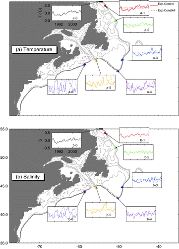
Because of large regional differences in circulation and interannual variability over the ECS (Petrie et al., 1992; Petrie and Drinkwater, 1993), the CEOF analysis is performed separately for the monthly mean anomalies of model temperatures and salinity over four subregions (Fig. 1b): (1) the Labrador Shelf, the northern Newfoundland Shelf and adjacent waters (LS-NNS); (2) the eastern Newfoundland Shelf and adjacent waters (ENFS); (3) the western Newfoundland Shelf, eastern Scotian Shelf and adjacent waters (WNFS-ESS); and (4) the western Scotian Shelf, Gulf of Maine and adjacent waters (WSS-GOM). In each subregion, the CEOF analysis is performed separately for the monthly mean anomalies of the 3-D temperature and salinity in three different vertical layers: (a) the upper layer 0–102 m, (b) an intermediate layer 102–350 m, and (c) a deep layer 350–1215 m. Because the model resolution used in this study is not spatially uniform, the monthly mean model temperature and salinity anomalies at each grid are weighted by the ratio of the grid volume to the maximum gridpoint volume over the subregion before performing the CEOF analysis. After the analysis, the spatial amplitude function S_n (x) is deweighted by the same ratio to ensure the resulting fields have meaningful units.

c Monthly Mean Anomalies over the Eastern Canadian Shelf

1 The Labrador and Northern Newfoundland Shelves

Table 1 lists percentages of the total variance explained by the first three CEOFs for the monthly mean temperature and salinity anomalies in three layers over this subregion in the control run. The first CEOF explains about 52%, 62% and 86% of the total variance in the temperature anomalies in the three layers, respectively. The second CEOF explains only about 14%, 11% and 7% of the total variance in the three layers, respectively. The third CEOF explains approximately 9% of the total variance in the three layers. For the monthly mean salinity anomalies in the three layers, the first three CEOFs also explain similar percentages of the total variance. This suggests that the first CEOF plays a very important role in the temperature and salinity anomalies over this subregion.

Table 1. Percentages of the total variance explained by the first three CEOFs extracted from the monthly mean temperature and salinity anomalies in the three layers over the Labrador Shelf and northern Newfoundland Shelf in the control run.

Layer	Percentage of variance
	Temperature			Salinity
	mode 1	mode 2	mode 3	mode 1	mode 2	mode 3
Upper	51.5	14.1	7.3	50.9	10.2	8.9
Intermediate	62.3	11.3	8.2	47.5	13.8	7.8
Lower	85.7	6.8	2.8	88.8	4.7	2.0

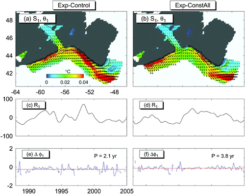
Figure 12 presents horizontal distributions of the spatial amplitude (S ₁) and phase vectors (θ₁) of the first CEOF, with the time series of the associated temporal amplitude (R ₁) and temporal phase change (Δϕ₁) for the monthly mean temperature anomalies at 160 m over the LS-NNS subregion in the control run. The spatial amplitude S ₁ over this subregion is nearly spatially uniform with relatively larger values over Hamilton Bank and at the shelf break than other areas (Fig. 12a). The clockwise rotation of the phase vectors from the northern to the southern part of the subregion indicates the direction of propagation of the patterns. The spatial phase vectors θ₁ have phase differences of less than 40 degrees over this subregion, indicating long wavelengths (and faster phase speeds) of the waves. Distributions of S ₁ and θ₁ shown in Fig. 12a indicate that the first CEOF in the control run represents the southeastward propagation of interannual variability of temperature anomalies from the Labrador Shelf to the northern Newfoundland Shelf with wavelengths of the order of 3000 km. The temporal amplitude R ₁ over this subregion (Fig. 12c) has significant low-frequency variations, with the time-mean period (P) of the variability being about 4.7 years (estimated from the time change of the temporal phase Δϕ in Fig. 12e, as P = 2πΔt/Δϕ, with Δt = 1/12 yr) which means phase speeds of the order of 2 cm s⁻¹.

Fig. 12 Distributions of spatial amplitude (S ₁) and phase (θ₁; arrows), temporal amplitude (R ₁) and temporal phase change (Δϕ₁) of the first CEOF for the monthly mean temperature anomalies at 160 m over the Labrador and northern Newfoundland shelves in Exp-Control (left panels) and Exp-ConstFluxes (right panels). The red line in the bottom panels represents the averaged temporal phase change.

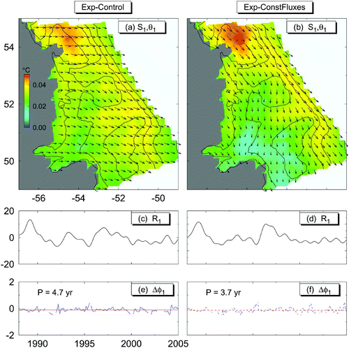
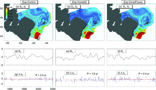
As shown in Fig. 10, the model temperature and salinity anomalies in Exp-ConstAll are small over the LS-NNS subregion, indicating that the non-linear dynamics play a minor role in the interannual variability over the LS-NNS subregion in the model. Therefore, only the anomalies in the sea surface forcing and boundary forcing in the model could be responsible for the CEOF shown in Fig. 12a. Figure 12 demonstrates that the spatial amplitude and phase functions of the first CEOFs in Exp-Control and Exp-ConstFluxes have very similar large-scale features, with similar temporal amplitude time series. The model external forcing, except for the model open boundary condition, is time-invariant in Exp-ConstFluxes, as mentioned earlier. This suggests that the interannual variability over this subregion in the control run is driven mostly by the variability at high latitudes that enter this subregion through the northern open boundary of the model.

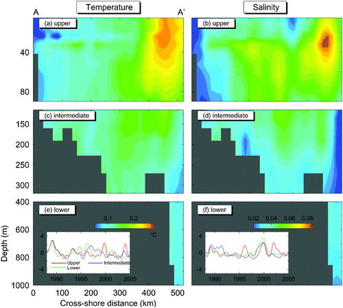
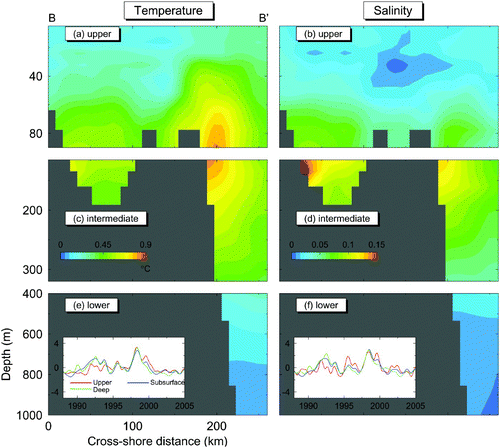
Figure 13 shows the vertical distribution of the spatial amplitude of the first CEOF (S ₁) for model temperature and salinity anomalies in the control run along transect AA′ at White Bay (Fig. 1b). The temporal amplitude R ₁ in each layer is normalized by its standard deviation and the spatial amplitude S ₁ is multiplied by its standard deviation in order to compare the vertical distributions of S ₁ in different layers. The spatial amplitude S ₁ has similar vertical distributions for temperature and salinity anomalies at transect AA′, featuring relatively larger values in the top 200 m and smaller values in the lower layer of the transect, with a maximum at about 40 m over the shelf break of the transect. Colbourne et al. (1997) revealed an intense southward jet in the top 100 m at Seal Island close to transect AA′. This suggests that the southward advection of the interannual variability carried by the offshore branch of the Labrador Current is responsible for the maximum interannual variability in the monthly mean temperature and salinity in the upper layer of the transect shown in Fig. 13.

Fig. 13 Vertical distributions of spatial amplitude functions (S ₁) of the first CEOF for the temperature (left panels) and salinity (right panels) anomalies in the upper (upper panels), intermediate (middle panels) and lower (lower panels) layers along section AA′ at White Bay on the northern Newfoundland Shelf.

2 The Eastern Newfoundland Shelf and Adjacent Waters

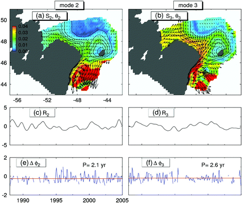
The CEOFs extracted from the monthly mean temperature and salinity anomalies over this subregion (ENFS) are significantly different from the CEOFs over the LS-NNS subregion. The first CEOF explains only about 27%, 31% and 44% of the total variance in the monthly mean salinity anomalies in the three vertical layers and percentages for the temperature anomalies over the ENFS subregion are similar (Table 2), which are about 1.5 to 2 times smaller than the percentages of the total variance explained by the first CEOF over the LS-NNS subregion. The spatial amplitude of the first CEOF over this subregion in the control run (S ₁) has large values in the deep waters to the east of the Grand Banks and relatively small values over other areas (Fig. 14a). For the deep water areas where the spatial amplitude is large, the spatial phase of the first mode (θ₁) in the control run features a clockwise rotation (of about 30°) of the phase vectors from south to north, indicating that the first CEOF in the control run shown in Fig. 14 represents poleward moving waves with wavelengths of the order of 3000 km and a time-mean period of about 3.3 years for the temperature anomalies and 2.4 years for the salinity anomalies. In the three cases of Exp-Control, Exp-ConstAll and Exp-ConstFluxes, the spatial amplitude functions (S ₁) have similar large-scale horizontal structures (Figs 14a–14c) and the temporal amplitude functions R ₁ have magnitudes of the same order (Figs 14d–14f), indicating that the large interannual variability in the deep waters to the east of the Grand Banks is mainly associated with the non-linear dynamics of the Labrador Current and the North Atlantic Current.

Table 2. Percentages of the total variance explained by the first three CEOFs extracted from the monthly mean temperature and salinity anomalies in the three layers over the eastern Newfoundland Shelf in the control run.

Layer	Percentage of variance
	Temperature			Salinity
	mode 1	mode 2	mode 3	mode 1	mode 2	mode 3
Upper	29.9	13.2	8.4	26.8	16.5	11.9
Intermediate	35.7	14.5	8.5	31.1	15.2	10.7
Lower	45.2	15.0	8.7	43.6	19.3	11.4

Fig. 14 Distributions of spatial amplitude (S ₁) and phase (θ₁; arrows), temporal amplitude (R ₁) and temporal phase change (Δϕ₁) functions of the first CEOF for the monthly mean salinity anomalies at 160 m over the eastern Newfoundland Shelf and adjacent waters in Exp-Control (left panels), Exp-ConstAll (centre panels) and Exp-ConstFluxes (right panels). The red line in the bottom panels represents the averaged temporal phase change.

The second and third CEOFs shown in Fig. 15 feature large spatial amplitudes in the deep waters to the east of the Grand Banks which are similar to the first CEOF, except that the second and third CEOFs have moderate amplitudes with moderate spatial phase differences along the shelf break from the Northern Newfoundland Shelf to the eastern Grand Banks through Flemish Pass. The second and third CEOFs represent equatorward propagating waves of interannual variability along the shelf break from the northern Newfoundland Shelf to the the eastern flank of the Grand Banks through Flemish Pass, in addition to the standing waves in the deep waters to the east of the Grand Banks.

Fig. 15 Distributions of spatial amplitude (S ₁) and phase (θ₁; arrows), functions of the second (left panels) and third (right panels) CEOFs for the monthly mean temperature anomalies at 160 m over the eastern Newfoundland Shelf and adjacent waters in the control run.

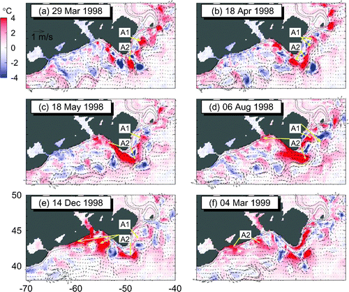
Figure 16 presents the time evolution of the anomalies of the sub-surface (160 m) temperatures and currents taken from five-day mean model results with seasonal cycles removed from the five-day model mean temperature and currents. (The seasonal cycles were interpolated linearly from the 17-year monthly-mean temperature and currents.) The anomalies shown in the figure have significant temporal and spatial variations. In the deep waters between the shelf break of the eastern Grand Banks and the western edge of the North Atlantic Current, there are many positive and negative temperature anomalies which move very slowly, either northward or southward, depending on the competing influences of the Labrador Current and the North Atlantic Current. We focus on the positive temperature anomaly labelled “A1” in Fig. 16 as an example. This temperature anomaly is centred at about 47°W and 45°N in late March 1998 (Fig. 16a). Anomaly A1 undergoes stretching and transforming at its original position in April and May (Figs 16b and 16c) and then separates into two parts in early August (Fig. 16d). The eastern part of anomaly A1 moves northward with the North Atlantic Current, and the western part is entrained by the Labrador Current and moves equatorward to the Tail of the Grand Banks and then to the southwestern flank of the Grand Banks in mid-December 1998 (Fig. 16f). During this period, a positive temperature anomaly labelled “A2” has very different movements. In late March 1998, anomaly A2 is centred at about 49°W and 41°N surrounded by three negative anomalies in the deep waters to the south of the Tail of the Grand Banks. Anomaly A2 undergoes significant stretching in April and May with its northwestern part advected equatorward by the Labrador Current along the shelf break of the southwestern Newfoundland Shelf (Figs 16b and 16c). The main part of anomaly A2 remains at its original position in early August and then moves westward onto the Slope Water region off the Scotian Shelf in December 1998 (Fig. 16e). It should be noted that as the northern part of anomaly A2 moves equatorward along the shelf break of the WNFS-ESS subregion, some of the northern parts enter the southern Gulf of St. Lawrence through Laurentian Channel (Fig. 16e). The northern part of anomaly A2 also affects the water properties in Emerald Basin by changing the monthly temperature fields from negative (Figs 16a–16d) to positive anomalies (Figs 16e–16f) once it reaches the central Scotian Shelf.

Fig. 16 Temperature anomalies at 160 m over the Scotian Shelf and Newfoundland Shelf region at six different times in 1998–99: (a) 29 March 1998; (b) 18 April 1998; (c) 18 May 1998; (d) 6 August 1998; (e) 14 December 1998; and (f) 4 March 1999. A long-term monthly mean cycle has been removed from the five-day anomalies.

3 The Western Newfoundland and Eastern Scotian Shelves

The first three CEOFs over this subregion explain similar percentages of the total variance in the temperature and salinity anomalies in the three layers as those over the ENFS subregion (Tables 2 and 3). The spatial amplitude function of the first CEOF (S ₁) over the WNFS-ESS subregion is different than over the ENFS subregion and features large values in the deep waters to the south of the Tail of Grand Banks and over the shelf breaks of both the western Newfoundland Shelf and the eastern Scotian Shelf (Fig. 17). The spatial phase of the first CEOF (θ₁) features large spatial gradients over the areas with large values of S ₁, with a clockwise rotation of the phase vectors of about 40° between the Tail of the Grand Banks and Laurentian Channel giving wavelengths of the order of 5000 km. This suggests that the first CEOF over this subregion represents an equatorward propagation of the interannual variability from the deep waters to the southeast of the Tail of the Grand Banks to the shelf breaks of both the western Newfoundland and eastern Scotian shelves at 160 m. The first CEOF also indicates that some of the temperature anomalies at 160 m propagate into the Gulf of St. Lawrence through the Laurentian Channel (Fig. 17a). The first CEOF for the salinity anomalies at 160 m (not shown) has large-scale features similar to the CEOF for the temperature anomalies at the same depth. The time-mean period of the first CEOF is about 2.1 and 2.2 years, respectively, for the temperature and salinity anomalies in the intermediate layer over the WNFS-ESS subregion, with wavelengths of the order of 5000 km and phase speeds of about 7 cm s⁻¹.

Table 3. Percentages of the total variance explained by the first three CEOFs extracted from the monthly mean temperature and salinity anomalies in the three layers over the subregion of the western Newfoundland Shelf, eastern Scotian Shelf and adjacent waters in the control run.

Layer	Percentage of variance
	Temperature			Salinity
	mode 1	mode 2	mode 3	mode 1	mode 2	mode 3
Upper	28.3	12.7	10.0	19.4	13.2	10.1
Intermediate	36.4	11.8	9.4	30.2	13.2	9.7
Lower	38.5	11.9	9.9	36.8	11.1	9.4

Fig. 17 Distributions of spatial amplitude (S ₁) and phase (θ₁;arrows), temporal amplitude (R ₁) and temporal phase change (Δϕ₁) functions of the first CEOF for the monthly mean temperature anomalies at 160 m over the subregion of the western Newfoundland Shelf, eastern Scotian Shelf and adjacent waters in Exp-Control (left panels) and Exp-ConstFluxes (right panels). The red line in the bottom panels represents the averaged temporal phase change.

The spatial amplitude and phase functions of the first CEOF in Exp-ConstAll (Fig. 17b) have similar horizontal features to those in the control run (Fig. 17a), which suggests that the interannual variability of sub-surface temperatures and salinity over the shelf break and the Slope Water region of this subregion in the control run can mostly be explained by the equatorward propagation of anomalies generated by the non-linear dynamics occurring to the south of the Tail of the Grand Banks.

The equatorward propagation is consistent with the evolution of the five-day temperature anomalies shown in Fig. 16, which demonstrates that the Gulf Stream carries temperature anomalies eastward (poleward) in the deep waters to the south of the Slope Water off the Scotian Shelf. Before reaching the deep waters to the south of the Tail of the Grand Banks, some anomalies (positive or negative) carried by the Gulf Stream turn northward and are entrained in the Labrador Current, and then propagate equatorward along the shelf break of the western Newfoundland Shelf and along the shelf break of the eastern Scotian Shelf.

The vertical distributions of the spatial amplitude functions of the first CEOF for temperature and salinity anomalies along transect BB′ (Halifax Line) feature large values in the sub-surface waters between 20 and 300 m over the shelf break of the Scotian Shelf and between 60 and 100 m in Emerald Basin (Fig. 18). The temporal amplitude functions have similar temporal variability and are coherent for the different layers and also between temperature and salinity (insets in Figs 18e and 18f). The time-mean periods of the first CEOF range between 2.0 and 2.8 years in the three layers over this subregion.

Fig. 18 Vertical distributions of spatial amplitude functions (S ₁) of the first CEOF for the temperature (left) and salinity (right) anomalies in the (a and b) upper, (c and d) intermediate and (e and f) lower layers along section BB′ (Halifax Line) on the Scotian Shelf.

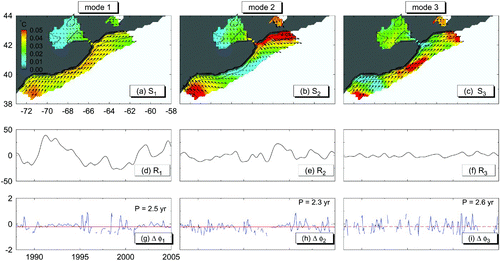
4 The Western Scotian Shelf and Gulf of Maine

The percentages of the total variance explained by the first three CEOFs over this subregion range from 54% to 80% in the three vertical layers (Table 4). Figure 19 presents the spatial and temporal amplitude and phase functions of the first three CEOFs. In contrast to the WNFS-ESS subregion, the first CEOF over this subregion represents onshore (northwestward) propagations of the interannual variability from deep waters to the shelf region as indicated by the spatial phase vectors which rotate clockwise in the onshore direction (Fig. 19a). The first CEOF has large spatial amplitudes off Georges Bank, where anomalies from the Gulf Stream impinge on the shelf (see also Figs 16a and 16b). The second and third CEOFs differ from the first CEOF in that they represent alongshelf advections of anomalies (Figs 19b and 19c). The time-mean periods are about 2.3–2.6 years for the first three CEOFs.

Table 4. Percentages of the total variance explained by the first three CEOFs extracted from the monthly mean temperature and salinity anomalies in the three layers over the subregion of the western Scotian Shelf, the Gulf of Maine and adjacent waters in the control run.

Layer	Percentage of variance
	Temperature			Salinity
	mode 1	mode 2	mode 3	mode 1	mode 2	mode 3
Upper	41.8	18.5	7.5	39.7	17.3	7.2
Intermediate	55.2	20.1	5.1	45.2	18.4	11.9
Lower	51.2	17.5	10.6	36.8	11.1	6.4

Fig. 19 Distributions of spatial amplitude (S ₁) and phase (θ₁;arrows), temporal amplitude (R ₁) and temporal phase change (Δϕ₁) functions of the first (left panels), second (centre panels) and third (right panels) CEOFs for the monthly mean temperature anomalies at 160 m over the western Scotian Shelf and Gulf of Maine region. The red line in the bottom panels represents the averaged temporal phase change.

d Influence of the Gulf Stream on the Interannual Variability over the Scotian Shelf and Slope

As discussed earlier, the non-linear dynamics of the flow play a very important role in driving interannual variability over the eastern Scotian Shelf and the southern Newfoundland Shelf. It was also shown that eddies and anomalies generated by the Gulf Stream or by its interaction with the Labrador Current affect the interannual variability in these regions. To establish the role of the Gulf Stream in the simulated interannual variability, we estimated the Gulf Stream position (GSP) index, along with the shelf-slope front (SSF) index based on model results in Exp-Control.

The GSP index is the (relative) north–south position of the 15°C isotherm at 200 m depth around the Gulf Stream region (Joyce et al., 2000). It should be noted that several different methods have been suggested for calculating the GSP index. For instance, Drinkwater et al. (1994) determined the GSP and the SSF indices based on the positions where the largest SST gradients are encountered in meridional sections crossing the Gulf Stream. Taylor (1996) used a principal component analysis to determine the GSP index. A comparison of the annual-mean GSP and SSF indices from model results (Drinkwater et al., 1994; Joyce et al., 2000) with the indices estimated from remote sensing data for the period 1992–2003 (Han, 2007) is presented in Fig. 20a. Satellite-derived estimates of the GSP index reveal that its range of variability is of the order of 0.8°, with the northernmost positions occuring around 1993 followed by a retreat to its southernmost position by 1996 and then a northward excursion until 2002. The variability displayed by the SSF index is qualitatively similar to that of the GSP index. Also, the model estimated indices match the observed trends of the GSP index having maximum northern excursions around 1992 and 2000 and a maximum southern excursion in 1996–1997.

Fig. 20 (a) Simulated annual-mean Gulf Stream (GSP) and shelf-slope front (SSF) position anomalies for the period 1988–2004 based on the methodologies used by Drinkwater et al. (1994) (SST gradients) and by Joyce et al. (2000) (15°C isotherm). Also shown are the GSP and SSF anomalies estimated from remote sensing data (data from Han (2007)) for the period 1992–2003; (b) standardized monthly time series of the first CEOF of temperature over the eastern Scotian Shelf at 200 m and the simulated GSP anomaly estimated from the position of the 15°C isotherm at 200 m depth.

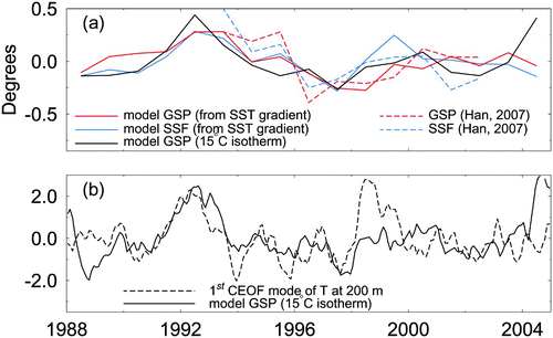
When the Gulf Stream reached its northernmost positions (positive GSP index), the simulated interannual temperature over the Scotian Shelf and Slope region was warmer than during southern shifts of the Gulf Stream. Similarly, during positive GSP index periods the current anomalies along the shelf break and upper slope are in the northeast direction, indicating a reduced equatorward transport by the offshore branch of the Labrador Current. Therefore, there is evidence of connections between the meridional shifts of the Gulf Stream and the interannual variability of currents and hydrography over the Scotian Shelf and Slope Water region. Figure 20b shows the normalized time series of the GSP index and the first CEOF coefficients of interannual temperature anomalies at 200 m over the eastern Scotian Shelf. The interannual variabilities are remarkably similar for the two time series. A correlation analysis between the GSP index and the mode coefficients of the first CEOF reveals a maximum correlation of 0.4, which is statistically significant at the 95% confidence level. It should be noted that more study is needed to examine how the Gulf Stream variability affects the interannual variability over the Slope Water region and the shelf break of the Scotian Shelf.

6 Summary and conclusions

Circulation and hydrography over the eastern Canadian continental shelf (ECS) exhibit large seasonal and interannual variability (Petrie et al., 1992). A numerical investigation based on the NEMO coupled ocean–ice model (Madec, 2008) was conducted in this study to examine the main physical processes affecting the interannual variability over the ECS and adjacent waters using a regional ocean circulation model. The model uses a combination of the spectral nudging method and the smoothed semiprognostic method with smaller-than-usual coefficients for both methods to reduce model seasonal bias and errors. By comparing model results with observations and previous numerical results in the literature, we demonstrated that the regional circulation model reproduces reasonably well the time-means and seasonal cycles in the 3-D circulation and hydrography over the ECS and adjacent waters. The model also has reasonable skill in simulating interannual variability over the ECS.

Four numerical experiments were conducted using the same model setup and parameters but with different combinations of model external forcing to investigate the role of monthly-mean anomalies in the surface forcing, boundary forcing and model internal dynamics, in the interannual variability of the 3-D circulation and hydrographic distributions. The model was integrated for 18 years, from 1987 to 2004, and model results for the last 17 years were presented in this paper. A Complex Empirical Orthogonal Function (CEOF) analysis was used to identify the propagating and standing patterns of interannual variability from the 3-D model results. The CEOF analysis was applied separately to model results over four different subregions of the ECS, mainly because of large regional differences in the 3-D circulation over these subregions.

It was demonstrated that the interannual variability in the model temperature and salinity over the Labrador Shelf and the northern Newfoundland Shelf in the control run was significantly affected by the interannual variability that propagates onto this subregion through the northern open boundary of the model. The interannual variability over the eastern Newfoundland Shelf and adjacent deep waters was also affected by the equatorward advection of the Labrador Current on the shelf and at the shelf edge. Over these two regions, significant correlations between the NAO index and the temperature and salinity anomalies were found with fresher and cooler conditions lagging intense winters (positive NAO index) in the northern hemisphere. Additionally, the variability over the eastern Newfoundland Shelf and adjacent deep waters is affected by the anomalies generated by the non-linear interaction between the equatorward Labrador Current and the poleward North Atlantic Current over the deep water region between the shelf edge of the eastern Grand Banks and the western edge of the North Atlantic Current. Once the anomalies were generated over this region, they moved slowly either poleward (northward) or equatorward (southward), depending on the competing influence of the Labrador Current and the North Atlantic Current. Similar processes also occured for anomalies generated by the Gulf Stream in the deep waters to the south of the Tail of the Grand Banks.

The interannual variability over the western Newfoundland Shelf, Scotian Shelf, and adjacent waters, particularly at the shelf edge of the subregion, is affected by the variability that is advected into this subregion by the equatorward Labrador Current. The correlation between the monthly mean hydrographic anomalies over this subregion and those at the northern open boundary (including Labrador Current anomalies transport), however, is rather low. It was found that the interannual variability in this region has larger amplitudes in the subsurface waters, which is in agreement with Petrie and Drinkwater (1993). The analysis of model results demonstrates that the variability in this subregion, particularly over the Slope Waters off the Scotian Shelf is significantly affected by the anomalies generated by the Gulf Stream, which are entrained into the continental slope of the southern Newfoundland Shelf and advected into this subregion by the Labrador Current. The Gulf Stream and its north–south excursions seem to play a role in the interannual variability of the hydrographic properties, and perhaps transport variability, of the Labrador Current along the shelf-break region south and west of the Grand Banks.

There are two important advective processes that affect the interannual variability of the circulation and hydrography over the western Scotian Shelf and the Gulf of Maine subregion. The first is the onshore propagation of the interannual variability, produced by the Gulf Stream, from deep waters to this subregion in the upper water column of less than 300 m. The second is the equatorward propagation of the interannual variability along the shelf break from the Scotian Shelf to this subregion.

Acknowledgements

We wish to thank Keith Thompson, Helmuth Thomas, Frédéric Dupont, Brian Petrie, Youyu Lu, Yuehua Lin, Shiliang Shan, Paul Mattern and two anonymous reviewers for their useful suggestions and comments. We thank Greg Smith for providing the global ocean reanalysis data. We also want to thank Simon Higginson for providing MSST for the model validation and Igor Yashayaev for providing a schematic of the surface circulation in the north Atlantic. This study was funded by the Global Ocean-Atmosphere Prediction and Predictability project (GOAPP) and the Platform for Ocean Knowledge Management (POKM) project. The work was also supported by The Lloyd's Register Educational Trust (The LRET), which is an independent charity working to achieve advances in transportation, science, engineering and technology education, training and research worldwide for the benefit of all.

References

- Barnier , B. , Madec , G. , Penduff , T. , Molines , J-M. , Treguier , A-M. , Le Somer , J. , Beckmann , A. , Biastoch , A. , Böning , C. , Dengg , J. , Derval , C. , Durand , E. , Gulev , S. , Remy , E. , Talandier , C. , Theetten , S. , Maltrud , M. , McLean , J. and De Cuevas , B. 2006 . Impact of partial steps and momentum advection scheme in a global ocean circulation model at eddy-permitting resolution . Ocean Dyn. , 56 : 543 – 567 . doi:10.1007/s10236-006-0082-1
- Colbourne , E. , deYoung , B. , Narayanan , S. and Helbig , J. 1997 . Comparison of hydrography and circulation on the Newfoundland Shelf during 1990–1993 with the long-term mean . Can. J. Fish. Aquat. Sci. , 54 ( Suppl. 1 ) : 68 – 80 .
- Colbourne , E. and Foote , K. 2000 . Variability of the stratification and circulation on the Flemish Cap during the decades of the 1950s–1990s . J. Northw. Atl. Fish. Sci. , 26 : 103 – 122 .
- Dickson , R. , Meincke , J. , Malmberg , S. and Lee , A. 1988 . The “Great Salinity Anomaly” in the northern North Atlantic 1968–1982 . Prog. Oceanogr. , 20 : 130 – 151 .
- Drinkwater, K.F.; R.A. Myers, R.G. Pettipas and T.L. Wright. 1994. Climatic data for the Northwest Atlantic: The position of the shelf/slope front and the northern boundary of the Gulf Stream between 50°W and 75°W, 1973–1992. Can. Data Rept. Fish. Ocean. Sci. Report No. 125: 103pp. Bedford Institute of Oceanography, Dartmouth, Nova Scotia, Canada.
- Eden , C. , Greatbatch , R. J. and Böning , C. 2004 . Adiabatically correcting an eddy-permitting model using large-scale hydrographic data: Application to the Gulf Stream and the North Atlantic Current . J. Phys. Oceanogr. , 34 : 701 – 719 .
- Fuglister , F. and Worthington , L. 1951 . Some results of a multiple ship survey of the Gulf Stream . Tellus, , 3 : 1 – 14 .
- Gaspar , P. , Grégoris , P. and Lefevre , J.-M. 1990 . A simple eddy kinetic energy model for simulations of the oceanic vertical mixing tests at Station Papa and long-term upper ocean study site . J. Geophys. Res. , 96 : 16179 – 16193 .
- Gatien , M. G. 1976 . A study in the slope water region south of Halifax . J. Fish. Res. Board of Can. , 33 : 2213 – 2217 .
- Geshelin, Y.; J. Sheng and R.J. Greatbatch. 1999. Monthly mean climatologies of temperature and salinity in the western North Atlantic. Can. Data Rep. Hydrogr. Ocean Sci. Report No. 153, 62 pp. Bedford Institute of Oceanography, Dartmouth, Nova Scotia, Canada.
- Gill , A. 1982 . Atmosphere-Ocean Dynamics , San Diego : Academic .
- Greatbatch , R. J. , Sheng , J. , Eden , C. , Tang , L. and Zhai , X. 2004 . The semi-prognostic method . Cont. Shelf Res. , 24 : 2149 – 2165 .
- Griffies , S. and Hallberg , R. 2000 . Biharmonic friction with a Smagorinsky-like viscosity for use in large-scale eddy-permitting ocean models . Mon. Weather Rev. , 128 : 2935 – 2946 .
- Hachey, H.B.; F.F. Hermann and W.B. Bailey. 1954. The waters of the ICNAF convention area. In Proc. Int. Comm. Northwest Atl. Fish. Ann. Proc. Vol. 4, pp. 67–102. 8 October 1953, Copenhagen, Denmark.
- Han , G. 2007 . Satellite observations of seasonal and interannual changes of sea level and currents over the Scotian Slope . J. Phys. Oceanogr. , 37 : 1051 – 1065 .
- Han , G. and Tang , C. L. 2001 . Interannual variations of volume transport in the western Labrador Sea based on TOPEX/Poseidon and WOCE data . J. Phys. Oceanogr. , 31 : 199 – 211 .
- HAN, G. and J.W. LODER. 2003. Three-dimensional seasonal-mean circulation and hydrography on the eastern Scotian Shelf. J. Geophys. Res. 108(C5): 1–21.
- HAN, G.; Z. LU, Z. WANG, J. HELBIG, N. CHEN and B. DEYOUNG. 2008. Seasonal variability of the Labrador Current and shelf circulation off Newfoundland. J. Geophys. Res. 113: C10013, doi;10.1029/2007JC004376
- Hannachi , A. , Jolliffe , I. T. and Stephenson , D. B. 2007 . Empirical orthogonal functions and related techniques in atmospheric science: A review . Int. J. Climatol. , 27 : 1119 – 1152 .
- Hannah , C. G. , Shore , J. A. , Loder , J. W. and Naime , C. E. 2001 . Seasonal circulation on the western and central Scotian Shelf . J. Phys. Oceanogr. , 31 : 591 – 615 .
- Head , E. and Sameoto , D. 2007 . Inter-decadal variability in zooplankton and phytoplankton abundance on the Newfoundland and Scotian shelves . Deep-Sea Res. , 54 : 2686 – 2701 . doi:10.1016/j.dsr2.2007.08.003
- Higginson , S. , Thompson , K. R. , Huang , M. , Véronneau , M. and Wright , D. 2011 . The mean surface circulation of the North Atlantic subpolar gyre: A comparison of estimates derived from new gravity and oceanographic measurements . J. Geophys. Res. , 116 CO8016, A.R. Robinson and K.H. Brink (eds) doi:10.1029/2010JC006877
- Horel , J. D. 1984 . Complex principal component analysis: Theory and examples . J. Clim. Appl. Meteorol. , 23 : 1660 – 1673 .
- Joyce , T. M. , Deser , C. and Spall , M. A. 2000 . The relation between decadal variability of subtropical mode water and the North Atlantic Oscillation . J. Clim. , 13 : 2550 – 2569 .
- Large , W. and Pond , S. 1981 . Open ocean momentum flux measurements in moderate to strong winds . J. Phys. Oceanogr. , 11 : 324 – 336 .
- Large, W. and S. Yeager. 2004. Diurnal to decadal global forcing for ocean and sea-ice models: The data sets and flux climatologies. Tech. Report TN-460+STR, NCAR, 105 pp. Boulder, Colorado, USA.
- Lazier , J. and Wright , D. 1993 . Annual velocity variations in the Labrador Current . J. Phys. Oceanogr. , 23 : 659 – 678 .
- Loder , J. W. , Petrie , B. and Gawarkiewicz , G. 1998 . “ The coastal ocean off northeastern North America: A large-scale view. In ” . In The Sea. Vol 11., The Global Coastal Studies. Regional Studies and Syntheses , Edited by: Robinson , A. R. and Brink , K. H. 105 – 133 . USA : John Wiley & Sons, Inc .
- Lynch , D. R. , Ip , J. T.C. , Naime , C. E. and Werner , F. E. 1996 . Comprehensive coastal circulation model with application to the Gulf of Maine . Cont. Shelf Res. , 16 : 875 – 906 .
- Madec, G. 2008. NEMO Reference Manual, Ocean Dynamics Component: NEMO-OPA, Preliminary Version. Note du Pole de modélisation, Institute Pierre Simon Laplace (IPSL), France, No 27 ISSN: 1288–1619.
- Marchesiello , P. , McWilliams , J. and Shchepetkin , A. 2001 . Open boundary conditions for long term integration of regional oceanic models . Ocean Modelling, , 3 : 1 – 20 .
- Marsh , R. , Petrie , B. , Weidman , C. , Dickson , R. , Loder , J. , Hannah , C. , Frank , K. and Drinkwater , K. 1999 . The 1882 tilefish kill - a cold event in shelf waters off the north-eastern United States? . Fish. Oceanogr. , 8 : 39 – 49 .
- McLellan , H. J. 1957 . On the distinctness and origin of the slope water off the Scotian Shelf and its easterly flow south of the Grand Banks . J. Fish. Res. Board Can. , 14 : 4213 – 4239 .
- Niiler , P. 2001 . “ The world ocean surface circulation ” . In Ocean Circulation and Climate – Observing and Modelling the Global Ocean , Edited by: Church , J. , Siedler , G. and Gould , J. 193 – 204 . London : Academic .
- Petrie , B. 2007 . Does the North Atlantic Oscillation affect hydrographic properties on the Canadian Atlantic continental shelf? . Atmosphere-Ocean, , 45 : 141 – 151 .
- Petrie , B. and Anderson , C. 1983 . Circulation on the Newfoundland Shelf . Atmosphere-Ocean, , 21 : 207 – 226 .
- Petrie , B. , Loder , J. W. , Lazier , J. and Akenhead , S. 1992 . Temperature and salinity variability on the eastern Newfoundland Shelf: The residual field . Atmosphere-Ocean, , 30 : 129 – 139 .
- Petrie , B. and Drinkwater , K. 1993 . Temperature and salinity variability on the Scotian Shelf and the Gulf of Maine 1945–1990 . J. Geophys. Res. , 98 : 20079 – 20089 .
- Pickart , R. and Smethie , W. Jr . 1998 . Temporal evolution of the deep western boundary current where it enters the subtropical domain . Deep-Sea Res. , 45 : 1053 – 1083 .
- Shadwick , E. , Thomas , H. , Comeau , A. , Craig , S. , Hunt , C. and Salisbury , J. 2010 . Air-sea CO2 fluxes on the Scotian Shelf: seasonal to multi-annual variability . Biogeosciences, , 7 : 3851 – 3867 .
- Sheng , J. and Thompson , K. R. 1996 . A robust method for diagnosing regional shelf circulation from scattered density profiles . J. Geophys. Res. , 101 : 25647 – 25659 .
- Sheng , J. , Greatbatch , R. J. and Wright , D. G. 2001 . Improving the utility of ocean circulation models through adjustment of the momentum balance . J. Geophys. Res. , 106 : 16711 – 16728 .
- Sheng , J. and Tang , L. 2003 . A numerical study of circulation in the western Caribbean Sea . J. Phys. Oceanogr. , 31 : 3146 – 3163 .
- Smith , G. C. , Haines , K. , Kanzow , T. and Cunningham , S. 2010 . Impact of hydrographic data assimilation on the modelled Atlantic meridional overturning circulation . Ocean Sci. , 6 : 761 – 774 .
- Smith , P. and Schwing , F. 1991 . Mean circulation and variability on the eastern Canadian continental shelf . Cont. Shelf Res. , 11 : 977 – 1010 .
- Smith , R. D. , Maltrud , M. E. , Bryan , F. O. and Hecht , M. W. 2000 . Numerical simulation of the North Atlantic Ocean at 1/10° . J. Phys. Oceanogr. , 30 : 1532 – 1561 .
- Smith , W. H.F. and Sandwell , D. T. 1997 . Global sea floor topography from satellite altimetry and ship depth soundings . Science, , 277 : 1957 – 1962 .
- Stevens , D. 1990 . On open boundary conditions for three dimensional primitive equations ocean circulation models . Geophys. Astrophys. Fluid Dyn. , 51 : 103 – 133 .
- Taylor , A. H. 1996 . North-south shifts of the Gulf Stream: ocean-atmosphere interactions in the North Atlantic . Int. J. Climatol. , 16 : 559 – 583 .
- Terradas , J. , Oliver , R. and Bellester , J. L. 2004 . Application of statistical techniques to the analysis of solar coronal oscillations . Astrophys. J. , 614 : 435 – 447 .
- Thompson , K. R. , Lazier , J. R.N. and Taylor , R. 1986 . Wind-forced changes in Labrador Current transport . J. Geophys. Res. , 91 : 14261 – 14268 .
- Thompson , K. R. , Loucks , R. H. and Trites , R. W. 1988 . Sea surface temperature variability in the shelf-slope region of the northwest Atlantic . Atmosphere-Ocean, , 26 : 292 – 299 .
- Thompson , K. R. , Wright , D. G. , Lou , Y. and Demirov , E. 2006 . A simple method for reducing seasonal bias and drift in eddy resolving ocean models . Ocean Modelling, , 13 : 109 – 125 .
- Thompson , K. R. , Ohashi , K. , Sheng , J. , Bobanovic , J. and Ou , J. 2007 . Suppressing bias and drift of coastal circulation models through the assimilation of seasonal climatologies of temperature and salinity . Cont. Shelf Res. , 27 : 1303 – 1316 .
- Timmermann , R. , Goosse , H. , Madec , G. , Ficheft , T. , Ethe , C. and Duliere , V. 2005 . On the representation of high latitude processes in the ORCA-LIM global coupled sea ice-ocean model . Ocean Modelling, , 8 : 175 – 201 .
- Trossman , D. S. , Thompson , L. , Kelly , K. A. and Kwon , Y-O. 2009 . Estimates of North Atlantic ventilation and model water formation for winters 2002–06 . J. Phys. Oceanogr. , 39 : 2600 – 2917 .
- Weare , B. C. 1977 . Empirical orthogonal function analysis of Atlantic Ocean surface temperature . Q. J. R. Meteorol. Soc. , 103 : 467 – 478 .
- Wright , D. G. , Thompson , K. R. and Lu , Y. 2006 . Assimilating long-term hydrographic information into an eddy-permitting model of the north Atlantic . J. Geophys. Res. , 111 doi:10.1029/2005JC003200
- Xue , H. , Chai , F. and Pettigrew , N. 2000 . A model study of the seasonal circulation in the Gulf of Maine . J. Phys. Oceanogr. , 30 : 1111 – 1135 .
- Zhao , J. , Sheng , J. , Greatbatch , R. J. , Azetsu-Scott , K. and Jones , E. P. 2006 . Simulation of CFCs in the North Atlantic Ocean using an adiabatically corrected ocean circulation model . J. Geophys. Res. , 111 : C06027 doi:10.1029/2004JC002814