Electric Load Forecasting for Western Canada: A Comparison of Two Non-Linear Methods

Abstract

Seven years of hourly temperature and electric load data for British Columbia in western Canada were used to compare two statistical methods, artificial neural networks (ANN) and gene expression programming (GEP), to produce hour-ahead load forecasts. Two linear control methods (persistence and multiple linear regression) were used for verification purposes. A two-stage (predictor-corrector) approach was used. The first stage used a single regression model that applied weather and calendar data for the previous hour to predict load for any hour of the day, and the second stage applied different corrections every hour, based on a high correlation of today's load with yesterday's load for any given hour. By excluding the day-before variables, the two-stage method reduced the total number of variables in the first-stage regression and gave better results. The first five years of data were used for training (regression finding) and validation (comparative testing of candidate functions to reduce overfitting) and the last two for verification (scoring with independent data).

It was found that both non-linear methods worked better than the linear methods for the first stage. All methods worked well for the second stage; hence, persistence is recommended for the second stage because it is easiest to do. After both stages, the load error was less than 0.6% of the load magnitude for hour-ahead forecasts. When used iteratively to create forecasts up to 24 hours ahead, errors grew to about 3.5% of the load magnitude for both GEP and ANNs. We also experimented by training the statistical methods with a shorter period (one year) of past data to examine the over-fitting problem. Overall, ANNs were more useful in fitting the curves to robust data, and GEP was superior for short datasets and was less sensitive to the length of the dataset. We also found that a time-nested electric load forecasting model with different lead times kept maximum load errors to 2.1% of the load magnitude out to a horizon of 24 forecasts.

RÉSUMÉ [Traduit par la rédaction] Nous avons utilisé sept années de données de température et de charge électrique pour la Colombie-Britannique dans l'ouest du Canada pour comparer deux méthodes statistiques, les réseaux neuronaux artificiels (ANN) et la programmation génétique (GEP), pour produire des prévisions de charge une heure à l'avance. Nous nous sommes servis de deux méthodes de vérification linéaires (persistance et régression linéaire multiple) à des fins de vérification. Nous avons utilisé une approche en deux étapes (prédicteur–correcteur). Dans la première étape, un modèle de régression simple appliquait des données météorologiques et de calendrier pour l'heure précédente pour prévoir la charge à n'importe quelle heure de la journée et la deuxième étape appliquait à chaque heure différentes corrections basées sur une forte corrélation de la charge d'aujourd'hui avec la charge d'hier pour une heure quelconque. En excluant les variables du jour précédent, la méthode à deux étapes a réduit le nombre total de variables dans la régression de la première étape et a donné de meilleurs résultats. Nous avons utilisé les cinq premières années de données pour l'apprentissage (détermination de la régression) et la validation (essais comparatifs de fonctions candidates pour réduire le surapprentissage) et les deux dernières pour la vérification (établissement d'un score à l'aide de données indépendantes).

Il ressort que les deux méthodes non linéaires ont mieux fonctionné que les méthodes linéaires pour la première étape. Toutes les méthodes ont bien fonctionné pour la deuxième étape; la persistance est donc recommandée pour la deuxième étape parce qu'elle est plus facile à appliquer. Après les deux étapes, l'erreur sur la charge était inférieure à 0,6% de la grandeur de la charge pour les prévisions d'une heure à l'avance. Lorsque utilisées de façon itérative pour produire des prévisions de jusqu’à 24 heures, les erreurs ont augmenté jusqu’à environ 3,5% de la grandeur de la charge tant pour la GEP que les ANN. Nous avons aussi expérimenté en entraînant les méthodes statistiques avec une période plus courte (un an) de données passées pour examiner le problème du surapprentissage. Dans l'ensemble, les ANN étaient plus utiles pour ajuster les courbes aux données robustes alors que la GEP était meilleure pour les courts ensembles de données et était moins sensible à la longueur de l'ensemble de données. Nous avons aussi trouvé qu'un modèle de prévision de charge électrique emboîté dans le temps avec différent temps de prévision a limité les erreurs sur la charge à 2,1% de la grandeur de la charge jusqu’à un horizon de 24 prévisions.

Keywords:

• genetic programming
• electric load forecasting
• artificial neural networks
• gene expression programming

1 Introduction

Electrical load forecasting has been a major concern in applied meteorology for many years. Studies on mathematical and heuristic techniques, input variable selection and verification have already been extensively published in literature by other researchers (Alfares and Nazeeruddin, 2002; Fildes et al., 2008; Hinojosa and Hoese, 2010).

Genetic programming, which allows algorithms to evolve until they fit a dataset, has been used for a wide variety of scientific and engineering applications (Holland, 1975; Cramer, 1985; Koza, 1992). A new variant, called gene expression programming (GEP; Ferreira, 2006), is very efficient at finding solutions. GEP has been used in load forecasting (Sadat Hosseini and Gandomi, 2010; Bakhshaii and Stull, 2011), numerical weather prediction (Bakhshaii and Stull, 2009; Roebber, 2010; Stull, 2011), hydrology (Aytek et al., 2008) and many other fields in recent years. This work examines hourly electrical load forecasting using GEP and artificial neural networks (ANN).

ANN modelling is well established as a tool for electric load forecasting, both as a stand-alone tool (da Silva and Moulin, 2000; Hippert et al., 2001; Mori and Yuihara, 2001; Marin et al., 2002; Taylor and Buizza, 2002; Beccali et al., 2004; Hippert and Pedreira, 2004; Musilek et al., 2006; Hinojosa and Hoese, 2010) and as a hybrid (Khotanzad et al., 1998; Srinivasan et al., 1999; Huang and Yang, 2001; Ling et al., 2003; Chen et al., 2004; Fan and Chen, 2006; Liao and Tsao, 2006; Amjady, 2007; Yun et al., 2008; Bashir and El-Hawary, 2009). While the ANN node-connection diagram is relatively simple (Hsieh, 2009), users might forget that a very large number of free parameters must be determined for ANNs. This large number of parameters/weights is both an advantage and a disadvantage. As an advantage, it enables ANNs to fit very complex non-linear behaviours. As a disadvantage, it often means that care must be taken to pick parameters that fit the signal and not the noise (Hippert et al., 2001; Osowski and Siwek, 2002; Chan et al., 2006; Ferreira, 2006; Mao et al., 2009; Hinojosa and Hoese, 2010).

Because GEP is not widely known in the atmospheric community, we explain it in detail in Section 2. Section 3 describes the data. Section 4 gives the procedure for making one-hour-ahead load forecasts and that procedure is verified with independent data in Section 5. In Section 6 we iteratively extend the forecast to 24 hours ahead, and Section 7 examines using a shorter length of training data. A summary with conclusions appears in the last section.

2 Gene expression programming

a Overview of the Basic Genetic Programming Procedure

The procedure is to first create a “world” with a population of randomly created candidate algorithms that relate electric load to predictors such as weather. Next, the fitness of each candidate is found by verifying its load forecasts against a “training” data subset. Then the candidates that survive (some with a mutation and interchange of genetic information) into the next generation are selected—a selection process that favours the more fit individuals but maintains diversity. The new generation of algorithms are selected and the selection process is invoked again. After many generations the best verification score plateaus. The resulting relative winner is saved.

This process should be repeated to create different initial worlds using the same procedure described above; this allows different evolutionary paths to be followed to produce different relative winners. It is recommended that a different subset of data be used to “validate” and compare each relative winner in order to select the one winner that has the best overall fitness statistics with the least overfitting. These validation data are also known as “testing” data by the author of GEP (Ferreira, 2006).

The final statistics of the overall winner should be evaluated using a third data subset, known as “verification” data to the meteorological community, or as “scoring” data in the GEP community (Ferreira, 2006). The three data subsets (training, validation/testing, and verification/scoring) help reduce overfitting and ensure independent verification of the final electric-load algorithm. The specific methods used by GEP to achieve this computational selection are described next.

b Specific Concepts of Gene Expression Programming

By analogy with biology, a candidate electrical-load-estimating algorithm is called an individual. The genetic information (i.e., the genotype, but called the genome in GEP literature) for an individual is encoded in a chromosome. The chromosome can consist of one or more genes. Each gene is a linear string of characters.

Each gene is divided into a head and a tail. In the head are characters representing basic functions (+, −, *, /, ln, sin, conditionals, etc.), predictors (e.g., meteorological variables, past load, calendar flags), and numbers (e.g., weights). Only predictors and numbers are in the tail. During evolution, no functions or operators are ever allowed into the tail. This artificial division into a head and tail ensures that there will always be sufficient arguments (predictors or weights) for each operator or function in the head to operate on, regardless of the amount of mutation of the head. For this to work, the head length (h) is fixed, and the tail size is computed as tail = h (n _max − 1) + 1, where n _max is the maximum arity. Arity is the number of arguments that an operator or function can take.

As the evolution progresses and individuals with different genotypes are created, these individuals can have different gene lengths. The genes are combined into chromosomes using a simple arithmetic operator such as +, −, *, or /. We used addition for this study.

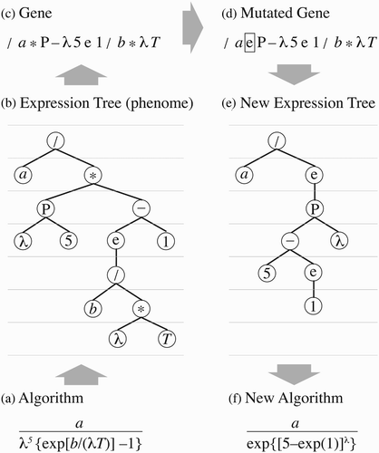
Figure 1 shows an example of how a mathematical algorithm can be represented by a genotype and how mutation in this genotype produces a new algorithm. What makes GEP different from previous genetic programming methods is that the genome is coded by reading the expression tree like a book, rather than by following the node connections. Decoding back to an algorithm is possible because the arity of each operator and each basic function are known (Ferreira, 2006; Bakhshaii and Stull, 2009). The read-like-a-book coding is the key to the efficiency of GEP, because every mutation gives a viable individual (i.e., a mathematical expression that can be evaluated).

Fig. 1 Illustration of GEP coding. (a) Planck's law as a mathematical formula. The variables are wavelength λ and temperature T, and the Planck constants are a and b. (b) Expression-tree representation (the phenome: physical representation). The basic operators are (*, /, −), and the basic functions are power function P(x,y) = x^y , and e representing exp(x). (c) GEP coding (the gene: info that describes the phenome). The code is created by reading the expression tree as a book (i.e., not following the node connections but reading each line from left to right, from the top line to the bottom). (d) Mutation of the third character in the gene. (e) New expression tree built from the mutated gene. This is possible because the arity of each basic function is known (e.g., P takes two arguments, but e takes only one.) (f) The corresponding new mathematical formula.

Mutation (change of a randomly chosen character in the gene) is the most effective modification of the chromosome. Computational evolution is accelerated relative to biological evolution (Ferreira, 2006) by using a mutation rate of 0.044 (i.e., 44 mutations per 100-character chromosome per 10 generations). Mimicking biology, the following additional modification methods are also randomly invoked in GEP:

•	Inversion—reversing the character order in a random substring; rate = 0.1
•	Insertion sequence transposition—a random substring moves to a different random location; rate = 0.1
•	Root insertion sequence transposition—a random substring moves to the front of the gene; rate = 0.1
•	Gene transposition—an entire randomly chosen gene moves to the front of the chromosome; rate = 0.1
•	One-point recombination—swapping of trailing substrings from identical starting locations between two genes; rate = 0.3
•	Two-point recombination—swapping substrings between the same start and end points in two chromosomes; rate = 0.3
•	Gene recombination—randomly selected entire genes are swapped between two individuals; rate = 0.1

Selection of survivors is done by computationally mimicking a roulette wheel that has as many segments as the population. However, the size of each segment is proportional to the fitness of each individual. The wheel is “spun” as many times as the size of the population, and the winners are retained into the next generation. Thus, the total population count is constant. This roulette-wheel selection favours the fittest individuals but still retains some less fit individuals to help maintain genetic diversity. Ferreira (2006) compares roulette-wheel selection with tournament selection and deterministic selection (where selection is proportional to fitness) and recommends roulette-wheel selection because it has a high success rate with reduced computer time for complex real-world problems.

The user of GEP is free to decide the basic functions that can be used in the gene and the number of basic functions and weights allowed in the algorithm. Consider the following trade-offs when selecting the choice of basic functions. If a small number of basic functions are chosen, then a longer chromosome might be needed to achieve a fit to the data with the desired accuracy. Alternatively, by allowing GEP to choose from a larger number of more complex functions, the same accuracy might be achieved with a shorter chromosome.

Both approaches often yield similar overall complexities. If the data to be fitted are simple enough, then it is beneficial to have a small choice of basic functions and a short chromosome (Roebber, 2010) because the functional form can be more easily interpreted by humans. A sample of a load forecast algorithm created by GEP is shown in the Appendix.

3 Data

The area for the case study is British Columbia (BC), Canada, located between the Pacific coast of North America and the Rocky Mountains. BC is 950,000 km² and is characterized by high mountains (2000 to 3000 m), deep narrow valleys, coastlines, fjords, glaciers and interior plateaus. The climate in BC varies from mild marine coastal Mediterranean to hot semi-arid.

BC Hydro provides electricity to 94% of the province's 4.5 million people. About 70% to 85% of BC Hydro's electricity is consumed in Metro Vancouver, a city of about two million people in the southwest corner of BC. For this reason, and following BC Hydro's operational practice, we used temperature at Vancouver International Airport (CYVR) as the only weather input for this focused study. Although this is counterintuitive, it gave better load forecasts than using more weather variables such as dew-point temperature, wind speed or other weather conditions.

Hourly temperature and electrical load data were used for the case study period 1 January 2004 to 31 December 2010. This seven-year period was divided into training, testing (validation), and scoring (verification) segments. The first 5.25 years of load and weather data (1 January 2004 to 31 March 2009) were randomly divided into two portions—80% for training and 20% for testing (validation). The GEP used the testing (validation) data to find the overall winner from multiple worlds of evolution, while the ANN used the testing data to stop the regression when overfitting began. The remaining data (1 April 2009 to 31 December 2010) were used as independent data to score (verify) the results. All of the verifying graphs, tables and statistical results in Sections 5 to 7 are based on this independent portion of data.

As a “perfect prog” experiment, we used ex post facto observed temperatures as input to the regressions; hence, we evaluated only the quality of the load regressions and not the quality of the weather forecasts. Advantages of the perfect prog approach are that it is independent of the source of the weather data, so any changes in operational weather forecasting models or in humans that provide adjusted weather inputs do not require GEP or ANN regressions to be re-computed. The disadvantage is that the regression does not correct for systematic errors in the weather variables. But this is actually an advantage, because weather forecasts should have their own model output statistics (MOS) postprocessing to correct systematic errors, instead of this weather correction being confounded with the electric load regression.

4 Procedure for one-hour-ahead load forecasts

a Stage 1: Load Forecast

To forecast the electric load L(t + 1) predictand for a valid time of one hour in the future, we used the following six predictors as input:

•	present load L(t)
•	present temperature T(t)
•	forecast temperature T(t + 1) at the valid time
•	month index M(t + 1) at the valid time
•	code for day of the week D(t + 1) at the valid time
•	hour H(t + 1) at the valid time

where the month code is M = 01, 02, … , 11, 12 for January to December, respectively; the hour code is H = 01, 02, … , 23, 24, and the code for the day of the week is D = 1, 2, … , 6, 7, 9 for Sunday, Monday, … , Friday, Saturday, holidays, respectively.

As reported by others (Khotanzad et al., 1998; Bashir and El-Hawary, 2009; Hinojosa and Hoese, 2010), we also found that the best fits occurred when the data were first split into three categories: weekdays (Monday–Friday), weekends (Saturday and Sunday), and holidays. Separate regressions were done using each statistical method for each category. The day code was not used for holidays, because all holidays share the same code of 9.

For stage 1 (the predictor stage), we intentionally did not find separate models/regressions for each hour of the day. Instead, we found the regression that gave a one-hour-ahead forecast, based on a model that was trained using all hours in any one category such as weekdays. Our preliminary experiments showed that even though this approach yielded load forecasts with substantial errors after stage 1, the load errors were very highly correlated from one day to the next. Other researchers have used the weather and load variables of a day-before forecast day to circumvent this issue (Drezga and Rahman, 1998; Khotanzad et al., 1998; Taylor and Buizza, 2002). Based on these preliminary experiments, we hypothesized that a two-stage (predictor-corrector) approach could yield accurate forecasts with relatively few free parameters.

We compared two different methods to create the statistical relationship between predictors and predictand: GEP

and ANN

where the subscript 1 denotes the first stage in this procedure.

As a baseline we compared the results of the non-linear methods with the results from two linear methods: multiple linear regression (MLR)

and persistence (PER)

GEP is programmed to use the following functions and operators: +, −, *, /, exp, ln, ()², ()³, ()^1/2, ()^1/3, sin, cos and arctan. The first four of these operators have an arity (number of arguments) of 2, and the next nine have an arity of 1. The multigenic chromosome used five genes, each gene having a head size of 8 and length of 25 (Ferreira, 2006). An algorithm produced by GEP is illustrated in the Appendix.

ANN is programmed as a feed-forward, back propagation network (Taylor and Buizza, 2002) with an input layer of 6 nodes, one hidden layer of 10 nodes and an output layer of 1 node. This ANN required that 81 free parameters be determined. We experimented with different counts of nodes in the hidden layer. As the node count increased past 10, the improvement in verification errors plateaued. Hence, we used 10 hidden nodes for this study. ANN uses a hyperbolic tangent sigmoid transfer function [y = 2/(1 + exp (−2x)) −1] on the input and a linear transfer function on the output.

MLR solves a set of simultaneous equations to give the weights for a least-squares best fit between observed loads and the weighted sum of predictors for the training data. For PER we assume that the load forecast is the same as the present load.

b Interim Behaviour: Motivation for a Second Stage

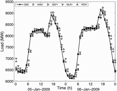
Figure 2 shows a small sample of the single-stage, one-hour-ahead load forecasts during the training period. All the methods (both non-linear and linear) capture the first-order signal, namely, the proper order of magnitude (5000 to 10000 MW) and typical variations during the day (e.g., peaks in late morning and early evening).

Fig. 2 A two-day sample showing observed (OBS) versus forecast loads using only the first stage of regressions. These forecasts are based on stage-1 regressions that were trained on the full multi-year training dataset.

We defined a load error E for any hour (t + 1) as

where F is the forecast value from the load-forecast stage, V is the verifying observation at that hour and the subscript 1 still denotes the first stage. All four statistical methods have roughly the same errors: on the order of plus or minus a few hundred megawatts (see a sample of four methods in Fig. 3). Of these four methods, persistence has the greatest errors. An interesting pattern is observed in the errors that points to even further improvement.

Fig. 3 Load-forecast error versus hour of the day, for every weekday in every January of the training dataset, after stage 1. (a) GEP₁, (b) ANN₁, (c) MLR₁ and (d) PER₁.

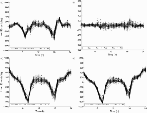
When all weekday errors are plotted versus hour of the day (Fig. 3) for any month in the training period, a recurring error pattern is evident for GEP₁. Namely, the error for any hour is strongly correlated with the errors for that same hour on most other days in that same month for the same category (weekday, weekend). For example, in Fig. 3a, at 0700 local time in January almost every day has an error in the range of −500 to −300 MW, while at 2000 local time most errors are in the range of +200 to +400 MW. Hence, we can use this correlation to reduce errors further, via a bias correction second stage.

To our surprise, the results of incorporating the day-before load as an additional predictor in stage 1 (not shown here) were not as good as the results from the two-stage method. This characteristic is true for both GEP and ANN. So this study focused on the two-stage method.

Note that ANN₁ has substantially lower errors (Fig. 3b) after stage 1 than the other methods for weekdays and weekends. Also, these errors do not exhibit a strong correlation from one day to the next. This confirms that the more complex model (ANN) with more free parameters (81 free weights for our ANN with 10 nodes in the hidden layer) performs better than the simpler models (GEP has up to 10 free weights, MLR has 6 free weights and PER has zero free weights in our implementation). We intentionally did not test more complex forms of GEP and MLR with more free weights because we wanted to evaluate the capability of lower order regressions.

c Stage 2: Recurring Bias Correction

Figure 3 suggests that the error for any hour today should be nearly equal to the error yesterday during that same hour for ANN₁, GEP₁, MLR₁ and PER₁. The simplest such correction would use persistence (PER); namely, assume the bias E(t + 1) for any hour later today is exactly equal to yesterday's bias E(t + 1–24) for the same hour. Alternatively, we could use yesterday's bias as one of the predictors in a second regression stage, which would be a seventh predictor.

We compared bias corrections using the following statistical methods:

where subscript 2 denotes the second stage. So the approach in stage 2 is to find separate regressions (or use separate persistence values) for each hour.

With four statistical methods for stage 1 and four methods for stage 2, there are 16 different combinations that could be tested. We tested the following subset of seven combinations:

•	ANN1-ANN2
•	GEP1-GEP2
•	MLR1-MLR2
•	ANN1-PER2
•	GEP1-PER2
•	MLR1-PER2
•	PER1-PER2

This subset was chosen because it would likely span the range of outcomes.

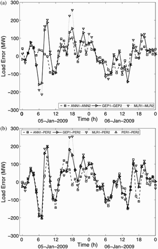
Figure 4 shows the remaining error after using this two-stage process for the same two-day sample as in Fig. 2. The remaining error is reduced to plus or minus a few tens of megawatts. Namely, the mean absolute error is of order 0.6% of the total electric load.

Fig. 4 Two-day sample of errors after both regression stages: (a) ANN₁-ANN₂, GEP₁-GEP₂ and MLR₁-MLR₂; and (b) ANN1₁-PER₂, GEP1-PER₂, MLR1₁-PER₂ and PER₁-PER₂.

To recapitulate, the statistical regressions for stages 1 and 2 were trained and tested using the whole 5.25 years of training data. For stage 1, the predictor stage, each statistical model was trained using every hour of the day. Namely, there was just one MLR model that applied to all weekday hours, one MLR for all weekend hours, one GEP for all weekday hours, etc. Then for stage 2, the corrector stage, separate regressions were created for each hour of the day for each category (except holidays), where the number of data samples for training and testing each of these categories (weekdays, weekends, holidays) was 31560, 13104 and 1320, respectively. These regressions will be verified against the remaining 1.75 years of independent data, with results given in the next section.

5 One-hour-ahead forecast verification using independent data

The best-fit regressions determined from the training data in the previous section were used with no change to predict the load for the independent subset of data. Each of the seven combinations of first and second stages was verified (scored) separately within each category for the independent dataset for 1 April 2009 to 31 December 2010. The number of verification data points for each category (weekdays, weekends, holidays) was 10512, 4344 and 480, respectively.

We also compared the results from these seven combinations with the operational one-hour-ahead load forecasts provided by BC Hydro. We caution the reader that we had no control over the conditions under which these operational values were determined. BC Hydro runs the commercially available Artificial Neural Network Short Term Load Forecaster (ANNSTLF), which utility companies can obtain from the US Electric Power Research Institute (EPRI, 2009). Although BC Hydro inputs forecast temperatures into ANNSTLF for their real-time operational runs, they later go back and re-run ANNSTLF with the ex post facto observed temperatures; then they archive the resulting load “forecasts”. We used these archived (based on observed temperatures) ANNSTLF one-hour-ahead load forecasts as a benchmark against which we measured the success of the proposed methods.

For the verification statistics, F_i is the forecast value for data point i from any of the statistical methods; V_i is the corresponding verifying observation, and the overbar indicates an average over all N data points. The error is E_i  = F_i  − V_i and the mean error (bias) is

The error standard deviation is

The mean absolute error is

The Pearson product-moment correlation coefficient is

where the product of individual standard deviations σ is

Recall that r ² equals the portion of the total variance explained by the regression.

Comparison of Tables 1 and 2 shows that all seven combinations of methods were improved by including the second stage. The linear methods MLR₁-MLR₂, MLR₁-PER₂, and PER₁-PER₂ explained between 95.3% and 99.7% of the variance. The methods with a non-linear first stage and any second stage (GEP₁-GEP₂, ANN₁-ANN₂, ANN₁-PER₂, GEP₁-PER₂) explained between 99.1% and 99.7% of the total variance. For the two-stage methods with a non-linear first stage, the mean absolute errors ranged from 41 to 76 MW. Thus, the two-stage methods used here with a non-linear first stage have better verification statistics than BC Hydro's operational version of ANNSTLF (explained variance of 95.6% to 98.9% with an MAE of 81 to 164 MW, for this dataset).

Table 1. Verification statistics on independent data after both stages.

1 April 2009 to 31 December 2010, 1-hour Load Forecasts	ME (MW)	MAE (MW)	STD (MW)	r ^2
GEP1-GEP2
Week Days	−0.32	42	57	0.997
Weekends	0.11	48	67	0.995
Holidays	−5.0	68	96	0.991
GEP1-PER2
Weekdays	0.02	44	61	0.997
Weekends	0.11	53	73	0.995
Holidays	−5.0	68	96	0.991
ANN1-ANN2
Weekdays	5.67	41	56	0.997
Weekends	2.33	40	55	0.997
Holidays	25.8	76	98	0.991
ANN1-PER2
Weekdays	0.01	45	63	0.997
Weekends	−0.08	48	67	0.995
Holidays	25.8	76	98	0.991
PER1-PER2
Weekdays	−0.03	43	60	0.998
Weekends	−0.10	56	74	0.994
Holidays	4.71	174	219	0.953
MLR1-PER2
Weekdays	−0.07	54	73	0.995
Weekends	−0.18	65	86	0.992
Holidays	3.73	170	212	0.955
MLR1-MLR2
Weekdays	−1.36	51	68	0.996
Weekends	0.06	61	81	0.993
Holidays	3.74	170	212	0.955
ANNSTLF
Weekdays	−2.66	83	114	0.989
Weekends	−6.23	81	114	0.986
Holidays	−4.48	164	218	0.956

Table 2. Verification statistics on independent data for the first stage.

April 2009 to 31 December 2010, 1-hour Load Forecasts	ME (MW)	MAE (MW)	STD (MW)	r ^2
ANN1
Weekdays	9.2	51	70	0.996
Weekends	11.0	46	64	0.996
Holidays	26.0	76	98	0.991
GEP1
Weekdays	0.9	81	113	0.989
Weekends	3.5	74	103	0.989
Holidays	−5.5	69	96	0.991
MLR1
Weekdays	1.3	191	259	0.941
Weekends	6.4	161	206	0.954
Holidays	3.8	170	212	0.955
PER1
Weekdays	−2.1	197	274	0.935
Weekends	4.2	166	214	0.951
Holidays	4.9	173	219	0.953
ANN1 Short
Weekdays	12.0	63	84	0.994
Weekends	7.0	49	67	0.995
GEP1 Short
Weekdays	0.2	78	112	0.989
Weekends	−0.3	73	101	0.989

The standard-deviation differences in Table 1 are highly statistically significant for weekdays and weekends because of the very large sample sizes (10512 and 4344) of the independent data. For example, for weekends a standard deviation difference of STD = 1 MW or more between any two methods in Table 1 are different from each other at a significance level better than 0.1% based on a two-sided F-test. For holidays, with only 480 data points, a standard deviation difference of 2.2 MW or more is significant at better than the 1% level.

Next, we focused on the models with a non-linear stage 1 with persistence or non-linear stage 2. Figure 5 shows load-error distributions for ANN₁-PER₂ and GEP₁-PER₂, where Figs 5a, 5b and 5c are for weekdays, weekends and holidays, respectively. Figures 6a and 6b show error distributions for GEP₁-GEP₂ and ANN₁-ANN₂ for weekdays and weekends. Stage 2 was not applied for holidays because most holidays do not have a day-before holiday that has the same load error pattern for stage 2. For comparison, the operational ANNSTLF results are also plotted. In general, better forecasts are ones with higher central peaks and smaller tails.

Fig. 5 ANN1₁-PER₂ and GEP₁-PER₂ error distributions for the independent dataset. Frequency is the count of hours having that load error: (a) weekdays, (b) weekends and (c) holidays (only first stage). Also shown are the errors from the operational ANNSTLF forecasts.

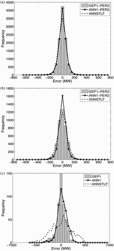
Fig. 6 ANN₁-ANN₂ and GEP₁-GEP₂ error distributions for the independent dataset: (a) weekdays and (b) weekends. Also shown are the errors from the operational ANNSTLF forecasts.

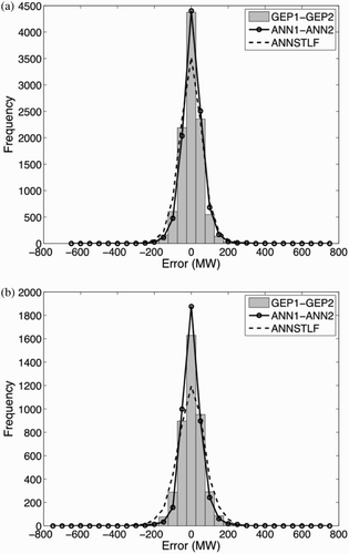
Figures 5a and 5b are very similar to Figs 6a and 6b, suggesting that any reasonable stage 2 (linear or non-linear) works well. GEP and ANN have nearly identical error distributions for weekdays, and both are better than ANNSTLF for this dataset. For weekends, ANN is best. For holidays, GEP is best.

Another way to compare the two-stage GEP, ANN and MLR with the operational ANNSTLF is to count how many days each method gave the best load forecast. These counts were divided by the total number of days in each category of weekdays, weekends, and holidays to give the relative counts in Fig. 7. ANN won for weekends and weekdays, while GEP won for holidays. The two-stage GEP and ANN gave the best forecasts much more often than the operational ANNSTLF.

Fig. 7 Proportion of time that any method was better than the others.

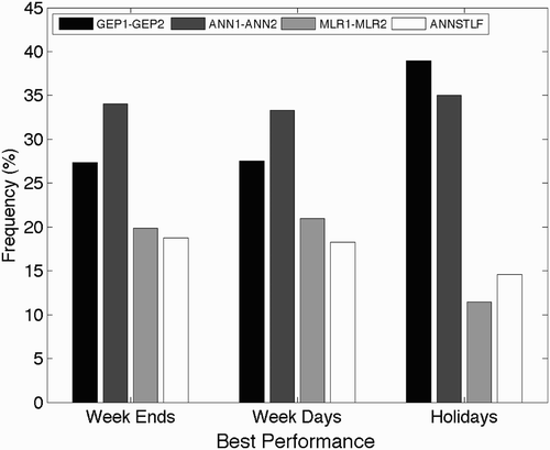
Both ANN and GEP gave excellent results for our dataset, when used as the first stage in a two-stage statistical scheme. For holidays GEP is slightly better, perhaps because it has less of an overfitting problem for small datasets compared to ANNs. For weekdays and weekends, ANN is better most often. The observation that each of those methods can be best for a substantial portion of days suggests that they could all be combined into an ensemble forecast—a topic for future research.

6 Multiple hour-ahead forecasts

The best fit statistical regressions from the one-hour-ahead forecasts can be applied iteratively to give forecasts more hours ahead. Namely, those equations gave L(t + 1) as a function of L(t), T(t), T(t + 1), etc. So once we have estimated the load at t + 1, we can apply that load to find the load at t + 2 (Khotanzad et al., 1998; Taylor and Buizza, 2002). For example, for GEP stage 1 L(t + 2) = GEP₁ [L(t + 1)), T(t + 1), T(t + 2), M(t + 2), D(t + 2), H(t + 2)] where T(t + 2) must be provided as a temperature forecast if used operationally or as ex post facto observations if used for perfect prog research at that valid time. The M, D and H variables are all calendar variables that are known in advance. Similar iterative equations can be made for the other statistical methods. Stage 2 can be applied similarly.

This process can be iterated more hours into the future. However, by using the forecast load rather than the observed load as input on the right-hand side of the equations, the errors will accumulate, and forecast quality will deteriorate with time. We demonstrated this using GEP₁-PER₂ and ANN₁-PER₂ forecasts, for which we calculated verification statistics from the independent dataset for forecast hours out to 24 h into the future. The result, in Fig. 8 using observed temperatures as input, shows that while forecast quality does indeed deteriorate with time into the future, the errors are nonetheless small enough to be useful to operational load forecasters.

Fig. 8 Increase in forecast error with lead time, for forecasts made by iteratively re-using the one-hour-ahead load forecasts with the observed temperatures for each hour. MAE is mean absolute error, and STD is standard deviation.

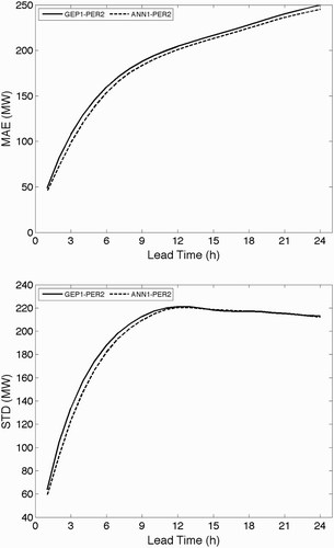
As an alternative experiment we applied the same two-stage method for a single, large, 24-hour time step. We found that the error for the single time step lead-time 24 h forecast was 2.1% of the total load, compared to the hourly iterative approach that gave an error of 3.5% of the total load.

7 Length of the training dataset

In this study we had the advantage of a long, seven-year dataset that we could split into training, testing and verification subsets. But how important was the length (5.25 years) of the training subset? Could an adequate forecast be made with just one year of training? Which statistical technique is more sensitive to a short training dataset?

To answer these questions, we re-ran GEP₁ and ANN₁ to find new best fit algorithms for stage 1 using a one-year training dataset (1 April 2008–31 March 2009). For stage 2 we used PER₂ based on that same one year of training data. We then verified GEP₁-PER₂ and ANN₁-PER₂ against the 1.75 years of independent data from 1 April 2009 to 31 December 2010 as used before. Table 2 shows the verification results for the one-hour-ahead forecasts.

The verification scores for the short (one-year) training were almost as good as those for the full five-year training period by applying a two-stage forecast. For both weekends and weekdays the short GEP is slightly better than the one trained over a longer time period (Table 3). This might be an artifact of the evolution procedure because the shorter dataset enables faster evolution, thereby testing a wider range of candidate functions during any given wall-clock time on the computer.

Table 3. Electric load forecast errors for the verification (scoring) dataset after the full two-stage regression but where either short or long datasets were used for training.

1 April 2009 to 31 December 2010, 1-hour Load Forecasts	ME (MW)	MAE (MW)	STD (MW)	r ^2
GEP1- PER2 Short
Weekdays	0.00	43	60	0.997
Weekends	−0.10	53	72	0.995
GEP1-PER2
Weekdays	0.02	44	61	0.997
Weekends	0.11	53	73	0.995
ANN1- PER2 Short
Weekdays	−0.06	49	67	0.996
Weekends	−0.18	52	71	0.995
ANN1-PER2
Weekdays	0.01	45	63	0.997
Weekends	−0.08	48	67	0.995

We were curious to see how stage 1 performed alone for the shorter dataset. The results are shown in Table 3. The artifact of the evolution period is clearly evident in the GEP data. Although it is clear that ANN had the smallest error for a single-stage load forecast with this short dataset, the performance of ANN with a short dataset was considerably worse than with a long one. As a result, GEP performed better than ANN in the second stage for weekdays.

8 Summary, discussion and conclusions

Using seven years of weather and electric load data for BC, Canada, we found that a two-stage (predictor-corrector) statistical process gave good and robust load forecasts. Non-linear statistical methods (gene expression programming (GEP) and artificial neural networks (ANN)) worked best for the first stage, and they captured most of the variance in the one-hour-ahead load signal. The remaining errors seemed to have a repeating pattern from one day to the next. This allowed the use of the error from 24 hours previously as a bias corrector in a second statistical stage to improve the forecast for the present hour. For this second stage, almost any non-linear or linear method (including 24-hour persistence) worked well. This two-stage method reduced the forecast mean absolute error to about 0.6% of the total electric load. The one-hour-ahead forecasts can be used iteratively to forecast more hours ahead, with the error increasing to about 3.5% of the total load after 24 hours of iteration.

To our surprise, the results from incorporating the day-before load as an additional predictor in stage 1 were not as good as the results from the two-stage method. This was true for both GEP and ANN, so this study focused on the two-stage method.

Using additional weather variables, such as dewpoint temperature, wind speed and weather conditions, did not add value to our one-hour-ahead forecasts (not shown here). However, it slightly improved the 24-hour lead time forecasts.

Both GEP and ANNs are commercially available as software packages (we used GeneXproTools by GepSoft and the ANN package in Matlab) that can run on desktop computers. GEP is a recent variant of genetic programming that evolves much faster and more efficiently. ANN has been proven by others to be able to fit almost any function but can have a problem with overfitting (i.e., fitting both the signal and the noise); this is less of a problem for GEP. This overfitting difficulty might explain why ANN had a problem fitting the load signal for holidays, which had a relatively small dataset.

The ANN gave the best load forecasts for weekends and weekdays in this case study. It had many more free parameters than GEP, yet GEP took longer (hours) to reach its best fit via evolution than it took ANN (minutes) to reach its best fit via back-propagation error minimization. Both methods yielded load algorithms that can be solved in seconds for any forecast hour. Future work will include combining load forecasts from GEP for holidays with ANN for weekends and weekdays with different lead-time nesting.

Acknowledgements

We are grateful for the funding we received from the Canadian Natural Sciences and Engineering Research Council (via Discovery and Strategic grants), the Canadian Foundation for Climate and Atmospheric Sciences, and BC Hydro. Heiki Walk and Doug McCollor of BC Hydro provided the load data and gave us valuable feedback.

Appendix: Illustration of a GEP algorithm

GEP devised the following algorithm for a single-stage, one-hour-ahead electric load forecast for weekdays, based on the long training dataset. The total stage-1 load is the sum of the loads from separate genes:

where the first gene is the dominant gene. The trigonometric functions treat their arguments as if the units were radians. All the input variables (M = month, T = temperature (°C), and H = hour) are for the valid forecast time (t + 1), except L which represents the previous-hour load L(t). The data points for GEP₁ in Fig. 2 were calculated using this algorithm.

Thus, even though GEP was allowed to use up to five genes, it used only four for this best solution. Also, GEP's solution did not include the previous-hour temperature T(t) or the day-of-week code D(t + 1), even though they were provided as input. The only operators used were +, −, *, /, ()², ()^1/3, exp, ln, sin, cos, and the other operators provided for this weekday were not needed for the stage-1 fit. Note that for weekends and holidays, GEP devised completely different stage-1 algorithms that look nothing like the equations above.

References

- Alfares , H. K. and Nazeeruddin , M. 2002 . Electric load forecasting: Literature survey and classification of methods . Int. J. Syst. Sci. , 33 : 23 – 34 .
- Amjady , N. 2007 . Short-term bus load forecasting of power systems by a new hybrid method . IEEE Trans. Power Syst. , 22 : 333 – 341 .
- Aytek , A. , Asce , M. and Alp , M. 2008 . An application of artificial intelligence for rainfall-runoff modeling . J. Earth Syst. Sci. , 117 : 145 – 155 .
- Bakhshaii , A. and Stull , R. 2009 . Deterministic ensemble forecasts using gene-expression programming . Weather Forecast , 24 : 1431 – 1451 .
- Bakhshaii , A. and Stull , R. 2011 . Gene-expression programming—an electrical-load forecast alternative to artificial neural networks. In: 91st American Meteorological Society Annual Meeting, 26–27 January 2011. Seattle, WA
- Bashir , Z. A. and El-Hawary , M. E. 2009 . Applying wavelets to short-term load forecasting using PSO-based neural networks . IEEE Trans. Power Syst. , 24 : 20 – 27 .
- Beccali , M. , Cellura , M. , Lo Brano , V. and Marvuglia , A. 2004 . Forecasting daily urban electric load profiles using artificial neural networks . Energy Convers. Manage. , 45 ( 18–19 ) : 2879 – 2900 .
- Chan , Z. S.H. , Ngan , H. W. , Rad , A. B. , David , A. K. and Kasabov , N. 2006 . Short-term ANN load forecasting from limited data using generalization learning strategies . Neurocomputing , 70 : 409 – 419 .
- Chen , B.-J. , Chang , M.-W. and Lin , C.-J. 2004 . Load forecasting using support vector machines: a study on EUNITE competition 2001 . IEEE Trans. Power Syst. , 19 : 1821 – 1830 .
- Cramer, N.L. 1985. A representation for the adaptive generation of simple sequential programs. In: Proceedings of the 1st International Conference on Genetic Algorithms, L. Erlbaum Associates Inc, pp. 183–187.
- da Silva , A. P.A. and Moulin , L. S. 2000 . Confidence intervals for neural network based short-term load forecasting . IEEE Trans. Power Syst. , 15 : 1191 – 1196 .
- Drezga , I. and Rahman , S. 1998 . Input variable selection for ANN-based short-term load forecasting . IEEE Trans. Power Syst. , 13 : 1238 – 1244 .
- EPRI (Electric Power Research Institute). 2009. ANNSTLF 5.2, Retrieved from http://www.dsipower.com/Software/EPRI-NSTLF/tabid/1880/Default.aspx
- Fan , S. and Chen , L. 2006 . Short-term load forecasting based on an adaptive hybrid method . IEEE Trans. Power Syst. , 21 : 392 – 401 .
- Ferreira , C. 2006 . Gene expression programming: Mathematical modelling by an artificial intelligence , 2 , Netherlands : Springer .
- Fildes , R. , Nikolopoulos , K. , Crone , S. F. and Syntetos , A. A. 2008 . Forecasting and operational research: a review . J. Oper. Res. Soc. , 59 ( 9 ) : 1150 – 1172 .
- Hinojosa , V. H. and Hoese , A. 2010 . Short-term load forecasting using fuzzy inductive reasoning and evolutionary algorithms . IEEE Trans. Power Syst. , 25 : 565 – 574 .
- Hippert , H. S. , Pedreira , C. E. and Souza , R. C. 2001 . Neural networks for short-term load forecasting: a review and evaluation . IEEE Trans. Power Syst. , 16 : 44 – 55 .
- Hippert , H. S. and Pedreira , C. E. 2004 . Estimating temperature profiles for short-term load forecasting: neural networks compared to linear models . IEE Proc-C , 151 : 543 – 547 .
- Holland , J. 1975 . Adaptation in natural and artificial systems , Ann Arbor : University of Michigan Press .
- Hsieh , W. W. 2009 . Machine learning methods in the environmental sciences: Neural networks and kernels , UK : Cambridge University Press .
- Huang , C. and Yang , H. 2001 . Evolving wavelet-based networks for short-term load forecasting . IEE Proc-C , 148 : 222 – 228 .
- Khotanzad , A. , Afkhami-Rohani , R. and Maratukulam , D. 1998 . ANNSTLF-artificial neural network short-term load forecaster generation three . IEEE Trans. Power Syst. , 13 : 1413 – 1422 .
- Koza , J. R. 1992 . Genetic programming: on the programming of computers by means of natural selection , Cambridge , MA : MIT Press .
- Liao , G.-C. and Tsao , T.-P. 2006 . Application of a fuzzy neural network combined with a chaos genetic algorithm and simulated annealing to short-term load forecasting . IEEE Trans. Evolut. Comput. , 10 : 330 – 340 .
- Ling , S. H. , Leung , F. H.F. , Lam , H. K. , Lee , Y.-S. and Tam , P. K.S. 2003 . A novel genetic-algorithm-based neural network for short-term load forecasting . IEEE Trans. Ind. Electron. , 50 : 793 – 799 .
- Mao , H. , Zeng , X.-J. , Leng , G. , Zhai , Y.-J. and Keane , J. A. 2009 . Short-term and midterm load forecasting using a bilevel optimization model . IEEE Trans. Power Syst. , 24 : 1080 – 1090 .
- Marin , F. J. , Garcia-Lagos , F. , Joya , G. and Sandoval , F. 2002 . Global model for short-term load forecasting using artificial neural networks . IEE Proc-C , 149 : 121 – 125 .
- Mori , H. and Yuihara , A. 2001 . Deterministic annealing clustering for ANN-based short-term load forecasting . IEEE Trans. Power Syst. , 16 : 545 – 551 .
- Musilek, P., E. Pelikan, T. Brabec, and M. Simunek. 2006. Recurrent neural network based gating for natural gas load prediction system. In: Proc. IEEE International Conference on Neural Networks, Vancouver, BC, Canada, 15–21 July 2006, art. no. 1716612, pp. 3736–3741.
- Osowski , S. and Siwek , K. 2002 . Regularisation of neural networks for improved load forecasting in the power system . IEE Proc-C , 149 : 340 – 344 .
- Roebber , P. J. 2010 . Seeking consensus: A new approach . Mon. Weather Rev. , 138 : 4402 – 4415 .
- Sadat Hosseini , S. and Gandomi , A. 2010 . Short-term load forecasting of power systems by gene expression programming . Neural Comput. Appl. , 21 : 377 – 389 .
- Srinivasan , D. , Tan , S. S. , Cheng , C. S. and Chan , E. K. 1999 . Parallel neural network-fuzzy expert system strategy for short-term load forecasting: system implementation and performance evaluation . IEEE Trans. Power Syst. , 14 : 1100 – 1106 .
- Stull , R. B. 2011 . Wet-bulb temperature from relative humidity and air temperature . J. App. Met. Clim. , 50 ( 11 ) : 2267 – 2269, . doi: http://dx.doi.org/10.1175/JAMC-D-11-0143.1
- Taylor , J. W. and Buizza , R. 2002 . Neural network load forecasting with weather ensemble predictions . IEEE Trans. Power Syst. , 17 : 626 – 632 .
- Yun , Z. , Quan , Z. , Caixin , S. , Shaolan , L. , Yuming , L. and Yang , S. 2008 . RBF neural network and ANFIS-based short-term load forecasting approach in real-time price environment . IEEE Trans. Power Syst. , 23 : 853 – 858 .