Comparing Winter and Summer Simulated Estuarine Circulations in Foxe Basin, Canada

Abstract

Foxe Basin is an Arctic inland sea located at the north of the Hudson Bay system (Canada). The characteristics of its estuarine circulation in winter differ from those in summer, mainly because of the sea-ice formation and cover. Using Lagrangian tracers and flux calculations from simulated data through a section at the outlet of the basin, we have shown that one-third of all the ice produced in winter is eventually exported toward the Labrador Sea. Foxe Basin is also a place where, in winter, latent heat polynyas to the west coexist with sensible heat polynyas around southwestern Foxe Peninsula, the latter resulting from an upwelling of intermediate water approximately 0.6°C above the freezing point of seawater. Sea ice affects circulation in the basin by adding friction at the surface layer and by shielding the sea surface from the atmosphere, which leads to an average reduction of 11% in the surface currents. Sea ice also extracts approximately 1.3 × 10¹⁴ kg of fresh water from the sea surface. Divided by Foxe Basin's surface area (0.2 × 10¹² m²) and by the freshwater density, this mass represents a mean layer of 0.65 m of fresh water. The salt transport anomaly versus depth at the outlet of the basin and the mean vertical buoyancy flux were also examined; this confirmed previous assumptions that the estuarine circulation forms a positive (summer)–negative (winter) couple. We suggest that the sensitivity of this couple to climate change may be used as a proxy to evaluate the impact of global warming in Foxe Basin.

RÉSUMÉ [Traduit par la rédaction] Le bassin de Foxe est une mer intérieure arctique située au nord du système de la baie d'Hudson (Canada). Les caractéristiques de sa circulation estuarienne en hiver diffèrent de celles de l’été, principalement à cause de la formation et de la couverture de glace de mer. Au moyen de traceurs lagrangiens et de calculs de flux basés sur des données simulées à travers une section à la sortie du bassin, nous avons montré que le tiers de toute la glace produite en hiver est éventuellement exporté vers la mer du Labrador. Le bassin de Foxe est aussi un endroit où, en hiver, des polynies de chaleur latente à l'ouest coexistent avec des polynies de chaleur sensible autour du sud-ouest de la péninsule de Foxe, ces dernières étant produites par des remontées d'eau intermédiaire dont la température est approximativement 0,6 °C au-dessus du point de congélation de l'eau de mer. La glace de mer influe sur la circulation dans le bassin en ajoutant du frottement dans la couche de surface et en faisant écran entre la surface de la mer et l'atmosphère, ce qui provoque une réduction de 11% dans les courants de surface. La glace de mer extrait aussi environ 1,3 × 10¹⁴ kg d'eau douce de la surface de la mer. Divisée par la superficie du bassin de Foxe (0,2 × 10¹² m²) et par la masse volumique de l'eau douce, cette masse représente une couche moyenne de 0,65 m d'eau douce. Nous avons aussi examiné l'anomalie de transport de sel en fonction de la profondeur à la sortie du bassin et le flux vertical moyen de flottabilité; cela a confirmé des hypothèses précédentes selon lesquelles la circulation estuarienne forme un couple positif (été) – négatif (hiver). Nous croyons que la sensibilité de ce couple au changement climatique peut servir d'indicateur pour évaluer l'impact du réchauffement planétaire dans le bassin de Foxe.

Keywords:

• estuarine dynamics
• ice circulation
• polynyas
• salt budget
• buoyancy fluxes
• positive-negative estuaries
• inland seas

1 Introduction

The estuarine circulation in Foxe Basin (FB), the northernmost of the three inland water bodies of the Hudson Bay system (HB; Figs 1a and 1b), exhibits quite different patterns in winter and summer. This study investigates its seasonal variability, mainly with the help of simulated data, because observations in this remote Arctic–subarctic region are scarce.

Fig. 1 Hudson Bay system (a) and Foxe Basin (b). In (a), the inset corresponds to Foxe Basin and its immediate neighbours. The model grid (partial, corresponding to the outputted data) is shown in (b); the star indicates the location of the mooring in Foxe Channel, the cross-section S is symbolized by the thick straight line, and the horizontal hatching shows the tidal flats area. The definitions of the acronyms are Baffin Bay (BB), Coats Island (CI), Foxe Basin (FB), Foxe Channel (FC), Fury and Hecla Strait (FHS), Foxe Peninsula (FP), Hall Beach (HaB), Hudson Bay (HB), Hudson Strait (HS), Lyon Inlet (LI), Melville Peninsula (MP), Mansel Islands (MI), Prince Charles Island (PCI), Repulse Bay (RB), Roes Welcome Sound (RWS) and Southampton Island (SI).

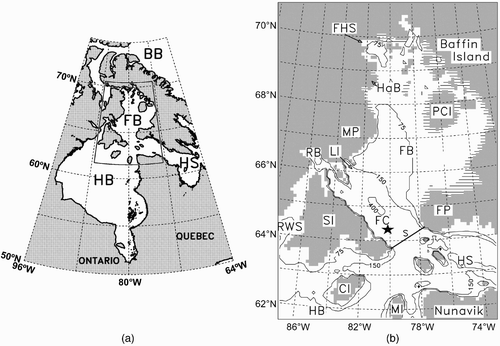
Physically, FB is a large and shallow sea, bordered to the north and northeast by Baffin Island (BI), to the west by Melville Peninsula (MP) and to the south by Southampton Island (SI). The mean and maximum depths are 90 and 450 m, respectively, and the surface area is about 0.2 × 10¹² m² (values from the National Oceanic and Atmospheric Administration's (NOAA's) 2-minute gridded global relief data (ETOPO2)). The basin receives Arctic water through Fury and Hecla Strait (FHS) and is connected to the Labrador Sea (LS) via Hudson Strait (HS).

The HB system plays an important hydrographic role by exporting fresh water toward the LS, although the throughflow of Arctic water toward the North Atlantic is small compared to the other passages of the Canadian Arctic Archipelago. On one hand, well-mixed Arctic water flows through FHS at 0.04 Sv (1 Sv = 10⁶ m³ s⁻¹) in winter, with a salinity of S = 32 (practical salinity scale used) and a temperature of T =  −1.7°C (Barber, 1965), while the throughflow is 0.1 Sv in summer, with S = 31 and T = 0.8°C (Sadler, 1982). By comparison, 2.0 Sv of seawater flows from Baffin Bay to the LS through Davis Strait (annual estimate; Melling et al., 2008). On the other hand, 29 mSv of oceanic fresh water, relative to a reference salinity S _ref = 34.8 (i.e., mean salinity of the Arctic Ocean) and 6 mSv of sea ice flow through HS (Saucier et al., 2004), while the corresponding estimated values through Davis Strait are 100 mSv of fresh water (with S _ref = 34.8) and 19 mSv of sea ice (Melling et al., 2008). Note that more recent annual transport estimates through Davis Strait (Curry et al., 2011) are very similar to those found by Melling et al. (2008) with 2.3 Sv of seawater, 105 mSv of fresh water and 11 mSv of ice. According to Drinkwater (1988), the net flow out of HS into the LS should be approximately 0.1 Sv, which corresponds to the net flow through FHS combined with the net freshwater input in the entire HB system. In other words, although 20 times (0.1 Sv versus 2 Sv) less seawater passes through the HB system than through Davis Strait, this ratio is only 3.4 (29 mSv + 6 mSv = 35 mSv versus 100 mSv + 19 mSv = 119 mSv) for the freshwater transport.

There is a large uncertainty range in the amount of fresh water flowing out of HS that depends greatly on the reference salinity. Straneo and Saucier (2008) estimated the freshwater outflow to be 78–88 mSv with S _ref = 34.8 and 28–29 mSv with S _ref = 33 (i.e., salinity of the inflowing water in HS). The first value (78–88 mSv) is higher than previous estimates based on net freshwater export (around 40 mSv; Drinkwater, 1988; Dickson et al., 2007). According to Straneo and Saucier (2008), this may be explained by water coming from Davis Strait, flowing in and then out of HS. However, the second value (29 mSv) is consistent with the estimate found by Saucier et al. (2004).

In winter, FB is almost completely covered by at least three kinds of sea ice: ice formed through thermodynamic growth and spread over the centre of the basin; brown ice mainly advected from the west, rich in trapped sediment, and accumulated over FB's eastern tidal flats; and ice formed through compaction of frazil ice in the polynyas of western FB, located at Hall Beach, along the eastern coast of MP and at Lyon Inlet. There is, however, no multi-year ice because the basin is generally ice free by the end of summer.

Using a numerical model, Saucier et al. (2004) have shown that the tides in FB are significant and clearly of semi-diurnal M₂ type (period 12.42 hours). Prinsenberg (1986a, 1986b) reports that the surface tidal currents observed in the HB system are reduced by about 20% in winter because of friction with the ice cover. Likewise, St-Laurent et al. (2008) found with both observations and simulations that the amplitude of M₂ in FB decreases in winter, which is likely caused by friction at the ice–ocean boundary. However, in this paper, the currents were averaged over each season (i.e., over many tidal cycles) in order to remove the contribution of the tidal currents.

Estuarine circulation can be positive or negative. Positive estuarine circulation occurs when a large horizontal density difference exists, leading to a pressure gradient, between fresh water at the surface coming from river runoff and oceanic salt water at depth (Pritchard, 1958; Hansen and Rattray, 1965). This pressure gradient induces a baroclinic circulation that is best seen by averaging over several tidal cycles. Other parameters such as precipitation, ice melting or surface warming can enhance the circulation by increasing the buoyancy flux, while wind or tidal-induced turbulence tend to reduce the strength of the circulation by breaking the stratification. There are two types of negative estuarine circulation (see El-Sabh et al. (1997) for a detailed description). The first type occurs in polar seas when freshwater removal at the surface caused by sea-ice formation during winter exceeds the freshwater input from runoff near the shores. The second type happens in arid conditions at lower latitudes, when evaporation exceeds runoff and precipitation.

The first type of negative estuarine circulation has been less studied (although some work has been done in the Arctic (El-Sabh et al., 1997; Macdonald, 2000; Carmack, 2007)), than the more accessible second type (e.g., Spencer Gulf and Gulf St. Vincent in southern Australia (Kämpf et al., 2009) and the Mediterranean Sea (Bryden et al., 1994)). This may change in the context of global warming because, in some polar seas, the circulation can be positive during summer and negative during winter, thus forming a positive–negative estuarine couple likely to be sensitive to climate changes (Macdonald, 2000).

The negative estuarine circulation in winter in FB belongs to the first type; it has been mentioned in the literature by Prinsenberg (1986a) but not quantified. The goal of this study is therefore to quantify the negative estuarine circulation in FB and see if it forms a positive–negative couple. The data came mainly from the numerical model developed by Saucier et al. (2004), and some observations are provided to allow comparisons. The model and method are described in Section 2. The seasonal features of the circulation, the mass transfers between FB and its surroundings, and the mean vertical buoyancy flux are detailed in Sections 3 and 4, respectively. Finally, the discussion and the conclusions are given in Section 5.

2 Model description and method

a Model

The numerical model developed and described in detail by Saucier et al. (2004) is based on the GF8 model of Stronach et al. (1993); it has been adapted and validated for the HB system. It is a z-level, hydrostatic, shallow water and incompressible formulation, with atmospheric (air temperature, winds, cloud cover and precipitation) and runoff (momentum, temperature and salinity) forcings.

The atmospheric forcings come from the Global Environmental Multiscale model (Canadian Meteorological Centre). The water levels are specified along the two open boundaries (FHS and the mouth of HS) and the initial conditions come from composite sets of observed and simulated data. Furthermore, the model is coupled to a dynamic and thermodynamic sea-ice and snow cover model.

Although the numerical grid covers the entire HB system, only the outputs corresponding to FB are used in this study. The simulated data include the seawater and sea-ice velocities, the seawater temperature and salinity, and the sea-ice growth rate and thickness. Several other physical quantities, such as the ocean–atmosphere heat fluxes, are also computed internally by the model but were not used here. The simulations cover the period from August 2001 to August 2005, but, except for the calculation of the mean salinity in Section 4.b, only the outputs corresponding to the winter and summer periods (22 October 2003 to 7 October 2004) defined in Section 3.a are used here.

The horizontal resolution of the grid is 10 km × 10 km, and its vertical resolution varies from 10 m at the surface to 30 m at the bottom of Foxe Channel (FC). The internal time step of the model is five minutes and the simulated data were averaged over a three-hour period. In order to estimate how appropriate the spatial resolution is, it is useful to calculate the internal Rossby radius (see Gill, 1982) which gives the scale of internal phenomena such as baroclinic adjustments. For an idealized two-layer ocean, this radius is:

where f is the Coriolis parameter, g is the gravitational acceleration, ρ₁, ρ₂ and h ₁, h ₂ are the upper (1) or lower (2) layer densities and depths, respectively. Here, ρ₁, ρ₂ and h ₁, h ₂ have been time-averaged over the period 2003–04. In the middle of FC (65°N latitude, 81°W longitude), f = 1.32 × 10⁻⁴ s⁻¹, ρ₁ = 1026.62 kg m⁻³, ρ₂ = 1028.64 kg m⁻³, h ₁ = 75 m and h ₂ = 450 m, which leads to r ≈ 8 km (8.6 km in winter and 8.3 km in summer). In the middle of FB (67°N latitude, 79.5°W longitude), f = 1.34 × 10⁻⁴ s⁻¹, ρ₁ = 1026.84 kg m⁻³, ρ₂ = 1027.13 kg m⁻³, h ₁ = 75 m and h ₂ = 125 m, which leads to r ≈ 3 km (2.8 km in winter and 2.6 km in summer). The model horizontal resolution is, therefore, greater than the internal Rossby radius and the small-scale processes that may occur in FB must be parameterized in order to be taken into account (the subgrid-scale horizontal mixing follows Smagorinsky's (1963) formulation for the viscosity, while a constant of 2.5 m² s⁻¹ is used for the scalar diffusivity). However, the horizontal resolution is sufficient for the calculation of mesoscale processes such as water, salt and ice transports.

b Method

In order to compare the summer and winter estuarine circulations in FB, it is convenient to average the three-dimensional (3-D) model outputs over each season. The two-dimensional (2-D; latitude–longitude) horizontal fields are obtained by time-averaging the surface and bottom model fields (see Section 3.c for a detailed explanation). There are two types of one-dimensional (1-D; depth) vertical profiles in this study: one for water and salt transport and one for temperature. For the transports, the profiles are obtained by time-averaging and summing over the length of section S defined at the outlet of the basin (Fig. 1b). This section, between the easternmost tip of SI and southwestern Foxe Peninsula (FP), is also a cross-section of FC, almost perpendicular to the channel's longitudinal axis. S is 114 km wide and the maximum depth along its length is 265 m. For the temperature, the profiles are obtained by time-averaging at the location of the mooring shown in Fig. 1b to allow comparison between the simulated data and the observations. This mooring was deployed from August 2004 to August 2005. It included temperature sensors (Minilog12, VEMCO-AMIRIX Systems Inc.) evenly spaced (12 m, except for the two sensors at 165 and 155 m depths) from a depth of 357 to 155 m.

In addition, Lagrangian tracers using the simulated sea-ice velocity field in FB are used in order to determine ice floe trajectories from the start of three significant periods: a) when the sea ice begins to form (in early November); b) in the middle of winter (early February); and c) when the sea ice starts to melt (early May). Note that the tracer exists as long as the ice thickness is greater than zero (i.e., as long as the sea ice has not completely melted at the tracer's location). Note also that when the ice floe runs aground, the tracer is simply terminated. These tracers are useful because they provide a time dependent picture of the sea-ice motion, whereas the calculation of ice transport through a section gives no information about the fate of the ice leaving FB.

3 Foxe Basin physical oceanography

a Winter and Summer Definition

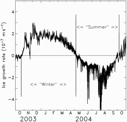
The oceanographic climate in FB can be conveniently defined using the rate of ice growth: a prolonged positive period corresponding to winter and, conversely, a prolonged negative period corresponding to summer. This definition of winter and summer based on the rate of ice growth is adequate in FB, because the surface circulation, as well as the dense water formation and circulation, depend strongly on the seasonal sea-ice formation and cover. In Fig. 2, the simulated rate of ice growth averaged over the entire domain of the basin shows that the 2003–04 year can be divided in two: the winter from 22 October 2003 to 5 May 2004 and the summer from 5 May 2004 to 7 October 2004. The start and end dates of these two seasons, plus or minus 15 days, are representative of the years 2001–05. In this study, all time-averaged calculations are, therefore, made over these two periods. These calculations include seawater, salt and sea-ice transport; seawater temperature, salinity and velocity fields; temperature profiles; rate of sea-ice growth, thickness and velocity fields. It is important to note that when the simulated data are seasonally averaged, the high frequency (e.g., tides) or transient (e.g., dense water pulses) phenomena are smoothed out. Note also that the averages may introduce apparent phase shifts as water masses formed during one season are included in the calculations of the following one but at different depths and/or locations.

Fig. 2 Simulated ice growth rate averaged over Foxe Basin. The positive (negative) values correspond to the formation (melting) of sea ice.

b Sea-Ice Dynamics

The sea-ice dynamics in FB affect the general circulation by adding friction with the underlying seawater, by shielding the sea surface from the atmosphere and by quickly exporting large amounts of frozen fresh water. The time-averaged sea-ice thermodynamic growth and velocity as well as the trajectory (Lagrangian tracers) of ice floes are detailed here in order to describe the ice dynamics in the basin.

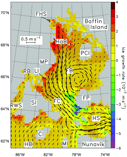
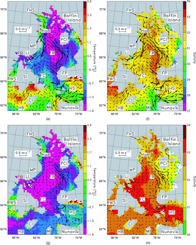
In Fig. 3, the ice growth field in FB clearly features three distinct areas: a high production rate zone of sea ice along the eastern coast of MP, with values exceeding 3.5 × 10⁻⁷ m s⁻¹, corresponding to the latent heat coastal polynyas in FB; a large central zone with production rates of about 1.5 × 10⁻⁷ m s⁻¹; and a small zone around the southwestern coast of FP with high negative production rates reaching –6 × 10⁻⁷ m s⁻¹. The first area has already been extensively described by Defossez et al. (2008, 2009) who found that high heat losses over the polynyas led to the formation of large amounts of frazil ice and dense water. The third area suggests that there is an upwelling providing sensible heat underneath the pack ice. The ice velocity field presents a distinctive “rack and pinion” pattern in FB: a significant ice current flows southward at the western side of the basin while a gyre around 180 km in diameter covers a large portion of the eastern part. This pattern is the result of the complex interactions between the ice motion, the cyclonic sea-surface currents, the strong northwesterly winter winds (with peaks close to 20 m s⁻¹; Defossez et al. (2009)) and the enclosed topography. The relatively high values of the ice velocity field in FB (0.25 ± 0.09 m s⁻¹, averaged over the whole basin) contrasts with the weaker ice current seen in northern HB (0.11 ± 0.09 m s⁻¹, averaged over the northern part of the bay). Figure 3 also shows that there is continuity between the ice currents in FB and HS, although this is more obvious for the ice flowing around the south of the three small islands at the head of HS than through the upwelling zone at the south of FP, suggesting that most of the sea ice exported by the basin subsequently enters the strait.

Fig. 3 Simulated ice growth rate averaged over the winter in Foxe Basin. The positive (negative) values correspond to the formation (melting) of sea ice. The vector field corresponds to the sea-ice velocity; its scale is given in the upper left box (see Fig. 1 for acronym definitions).

Because section S is located at the mouth of FB (Fig. 1b) and corresponds to the main strait between the basin and the other parts of the HB system, ten Lagrangian tracers (T₁ to T₁₀) were evenly spaced along its width and released in order to determine the fate of the sea ice leaving FB. This procedure was repeated at the start of three significant periods (beginning, middle and end of winter). The trajectories of the tracers are shown in Fig. 4. In addition, the mean speed and total distance covered by each tracer is reported in Table 1.

Fig. 4 Simulated sea-ice trajectory in Foxe Basin. The colour code of the tracers corresponding to the trajectories is given in the upper left box. In panels (a), (b) and (c), the run starts 1 November 2003, 1 February 2004 and 1 May 2004, respectively (see Fig. 1 for acronym definitions).

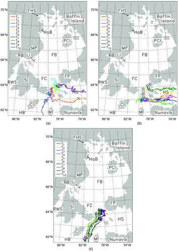
Table 1. Mean speed and total distance covered by the Lagrangian tracers leaving Foxe Basin (see Fig. 4 for trajectories). The dates indicate the start of each run (beginning of ice formation, maximum ice formation and beginning of ice melting). The last line contains the averaged speed for all tracers along with the standard deviation.

Tracer No.	1 November 2003		1 February 2004		1 May 2004
	Mean Speed (m s^−1)	Total Distance (km)	Mean Speed (m s^−1)	Total Distance (km)	Mean Speed (m s^−1)	Total Distance (km)
T1	0.18	17	0.01	0	0.02	0
T2	0.14	233	0.16	2428	0.13	994
T3	0.19	837	0.19	2586	0.15	1168
T4	0.26	1135	0.21	1353	0.16	1237
T5	0.32	1465	0.23	1218	0.17	1283
T6	0.40	1601	0.11	389	0.18	1367
T7	0.29	180	0.20	320	0.19	1340
T8	0.15	79	0.27	1404	0.20	1379
T9	0.11	95	0.16	89	0.21	1349
T10	0.19	935	0.13	87	0.25	759
Speed (m s^−1)	0.22 ± 0.10		0.17 ± 0.08		0.17 ± 0.07

At the beginning of the ice formation period (1 November 2003; Fig. 4a), most of the tracers exit FB and flow toward HS although their trajectories can temporarily return to the basin (e.g., T₅ and T₆). The island complex at the head of HS clearly separates the ice flow into a direct route south of FP and a longer one bypassing the islands to the south. By taking the longest route the speed of the tracers entering HS (e.g., approximately 0.3 m s⁻¹ for T₄ and T₅) is a bit faster than the others (e.g., 0.19 m s⁻¹ for T₁₀). This may be a result of the surface current system in HS, with currents flowing westward in the northern part of the strait (along the southern coast of BI) and eastward in the southern part (along the northern coast of Nunavik). Note that HS is only sparsely covered by sea ice during this period.

The situation changes appreciably in the middle of winter (1 February 2004; Fig. 4b) because all tracers enter HS with smoother and more direct trajectories. Furthermore, the speed of the tracers close to the south of FP seems generally higher than the speed of the tracers close to the eastern tip of SI (from 0.16 m s⁻¹ for T₂ to 0.27 m s⁻¹ for T₈). This can be explained by the north to south cross-channel flow in HS (Drinkwater, 1988) that tends to pile the ice on the southern coast of the strait, leaving a lower ice concentration on the northern side where the sea ice advected from FB can travel faster. Therefore, although the overall surface currents are reduced by friction with the ice cover, there exists a dichotomy between the northern and southern sides of the strait, leading to a difference in ice velocity in both parts.

The situation changes again at the beginning of the ice melting period (1 May 2004; Fig. 4c) since all tracers now penetrate deeply into northeastern HB. They do not, however, flow much below the 62°N parallel at which point they perform a “U-turn” toward HS. It is possible that the strong coastal current flowing along eastern HB toward HS (Saucier et al., 2004) drives this ice. Here also, the speed of the tracers close to FP is greater than the speed of the tracers close to SI (from 0.13 m s⁻¹ for T₂ to 0.25 m s⁻¹ for T₁₀). Note that all the tracer trajectories end because the ice to which they were attached has melted. Finally, the melted ice seems to flow toward HS; this indicates that the ice (solid or melted) coming from FB and entering HB eventually leaves the bay and subsequently enters HS.

c Water Characteristics and Mean Circulation

The mean circulation in FB is cyclonic in all seasons (Prinsenberg, 1986a; Saucier et al., 2004), as shown in Fig. 5. However, because of the topography (see Fig. 1b), only the surface currents are truly cyclonic. All the water below the break at 150 m depth between FC and the large northern part of FB flows more or less along the channel's longitudinal axis.

Fig. 5 Simulated temperature (panels (a), (c), (e), (g)), salinity (panels (b), (d), (f), (h)) and seawater velocity fields (panels (a)–(h)), averaged over winter and summer in Foxe Basin. The velocity scale is given in the upper left box. (a) and (b) correspond to the winter surface fields; (c) and (d) to the winter bottom fields; (e) and (f) to the summer surface fields; and (g) and (h) to the summer bottom fields. In order to ease the reading of the figures, the velocity field is the same in (a) and (b), (c) and (d), (e) and (f), and (g) and (h). Note that, in (c), (d), (g) and (h), the fields are, in fact, calculated near the bottom because they correspond to the middle of the deepest grid cells (see Fig. 1 for acronym definitions).

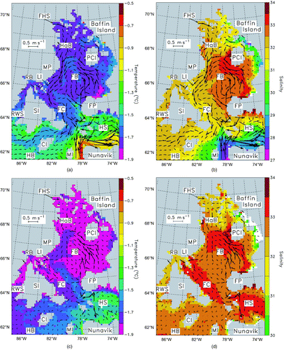
Fig. 5 Concluded

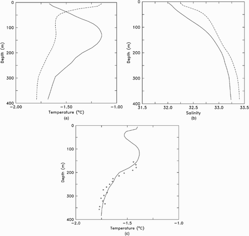
Figure 6a indicates that the thermocline in central FC is around 100 m in winter and 50 m in summer. This is deeper than most of the northern part of FB, composed mainly of shallow water and tidal flats. The warm core that can be seen in winter is likely the result of an intrusion of intermediate water, because the location of the mooring (Fig. 1b) is close to HB and HS. Figure 6b shows that there is no strong halocline in either season. The comparison (Fig. 6c) between the simulated and observed temperatures at the location of the mooring indicates that the simulation is in good agreement with the observations, for the depths where the latter are available. Note that the start and end (August 2004 and August 2005, respectively) of the time series do not correspond to the summer and winter periods defined in this study, and the simulated data in Fig. 6c were averaged over the period of the time series.

Fig. 6 Simulated temperature (a) and salinity (b) and the comparison between simulated and observed temperature (c) profiles versus depth in Foxe Channel. The location of the profiles corresponds to the mooring deployed at 64.37°N and 80.55°W from August 2004 to August 2005 (see Fig. 1b). In (a) and (b), the solid and dashed lines represent the winter and summer, respectively. In (c), the circles correspond to the observations and the solid line to the simulated data averaged over the period matching the time series.

Furthermore, Figs 6a and 6b show that, when averaged over each season, there is no mixed layer in the channel (the first level of the grid model is 10 m deep and cannot properly represent shallower layers). It is, therefore, not possible to define a fixed surface layer height greater than the first grid level depth over which the seawater properties could be integrated because this would lead to a bias for a large part of the basin. A similar argument could be applied to the bottom of the basin because only the bottom of FC would then actually be taken into account if a fixed bottom layer height was used. In particular, this could not properly represent the dense water originating from the western polynyas of FB, flowing along MP and cascading into FC. This is why in this study, in order to consider the water characteristics at the scale of the entire basin and to preserve the continuity of the water masses, the seawater characteristics and circulation were examined at the sea surface and near the bottom of the basin.

At the surface, the calculations were made on the first level of the numerical grid, so that the thickness is equal to 10 m and the depth to 5 m (= 10/2). Near the bottom, the calculations were made on the last level of the numerical grid; in that case, the thickness and depth depend on the bathymetry, so that the layer is at most 30 m thick and the depth is, on average, 35 m (= 20 + 30/2; 20 m being a mean value taking into account the irregularities of the sea bottom) above the bottom in the deepest parts and much less (minimum 5 m) in the shallowest parts. Although the bulk circulation is not explicitly described here, it will be implicitly treated in Section 4 with the calculation of mass transports through section S.

1 In winter

i At the surface

The surface velocity field (Fig. 5a or 5b) in winter is globally cyclonic in FB. The current distribution is relatively homogeneous (weaker currents at the centre of the basin and stronger currents at its periphery) in the region defined by 64°–68°N latitude and 74°–83°W longitude. More precisely, the winter surface current averaged over the entire domain of FB is 0.35 ± 0.09 m s⁻¹, and the difference between the surface currents averaged from 66° to 68°N and those averaged from 64° to 66°N is only approximately 3%. In the vicinity of section S (Fig. 1b), Fig. 5a or 5b shows that the current tends to exit the basin.

The sea surface temperature (SST; Fig. 5a) is close to the freezing point (T_f  = −1.85°C) because of air temperatures frequently below −30°C in winter over FB. A notable exception can be seen around southwestern FP where there is surface water at T = −1.3°C. The surface current field shows that this is not an intrusion of surface water from HS despite the apparent continuity in temperature because, in this area, the current points southeastward. This warmer zone corresponds well to the suspected upwelling region described in Section 3b and may originate from HB and/or HS intermediate water. No surface water from HB crosses into FC. Instead, it flows along the coast of Nunavik and enters HS, supplying the latter with water around −0.8°C. On the contrary, cold surface water from FB bypasses the east of SI and penetrates deep into the north of HB.

The sea surface salinity (SSS; Fig. 5b) presents a more varied picture with a continuously positive gradient from the southwest (S ≈ 31.5) to the northeast of FB (S ≈ 33.5), with the exception of a large zone (where S < 30) fed by three rivers on BI in the northeast of the basin. This gradient is related to the bathymetry because the highest salinity zone (S > 33) corresponds to the tidal flats where brine rich seawater is repetitively exposed to very cold air temperatures during ebb tide (Campbell, 1964). The SSS around southwestern FP is higher on the FB side (S = 32.5) than on the HS side (S = 32), thus confirming that the surface water of the strait does not enter the basin. The distribution of salinity is also consistent with that of temperature because it shows that no surface water from HB enters FB (it clearly flows into HS instead, with a low salinity around 28.5) and that surface water (S = 32) of southern FB penetrates deep into the north of the bay.

Because it was suggested that there is an upwelling region around southwestern FP, it would be interesting to check the simulated vertical component w. The mean winter value of w averaged over the whole volume of FB is (the minus indicates the downward direction), while w averaged over the area under the negative ice growth rate zone described in Section 3.b (see also Fig. 3) is . The difference between the two mean vertical speeds is sufficiently high to prove, with the model data, the existence of an upwelling of water at T ≈ −1.3°C and S ≈ 32.5. The origin of this upwelled water is not easy to determine because water masses from FB, HS and HB collide in this area. At a depth of 150 m and 100 km from the southernmost tip of FP, the temperature and salinity are around −1.6°C and 32.7 in FB, while they are −0.7°C and 32.5 in HS and HB. When the upwelled water reaches the surface, it is cooled by the very cold air temperature, so it is possible that this water comes from HS or HB intermediate water. Tracer experiments would be useful to determine the origin of the upwelling around FP precisely, but this is beyond the scope of this study. One can hypothesize that the accumulation of deep water against the topographic constriction made by the three small islands near the head of HS forces any lighter incoming intermediate water mass to flow over it.

ii Near the bottom

The bottom velocity field (Fig. 5c or 5d) is given here mainly for information because the depth in FB varies from 5 to 450 m. As can be expected, the field is nearly identical to the surface field over the shallower parts of FB. Also, the mean velocity near the bottom of FC is 0.12 ± 0.05 m s⁻¹ (i.e., three times less than at the surface). Note that this averaged value does not accurately describe the deep circulation in the channel because it smoothed out the dense water pulse that renews two-thirds of the deep water in FC (Defossez et al., 2008).

The sea bottom temperature in winter (SBT; Fig. 5c) shows the trail of a large intrusion of intermediate water at around −1.6°C from HB and/or HS, flowing along the northern side of FC. The bottom of this intrusion varies from 100 to 200 m depth. Although most of the bottom of FB is near freezing, it is interesting to note that in areas like the shallow channel along MP, any dense water has been flushed away by slightly warmer currents.

The sea bottom salinity (SBS; Fig. 5d) also shows some continuity between the intermediate HB and HS waters and the intrusion in FC because S ≈ 32.5 on both sides. Furthermore, the SBS indicates that the deep water in FC is efficiently blocked by the sills and topographical constrictions between SI and the head of HS. The large high salinity area (S > 33) in northern FB corresponds to saline water ponds repeatedly exposed to very cold air temperatures over the tidal flats.

2 In summer

i At the surface

The surface velocity field (Fig. 5e or 5f) in summer is still globally cyclonic in FB with a mean value of 0.39 ± 0.08 m s⁻¹ (i.e., approximately 11% higher than in winter). Furthermore, in the region defined by 64°–68°N latitude and 74°–83°W longitude, the surface currents, averaged from 66° to 68°N, are now approximately 26% stronger than those averaged from 64° to 66°N (in winter this was 3%). This suggests that the sea-ice motion and friction with the surface water has a smoothing effect on the circulation in winter. This also indicates that the ice cover efficiently shields the sea surface from the rapidly changing momentum transfer of the winds, despite the fact that a 21-year near-climatology has shown that, over FB, the winds are significantly stronger in winter than in summer (Defossez et al., 2009).

Over FB, the SST (Fig. 5e) is much less homogeneous than in winter; in particular, there is a large, central area of near-freezing water which is likely a remnant of the preceding winter surface water and of drifting ice. This area is located over the shallow part of FB and does not encroach upon FC. The warmer (T > 0°C) parts of the basin correspond to the mouths of FHS and the rivers on BI. Furthermore, surface water around 0°C in northern HB, seemingly joined by some HS surface water, bypasses the eastern coast of SI and enters FB. This intrusion of surface water also prevents the cold central area in FB from spreading over FC. The opposite situation prevailed in winter because it was FB surface water that entered the north of the bay.

The SSS (Fig. 5f) in FB matches the general picture obtained with the SST in summer. It shows that the large central area is saltier (S = 32.5 versus 31.5) than the rest of the basin and that the fresher parts (S < 31) also correspond to the mouths of FHS and the rivers on BI. The small patch of salty water (S = 32.5) at the southwestern tip of FP may be an indication that the upwelling in this region is still active because the mean summer value of w is . Note that this upwelling could not be seen with SST alone because the temperatures in this area and its surroundings are very close (T ≈ –1.3°C). Lastly, Fig. 5f tends to confirm the intrusion of surface water (S ≈ 31) from HB and/or HS seen in the previous paragraph with the SST, although a water mass of similar salinity exists in the basin, making it difficult to distinguish them from each other. This indicates that although FB exports surface water all year long (the mean outflow from FB is always positive, as will be shown in Section 4.b), external surface water intermittently enters the basin.

ii Near the bottom

The summertime bottom velocity field (Fig. 5g or 5h) in FB is very similar to that in winter. This similarity suggests that the ice cover has little effect on the mean circulation at depth in FC. Also, it is important to remember that it is the freshwater and salt fluxes that actually define the type of estuarine circulation, not the current pattern. The SBT in summer (Fig. 5g) bears the mark of the preceding winter in most of the FB area, and especially in the deepest parts, such as FC which is filled with freezing water, the exceptions being the mouths of FHS and the rivers on BI (T > 0.5°C). There still seems to be an intrusion of intermediate water at −1°C, coming from HB and/or HS that flows around southwestern FP. There is also some freezing water in northern HB which corresponds to the wake of the intrusion of surface water from FB formed during the preceding winter, although neither in situ production in the northwestern polynyas of HB nor the remnant of an overflow of deep water from FC can be ruled out.

The SBS (Fig. 5h) confirms the results obtained with the SBT: the deepest parts of FB are filled with very saline water (S > 33), and low salinity water exits the mouths of FHS (S < 31.5) and the rivers on BI (S < 30). The continuity between the deep water of FC (S = 33.5) and HS is only apparent because the temperature (Fig. 5g) shows that, in reality, they are different (T = −1.9°C in FC versus –0.5°C in HS). Lastly, the presence of very saline water coming from FC, beyond the sill between SI and the head of HS, flowing into HB suggests that this is the remnant of an overflow.

4 Mass transfer between the surrounding parts of Foxe Basin

a Ice transport

The total amount of sea ice leaving the system during a given period can be estimated by integrating the flow of ice through section S (Fig. 1b) at the outlet of the basin. The flow is the sum of the products of the ice thickness (Fig. 7) by the ice velocity and by the length of the grid cells along S. Although the summer was defined in this study as the period during which the ice growth rate averaged over FB was negative, it must be included in this calculation because the basin is generally only ice free by the end of September. The simulated data for the period 22 October 2003 to 7 October 2004 give a total of 1.3 × 10¹⁴ kg of ice passing through section S. It is interesting to compare this value with the total amount of sea ice produced in the basin, 4.2 × 10¹⁴ kg, which is obtained by integrating the ice growth rate in Fig. 3 over the winter. Therefore, almost one-third (1.3 × 10¹⁴/4.2 × 10¹⁴) of all the ice produced in FB leaves the system and eventually flows, as sea ice or melted ice, toward the LS. In terms of freshwater transport, the amount of exported ice corresponds to a mean annual value of 4 mSv.

Fig. 7 Simulated sea-ice thickness averaged over the winter in Foxe Basin (see Fig. 1 for acronym definitions and Fig. 3 for the vector field description).

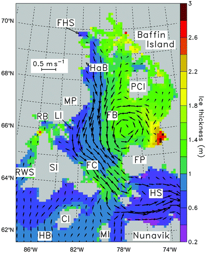
In Fig. 7, the ice thickness is appreciably greater to the east of FB than to the west. The distributions of the ice velocity and ice thickness fields are closely related, especially on the western side of the basin where stronger ice currents correspond to thinner ice. When the ice growth rate (taken from Fig. 3) is integrated over the winter and over the area (2 × 10⁹ m²) north of FP where the ice thickness reaches values up to 3 m locally, the resulting mean thickness is 1.9 m, while it is 2.5 m when the ice thickness (taken from Fig. 7) is averaged over the same period and area. The 0.6 m difference in thickness shows that sea ice is advected toward eastern FB and accumulates there (note that the model resolution is not high enough to represent small-scale phenomena, such as ice ridging, accurately). It is also interesting that the sea ice tends to accumulate at the outlet of FB because of the complex formed by the three small islands at the head of HS.

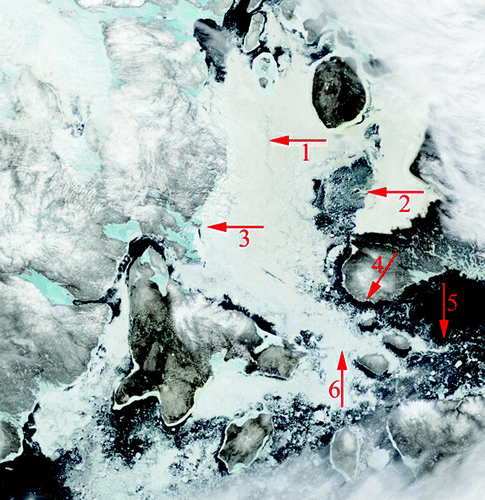
Most of these sea ice results can be seen on the satellite image in Fig. 8. In particular, arrow 1 points to the demarcation line between the southward ice current on the western side of the basin and the gyre at the eastern side; arrow 2 shows that the shear stress induced by the gyre tends to break the pack ice; arrow 3 pinpoints the location of the western latent heat polynyas in FC at Lyon Inlet; arrow 4 shows that the ice-free area below FP is compatible with the presence of sensible heat polynyas; arrow 5 highlights the fact that the ice floes tend to pass to the south of the three small islands at the head of HS and rejoin the southern circulation in the strait; finally, arrow 6 points to the area of accumulation of sea ice at the head of HS. Note that the satellite image was taken in 2002, but it is assumed here that the large-scale features of ice distribution and dynamics are comparable to those features in 2004, although they may differ quantitatively. Therefore, the model reproduces the observed ice circulation well. This was, in fact, expected because the coupled sea-ice model was validated (Saucier et al., 2004) by checking the good agreement between the simulated data (sea-ice concentration and thickness) and observations from the Canadian Ice Service of the Meteorological Service of Canada.

Fig. 8 Satellite image taken 20 June 2002 over Foxe Basin and its surrounding parts (copyright NASA, 2008). The significance of the arrows is given in Section 4.a.

b Seawater and Salt Transport

When characterizing the estuarine circulation, it is useful to draw the vertical profile of the water flow, averaged over a long period (greater than several months so that the spring and neap tide cycles are also filtered out) in order to remove tidal movements, as well as transient wind bursts, through a section as perpendicular as possible to the main direction of the current. This indicates immediately if the surface, intermediate and deep waters flow into or out of the estuarine system. This must be completed, however, by the vertical profile of the salt flow through the same section in order to determine the salt balance and whether or not the system type is positive or negative. At high latitudes, this approach is more pertinent in winter than in summer, because the sea ice reduces the wind and tidal contributions by shielding the sea from the atmosphere and by adding friction at the sea surface.

It is important to note that the processes leading to a positive or negative estuarine circulation are quite different. In a positive estuarine system, the freshwater inflow is mainly from river runoff (by assuming that precipitation balances evaporation), the saltwater inflow is from an intrusion of sea water at depth, and the outflow is a mixture of the fresh water and saltwater. All these flows can be considered “horizontal.” Conversely, in a negative estuarine system, the freshwater outflow caused by evaporation or ice formation is “vertical,” implying that fresh water is permanently removed from the system, rather than being mixed with saltwater. However, the saltwater outflow, which takes the form of a current of dense water, and the intermediate water inflow are still “horizontal.”

For an idealized positive–negative couple (i.e., when the wind and tidal contributions can be neglected), the previous remark can be shown as follows:

This means that when an estuarine system is positive (negative), it adds (extracts) fresh water at the surface and saltier water at depth and exports (imports) a mixture of the two as intermediate water. Globally, the estuarine circulation keeps the balance between these water masses. Thus, for a positive–negative couple, the salt transport anomaly versus the depth profile should be “X–shaped,” so that the backslash (\) and forward slash (/) parts correspond to the positive and negative estuarine circulations, respectively.

The vertical water flow profile is shown in Fig. 9a where the flow is summed by layers 10 m thick from the surface to the bottom, over the length of section S (Fig. 1b) and averaged over winter and summer 2004. It can be seen that, in both seasons, FB exports surface and bottom waters while there is a significant intrusion of intermediate water (between the depths of 80 and 210 m in winter and 40 and 190 m in summer). This intrusion was described in Sections 3.c.1.ii and 3.c.2.ii. Interestingly, the profile shows that the basin exports more surface water than bottom water in winter, while the opposite situation prevails in summer when the mean surface summer velocity is 11% higher (see Section 3.c.2.i). This indicates that although the ice cover alters the circulation, it seems to have little effect on the overall intensity of the exchanges between the basin and its surroundings.

Fig. 9 Vertical simulated seawater (a) and salt (b) transport through cross-section S in Foxe Channel (see Fig. 1b). The solid and dashed lines correspond to the winter and summer, respectively. In (a) and (b), the transport is calculated through 10 m thick layers on S from the surface to the bottom of the channel. In (a), negative (positive) values indicate an output (input) stream; in (b), the salt transport anomaly is defined as the difference between the salinity measured at the section and the mean salinity in Foxe Basin.

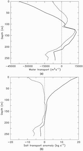
The net transport of seawater through section S (not counting the ice) corresponds to the sum over the depth of the flow profile in Fig. 9a. It is 0.09 Sv in winter and 0.013 Sv in summer; this gives a mean annual value of 0.056 Sv. This mean value was weighted according to the duration of the winter and summer (196 and 155 days, respectively). The same result was obtained if the calculation was done for each model time step from 22 October 2003 to 7 October 2004. It is useful to estimate the amount of surface water flowing between FB and HB (HS excluded) by calculating the transport for z < 80 m. In winter, the outflow from FB to HB is 0.15 Sv, and in summer the inflow from HB to FB is 0.01 Sv. This shows that the great difference between the net transport in winter and summer is essentially a result of the inversion of the surface water flow between FB and HB and not to an increase in river runoff or transport through FHS since they are both significantly reduced in winter.

In order to draw the vertical salt profile (Fig. 9b), it is necessary to determine first the mean salinity in FB because this profile is defined by the following product:

where is the salt transport anomaly through section S (function of the depth: index j), is the seawater volume transport through S (function of the width of S: index i, of the depth: index j, and of the time: time step Δt), is the salinity of the section (same dependencies as ), and S _mean ≈ 32.67 is the mean salinity of the entire basin averaged from August 2001 to August 2005. Note that in Eq. (2), the salinities are expressed in kg m⁻³. Note also that in Eq. (2), the diffusion is neglected. A comparison between the contributions to the transport of the diffusion term K_h ∇∇ _hS · n (K_h  = 2.5 m² s⁻¹ being the horizontal diffusivity, S the salinity and n the unit vector normal to the section) and the advection term S v _h  · n (v _h being the horizontal velocity of the current) indicates that, in the vicinity of section S, the advection is generally more than three orders of magnitude greater than the diffusion for most of the year. The winter profile shows a typical negative estuarine circulation because there is more fresh water extracted at the surface by ice formation and export than is brought in by runoff or precipitation, and more salt is extracted by brine enrichment of the deep water and export with the bottom currents. In summer, although fresh water is added to the surface, the profile does not fit the pattern of an ideal positive estuarine circulation exactly because a significant amount of salt is removed at the bottom. This is a consequence of the dense water pulse originating from the latent heat polynyas in western FB in February that takes six months to cover the distance (310 km at 2 cm s⁻¹) separating Lyon Inlet (Fig. 1b) from the section. The dense water pulse, lasting about three months, is superimposed on the estuarine circulation in summer, and this explains why the profile in Fig. 9b is not quite “X–shaped.” Figure 9b also shows that for both seasons, the salt balance for the intermediate water is almost neutral.

To summarize, FB presents the characteristics of a positive–negative estuarine system, although the dense water propagation at depth in FC affects the estuarine circulation in summer. However, it is possible that neglecting the wind and tidal contributions is an oversimplification, which would explain some of the deviations from the idealized case in Fig. 9. Yet it is also important to note that a positive–negative couple such as in FB is always in a transient state, which makes techniques developed for steady positive or negative estuarine systems inappropriate.

c Vertical Buoyancy Flux

Although the seawater and salt transport give useful information about the circulation in general, this is not sufficient to fully characterize the estuarine circulation, because the circulation may include contributions from the winds and the tides (Nihoul and Ronday, 1975). However, it is difficult to separate the different components of the circulation, because their importance may vary greatly from one location in FB to another; this would require a fine resolution that the model does not provide. One way to circumvent this problem is to consider the vertical buoyancy flux, because it is the most important process affecting the dynamics of all types of estuaries (Geyer et al., 2008), and to average it over the whole domain.

Most of the time the temperature minima and maxima in FB are less than 1°C apart (see Fig. 5), the buoyancy flux in the basin is, therefore, mainly a result of variations in salinity and can be expressed using Geyer et al.’s (2008) formulation:

where, β = ∂ρ/ρ∂s, s′ and w′ are the turbulent components of the salinity and vertical velocity, respectively. Note that Eq. (3) might be inaccurate in the latent heat polynyas located in western FB, because strong convection resulting from the formation of ice occurs there, which leads to the sinking of cold and salty water. However, the combined surface area of these polynyas is smaller than the rest of the basin by two orders of magnitude, and Eq. (3) is likely to remain valid at the scale of the basin. The flux is averaged on all the grid nodes in FB, and the resulting mean vertical buoyancy flux is drawn in Fig. 10.

Fig. 10 Mean vertical buoyancy flux in Foxe Basin (see Section 3.a and Fig. 2 for the winter and summer definitions).

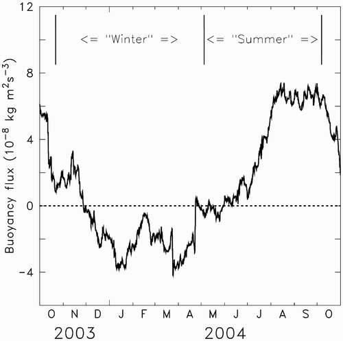
Figure 10 shows clearly that the buoyancy flux follows the seasonal cycle: it is negative in winter and positive in summer, thus confirming that the circulation in FB has the characteristics of a positive–negative estuarine system. The negative buoyancy flux period starts approximately 40 days after the beginning of winter and lasts 147 days. The transition between the positive and negative parts of the curve is smooth at the end of summer (28 November 2003) and abrupt at the end of winter (23 April 2004), as if the ice pack was holding back the negative flux until the thaw. From 23 April to 11 June, the mean flux is around zero, suggesting either that positive and negative estuarine circulations coexist in the basin for 49 days and that they compensate each other or that the estuarine circulation is turned off during this period.

The positive buoyancy flux period also starts approximately 40 days after the beginning of summer and lasts 170 days (i.e., almost one month longer than the negative flux period). The amplitude of the positive buoyancy flux is twice the negative one, showing that the positive–negative couple in FB is asymmetric. It is interesting to note that in midwinter (i.e., around 15 February 2003) the negative flux is near zero, while during the same period the air temperature and winds over FB are at their extreme. Because this corresponds to the opening of the western polynyas along MP in FB, it confirms that they do not play a large role in the overall estuarine circulation. Thus, the model suggests that above a certain threshold, the sea ice shields the sea surface from the atmosphere very effectively, leading to a temporary halt of the estuarine circulation.

5 Summary and conclusions

The FB seasonal cycle is dominated by sea-ice processes, so the winter and summer seasons are well defined by the ice-growth rate. The dynamics are affected by friction and shielding by the sea-ice cover. Ice growth is significant in winter, with the largest production associated with the latent heat polynyas in western FB, while ice tends to accumulate in the eastern part of the basin. The model indicates that there is an upwelling of water 0.6°C above the freezing point (T_f  = −1.85°C) to the surface in southwestern FP; this is compatible with the observation of polynyas, leads and cracks in this region (Laidler and Elee, 2008).

The mean circulation in FB is cyclonic in winter and summer, and the mean surface velocity field is slightly less than 0.4 m s⁻¹ in both seasons. The influence of very low air temperatures in winter is clearly seen in the SST because the entire domain is around the freezing point. These low temperatures propagate to the bottom, and a significant amount of cold water survives until the next winter, especially in the central and deep parts of the basin. The salinity presents a contrasting picture with brine-rich water (S > 33.5) over the tidal flats, surface water with relatively low salinity (30 < S < 31.5) in the western part of FB and saline water (S ≈ 33) at the bottom of FC.

The net export of seawater to the south is 0.06 Sv (0.056 Sv liquid plus 4 mSv of sea ice). The calculation shows that one-third of all the ice produced in FB is exported by strong currents that reach 25 cm s⁻¹ and eventually flows toward HS. From midwinter, the simulations show that the sea ice follows a relatively smooth and predictable trajectory conditioned by the topography, the sea surface currents and the winds.

The “X–shaped” diagram of the salt transport anomaly as a function of depth (Fig. 9b), along with the mean vertical buoyancy flux (Fig. 10), show that the estuarine circulation forms a positive–negative couple. Such couples are likely to be sensitive to climate changes, and Figs 9b and 10 can be used to estimate their effects. In particular, the span between the “\” and “/” parts of the “X” and the integrated buoyancy flux in summer and winter might provide useful information about the strength of the positive and negative estuarine circulations.

References

- Barber , F. G. 1965 . Current observations in Fury and Hecla Strait . J. Fish. Res. Board Can. , 22 : 225 – 229 .
- Bryden , H. L. , Candela , J. and Kinder , T. H. 1994 . Exchange through the Strait of Gibraltar . Prog. Oceanogr. , 33 : 201 – 248 .
- Campbell , N. J. 1964 . The origin of cold high-salinity water in Foxe Basin . J. Fish. Res. Board Can. , 21 : 45 – 55 .
- Carmack , E. C. 2007 . The alpha/beta ocean distinction: A perspective on freshwater fluxes, convection, nutrients and productivity in high-latitude seas . Deep-Sea Res. II , 54 : 2578 – 2598 .
- Curry , B. , Lee , C. M. and Petrie , B. 2011 . Volume, freshwater, and heat fluxes through Davis Strait, 2004–05 . J. Phys. Oceanogr. , 41 : 429 – 436 . doi:10.1175/2010JPO4536.1
- Defossez , M. , Saucier , F. J. , Myers , P. G. , Caya , D. and Dumais , J.-F. 2008 . Multi-year observations of deep water renewal in Foxe Basin, Canada . Atmosphere-Ocean , 46 : 377 – 390 .
- Defossez , M. , Saucier , F. J. , Myers , P. G. , Caya , D. and Dumais , J.-F. 2009 . Analysis of a dense water pulse following mid-winter opening of polynyas in western Foxe Basin, Canada . Dynam. Atmos. Oceans , 49 : 54 – 74 . doi:10.1016/j.dynatmoce.2008.12.002
- Dickson , R. , Dye , S. , Karcher , M. , Meincke , J. , Rudels , B. and Yashayaev , I. 2007 . Current estimates of freshwater flux through Arctic and subarctic seas . Prog. Oceanogr. , 73 : 210 – 230 .
- Drinkwater , K. F. 1988 . On the mean and tidal currents in Hudson Strait . Atmosphere-Ocean , 26 : 252 – 266 .
- El-Sabh , M. I. , Aung , T. H. and Murty , T. S. 1997 . Physical processes in inverse estuarine systems . Oceanogr. Mar. Biol. , 35 : 1 – 69 .
- Geyer , W. R. , Scully , M. E. and Ralston , D. K. 2008 . Quantifying vertical mixing in estuaries . Environ. Fluid Mech. , 8 : 459 – 509 . doi:10.1007/s10652-008-9107-2
- Gill , A. E. 1982 . Atmosphere-Ocean Dynamics , San Diego , , USA : Academic Press .
- Hansen , D. V. and Rattray , M. Jr . 1965 . Gravitational circulation in straits and estuaries . J. Mar. Res. , 23 : 104 – 122 .
- Kämpf , J. , Brokensha , C. and Bolton , T. 2009 . Hindcasts of the fate of desalination brine in large inverse estuaries: Spencer Gulf and Gulf St. Vincent, South Australia . Desalin. Water Treat. , 2 : 325 – 333 .
- Laidler , G. J. and Elee , P. 2008 . Human geographies of sea ice: freeze/thaw processes around Cape Dorset, Nunavut, Canada . Polar Rec. , 44 : 51 – 76 .
- Macdonald , R. W. 2000 . “ Arctic estuaries and ice: a positive-negative estuarine couple ” . In The freshwater budget of the Arctic Ocean , Edited by: Lewis , E. L. and al. , et . 383 – 407 . Amsterdam : Kluwer Academic Publications .
- Melling , H. , Agnew , T. A. , Falkner , K. K. , Greenberg , D. A. , Lee , C. M. , Münchow , A. , Petrie , B. , Prinsenberg , S. J. , Samelson , R. M. and Woodgate , R. A. 2008 . “ Fresh-water fluxes via Pacific and Arctic outflows across the Canadian polar shelf ” . In Arctic–Subarctic Ocean Fluxes , Edited by: Dickson , R. R. , Meincke , J. and Rhines , P. 193 – 248 . Netherlands : Springer .
- NASA. 2008 Visible Earth. Retrieved from http://visibleearth.nasa.gov/view.php?id=60255
- Nihoul , J. C.J. and Ronday , F. C. 1975 . The influence of the “tidal stress” on the residual circulation . Tellus , 5 : 484 – 490 .
- Prinsenberg, S.J. 1986a. On the physical oceanography of Foxe Basin. In Martini, I.P. (Ed.), Canadian Inland Seas, Elsevier Oceanography Series 44 (pp. 217–236). New York: Elsevier.
- Prinsenberg, S.J. 1986b. The circulation pattern and current structure of Hudson Bay. In Martini, I.P. (Ed.), Canadian Inland Seas, Elsevier Oceanography Series 44 (pp. 187–203). New York: Elsevier.
- Pritchard , D. W. 1958 . The equations of mass continuity and salt continuity in estuaries . J. Mar. Res. , 17 : 412 – 423 .
- Sadler , H. E. 1982 . Water flow into Foxe Basin through Fury and Hecla Strait . Le Naturaliste Canadien , 109 : 701 – 707 .
- Saucier , F. J. , Senneville , S. , Prinsenberg , S. , Roy , F. , Smith , G. , Gachon , P. , Caya , D. and Laprise , R. 2004 . Modelling the sea ice-ocean seasonal cycle in Hudson Bay, Foxe Basin and Hudson Strait, Canada . Clim. Dynam. , 23 : 303 – 326 .
- Smagorinsky , J. 1963 . General circulation experiments with primitive equations. I. The basic experiment . Mon. Weather Rev. , 91 : 99 – 164 .
- St-Laurent , P. , Saucier , F. J. and Dumais , J.-F. 2008 . On the modification of tides in a seasonally ice-covered sea . J. Geophys. Res. , 113 : C11014 doi:10.1029/2007JC004614
- Straneo , F. and Saucier , F. J. 2008 . The outflow from Hudson Strait and its contribution to the Labrador Current . Deep-Sea Res. I , 55 : 926 – 946 .
- Stronach , J. A. , Backhaus , J. O. and Murty , T. S. 1993 . An update on the numerical simulation of oceanographic processes in the waters between Vancouver Island and the Mainland: the GF8 model . Oceanogr. Mar. Biol. , 31 : 1 – 86 .