Modelling Oxygen Isotopes in the University of Victoria Earth System Climate Model for Pre-industrial and Last Glacial Maximum Conditions

Abstract

Implementing oxygen isotopes (, ) in coupled climate models provides both an important test of the individual model's hydrological cycle and a powerful tool to explore past climate changes mechanistically while producing results directly comparable to isotope proxy records. Here we describe the addition of oxygen isotopes to the University of Victoria Earth System Climate Model (UVic ESCM). Equilibrium simulations are performed for pre-industrial and Last Glacial Maximum (LGM) conditions. The oxygen isotope content in the model's pre-industrial climate is compared with observations for precipitation and seawater. The distribution of oxygen isotopes during the LGM is compared with available paleo-reconstructions.

L'introduction des isotopes de l'oxygène (, ) dans les modèles climatiques couplés fournit à la fois un test important du cycle hydrologique des différents modèles et un puissant outil pour explorer de façon mécaniste les changements climatiques passés tout en produisant des résultats directement comparables aux relevés climatiques indirects des isotopes. Ici, nous décrivons l'addition des isotopes de l'oxygène au modèle ESCM (Earth System Climate Model) de l'Université de Victoria. Nous effectuons des simulations d’équilibre pour les conditions préindustrielles et du dernier maximum glaciaire. Nous comparons le contenu en isotopes de l'oxygène dans le climat préindustriel du modèle avec les observations pour les précipitations et l'eau de mer. Nous comparons la distribution des isotopes de l'oxygène durant le dernier maximum glaciaire avec les paléoreconstructions disponibles.

Keywords:

• climate model
• oxygen isotopes
• paleoclimate
• model-data comparison

1 Introduction

From ocean sediment cores to ice cores to speleothems to leaf wax, measurements of oxygen isotopes and the corresponding estimates of changes in temperature and the hydrologic cycle have permitted reconstructions of past climate variability. Isotope-enabled models have likewise figured prominently in questions concerning hydrologic cycling under modern and past climates. Since the pioneering implementation of stable water isotopes in the Laboratoire de Météorologie Dynamique (LMD) atmospheric general circulation model (AGCM) by Joussaume et al. (1984), the modern distribution of stable water isotopes in the atmosphere has been increasingly well captured in models (e.g., Hoffmann et al., 1998; Lee et al., 2007; Werner et al., 2011). Additionally, the comparison of modelled stable water isotope variability to isotope records from ice and sediment cores (e.g., Roche et al., 2004b; LeGrande et al., 2006) and cave deposits (stalagmites) (e.g., Langebroek et al., 2011) has undoubtably advanced the understanding of past climate changes and illuminated records of modern climate variability. Forward modelling of stable water isotopes, combined with model–data intercomparison, is likely to grow as an important contributor to understanding past climate changes.

Here we present the implementation of stable oxygen water isotopes ( ) in the University of Victoria Earth System Climate Model (UVic ESCM). We perform equilibrium simulations for two distinct climates, the pre-industrial (year 1800) and the Last Glacial Maximum (LGM) (21 kyr before present (BP); kyr = 1000 years) and evaluate the model's distribution of oxygen isotopes with respect to available observations and reconstructions. Oxygen isotope content is typically expressed as the ratio (R) or as δ¹⁸O when referenced to the Vienna Standard Mean Ocean Water (V-SMOW) standard ( ) in units of permil (‰). As an intermediate complexity model (because of its two-dimensional (2-D), vertically integrated atmosphere), the UVic ESCM combines speed with a complete representation of ocean dynamics. Ultimately, the goal of modelling oxygen isotopes using the UVic ESCM is to investigate the distribution of isotopes in seawater under different climate conditions, with the objective of improving the interpretation of oxygen isotope records from ocean sediment cores.

2 Model description

a UVic ESCM

The UVic ESCM, version 2.9, is a fully coupled ocean–atmosphere–land-surface–sea-ice model without flux adjustments, fully described by Weaver et al. (2001) and Meissner et al. (2003). Horizontal resolution is uniformly 3.6 degrees (longitude) by 1.8 degrees (latitude) in all model subcomponents. The ocean general circulation model has 19 vertical levels. Ocean diffusivity in the horizontal is and in the vertical varies from thermocline to deep ocean (after Bryan and Lewis (1979)). Ocean mixing by mesoscale eddies is parameterized using the Gent and McWilliams (1990) isopycnal diffusion scheme.

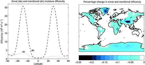
The atmospheric model consists of vertically integrated energy and moisture balance equations and is forced by seasonally varying solar insolation and reanalysis winds from the National Centers for Environmental Prediction (NCEP; Kalnay et al., 1996). Atmospheric moisture transport is achieved through diffusion and advection by winds. More specifically, the moisture advection scheme applies a wind field calculated as the weighted average of the NCEP long-term monthly mean winds (from atmospheric levels below 10,000 m) (Kalnay et al., 1996). The weighting of the NCEP winds decreases exponentially with height to account for the exponential decrease in atmospheric water vapour with height. Superimposed wind anomalies are calculated dynamically as a function of surface temperature gradients, as described by Weaver et al. (2001). Moisture diffusion coefficients vary with latitude and are held constant in time. Zonal diffusivity is essentially symmetric around the equator and achieves peak values between 40° and 50° in both hemispheres. In contrast, meridional diffusivity is higher in the southern hemisphere, with peak values occurring between 40° and 50°S. Meridional (zonal) diffusivity ranges from 0.8 to 3.56 × 10⁶ m² s⁻¹ (0.05 to 3.1 × 10⁷ m² s⁻¹). The parametrization of atmospheric moisture diffusivity is different from the atmospheric moisture diffusion coefficient using diffusive + advective moisture transport, K (ADVDIF), originally described in Weaver et al. (2001). After the implementation of the dynamic vegetation scheme by Meissner et al. (2003), the diffusivity scheme was modified to its current form. Here, diffusivity varies only with latitude and K consists of different coefficients for meridional and zonal moisture diffusivity (see left panel in Fig. 1).

Fig. 1 Model atmospheric water vapour diffusivity. Variation of initial model zonal (de) and meridional (dn) diffusivity with latitude (left panel) and percentage change in zonal and meridional diffusivity for relative to (maximum reduction is 0.25%) (right panel).

The land-surface model employs a dynamic vegetation land surface scheme (Met Office Surface Exchanges Scheme (MOSES)/Top-down Representation of Interactive Foliage and Flora Including Dynamics) using a one-layer soil moisture (leaky bucket) representation (Meissner et al., 2003), which runs off to one of thirty-two rivers according to the river catchment basin where the grid cell is located. Snow may accumulate as a single, height-varying layer in the land surface model, with snowmelt either replenishing soil moisture or contributing to river runoff when the soil is saturated.

The standard thermodynamic–dynamic sea-ice model (Semtner, 1976; Hibler, 1979) employed here consists of sub-gridscale ice-covered and open-ocean categories, with a height-varying sea-ice layer and elastic viscous plastic ice rheology (Hunke and Dukowicz, 1997). Snow falling on sea ice may accumulate as a single height-varying snow layer.

b Implementation of Oxygen Isotopes

Moisture is modelled explicitly as humidity in the atmospheric model, soil moisture and lying snow in the land-surface model and ice and overlying snow in the sea-ice model. The existing model moisture was assumed to consist of and equivalent reservoirs were added. On land, is represented in soil moisture and in snow lying on the land surface. In the sea-ice model, is represented in the ice layer and the overlying snow layer.

The rigid-lid ocean model employs a constant-volume assumption such that salt fluxes are substituted for moisture fluxes, necessitating the addition of both and as ocean tracers (as in Tindall et al. (2009)). At the sea surface, variations in isotopic content result from evaporation, precipitation, sea-ice growth and melt and inputs of river runoff. Away from the sea surface, and are essentially passive tracers resulting from the absence of subsurface sources or sinks. While water–rock interactions occurring at the seafloor fractionate oxygen isotopes in seawater, with low (high) temperature interactions producing depleted (enriched) seawater (Walker and Lohmann, 1989), these water–rock isotope exchange processes are considered to be in isotopic balance on the time scales applicable to our model simulations (i.e., less than 10⁵ years, contrasted with a shift of 1‰ every 10⁸ years described by Walker and Lohmann (1989)).

Following the implementation of stable water isotopes in other models (e.g., Hoffmann et al., 1998; Lee et al., 2007; Tindall et al., 2009), undergoes exchange across surface boundaries and fractionation during the appropriate phase changes, summarized in Table 1.

Table 1. Oxygen isotope fractionation during surface exchanges and phase changes. R = mass ratio H₂ ¹⁸O/H₂ ¹⁶O for precipitation (p), atmospheric vapour (v), ice (i), evaporation (e), seawater (oc) and soil moisture (s); α = fractionation factor, with α_eq and α_kin the equilibrium and kinetic fractionation factors (respectively); S = supersaturation parameter; T = temperature (in K for α_eq expressions, °C for S expression); D, D_i = H₂ ¹⁶O , H₂ ¹⁸O diffusivities; h = relative humidity; ρ _i /ρ = ratio of effective resistances for H₂ ¹⁸O and H₂ ¹⁶O (in the Craig and Gordon (1965) linear-resistance type model for evaporation of isotopic species); following Gat (1996), evaporation under open-water conditions is represented in the selection of constants θ = 0.5 and n = 0.5, while C_D = 28.5‰.

Process	Fractionation
Condensation, vapour-liquid (T ≥ −10°C)		(Majoube, 1971a)
Condensation, vapour-ice (T < −10°C)		(Majoube, 1971b)
Condensation, vapour-ice (T < −20°C)		(Majoube, 1971b)
		(Jouzel and Merlivat, 1984)
		(Jouzel et al., 1987)
Evaporation from sea surface		(Majoube, 1971a)
		(Gat, 1996)
Evaporation from soils
Freezing (sea-ice growth), liquid-ice		(O'Neil, 1968)
Sublimation, solid-vapour
Transpiration, liquid-vapour	R e = R s

1 Condensation

Precipitation forms in the model when atmospheric relative humidity is above 85%. Precipitation occurs under Rayleigh (or open system) conditions, because rain or snow that forms in the model is immediately removed from the atmosphere without any exchange with ambient vapour (see Dansgaard (1964) and Joussaume and Jouzel (1993) for treatment of modelling precipitation in open versus closed systems). At temperatures above −20°C, all precipitation forms in thermal equilibrium with the atmospheric vapour and is enriched relative to the vapour by α, the equilibrium fractionation factor, such that . As in Jouzel et al. (1987), we assume the isotopic vapour condenses to liquid at or above −10°C and forms a solid otherwise. We apply the appropriate equilibrium fractionation factors from Majoube (1971a, 1971b) for vapour–liquid and vapour–solid transitions, respectively. An additional kinetic fractionation is included at temperatures below −20°C to account for the effects of differential molecular diffusion of and through a supersaturated layer surrounding an ice crystal (described in Jouzel and Merlivat (1984)). After Schmidt et al. (2005), the supersaturation is parameterized as (T is air temperature in °C) (such that S _ice varies between 1 and the ratio of saturation vapour pressures of ice to water (see Jouzel et al. (1987)). Fractionation effects during condensation are summarized in Table 1.

2 Evaporation

Fractionation during evaporation from the sea surface depends on the moisture and isotope gradients at the ocean–atmosphere interface and takes into account both equilibrium effects (i.e., temperature-dependent) and kinetic effects (i.e.,resulting from the differences in molecular diffusivity for and ). The isotopic fluxes in evaporation are well described by the Craig-Gordon evaporation model (Craig and Gordon, 1965), which is based on a Langmuir resistance model. In the Craig-Gordon model, the evaporative flux of (E) is a simple function of the humidity gradient between the sea surface boundary (where relative humidity is equal to one) and aloft (characterized by relative humidity h). The evaporative flux driven by the humidity gradient is reduced by a resistivity parameter, ρ, such that . Likewise, the evaporative flux of (E_i ) includes the additional assumption that the vapour at the sea surface boundary is in isotopic equilibrium with the seawater (therefore equal to ), while the atmospheric water vapour aloft has an isotopic content of R_v , giving . As discussed in Gat (1996), the kinetic fractionation effects resulting from the differential molecular diffusion in air for and are included in the resistivity coefficients. The resulting ratio of and in evaporation, or R_e , is simply equal to E_i/E, shown in Table 1.

When snow or ice sublimates, the entire sublimated layer is removed to the atmosphere and no fractionation occurs. Likewise, transpiration by plants communicates unfractionated root water (i.e., soil moisture) to the atmosphere (Gat, 1996). Evaporation from bare soil is also returned to the atmosphere without fractionation. While evaporation from a soil column should include fractionation in theory, this process is neglected for the sake of simplicity (following most models). Because bare soil evaporation is small compared to the total evaporative flux; this simplification should have a minor effect. Fractionation processes during evaporation are summarized in Table 1.

3 Moisture transport over elevation

In an earlier version of the model, precipitation was not sufficiently depleted when atmospheric humidity was transported over grid cells containing higher land elevation (relative to the low elevation precipitation, compared to both observations and AGCMs with multiple levels in the vertical). The likeliest explanation is that because the UVic model does not resolve atmospheric vertical convection, moisture transported to higher elevations would simply condense at colder temperatures from overly enriched vapour (as opposed to the depleted vapour aloft found in AGCMs, presumably via distillation from vertical air motion). To address this problem, we decreased the diffusion of by an elevation-dependent amount. The difference in atmospheric diffusivity between and is zero over ocean points, negligible over low elevation (most continental points) and important only over significant high elevation regions (Antarctica, Greenland and the Himalayas), shown in Fig. 1 (right panel). While the highest model elevation is found in eastern Antarctica (which is more than 1000 m higher than central Greenland), the percentage reduction is larger in Greenland because the initial absolute value of the meridional moisture diffusivity coefficient is smaller at 70°N than at 82°S.

3 Pre-industrial Equilibrium Simulation

The model pre-industrial climatology discussed here results from a 5 kyr simulation with constant boundary conditions of year 1800 orbital configuration and solar forcing and a pCO₂ of 283.87 ppm. The ocean model was initialized to 0.1‰, the atmospheric humidity to −10‰ and other water reservoirs to 0‰.

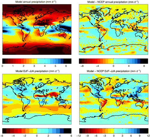
The UVic ESCM present-day climatology was fully described by Weaver et al. (2001). For reference, the model (pre-industrial) surface air temperature and precipitation (both annual mean and seasonal variation, defined as DJF−JJA) are presented in Figs 2 and 3. The differences between the model fields and the NCEP 40-year reanalysis (1957–96) (Kalnay et al., 1996) fields are included to highlight model-data discrepancies, which could shift the resulting distribution of isotopes.

Fig. 2 Model surface air temperature climatology. Temperature (°C) in the annual mean UVic model pre-industrial simulation (top left panel), the difference between the model and NCEP reanalysis annual means (top right panel), seasonal variation in the UVic model (DJF−JJA) (bottom left panel), and the difference in seasonality between the model and NCEP reanalysis DJF−JJA.

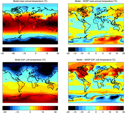
Fig. 3 Model precipitation climatology: precipitation (mm d⁻¹) in the annual mean UVic model pre-industrial simulation (top left panel), the difference between the model and NCEP reanalysis annual means (top right panel), seasonal variation in the UVic model (DJF−JJA) (bottom left panel) and the difference in seasonality between the model and NCEP reanalysis DJF−JJA.

The model and NCEP annual average temperatures are very similar (Fig. 2). The simulated global annual mean temperature (area-weighted) is 13.28°C and the equivalent NCEP value is 13.81°C (using NCEP data interpolated to the UVic model grid spacing). Eastern Antarctica, northeastern North America and northeastern Asia are warmer in the model relative to observations, with the largest discrepancy seen in eastern Antarctica, where the simulated annual mean value temperature is 16.66°C warmer than the NCEP value. The largest negative discrepancy is located in western Antarctica, where the modelled annual mean temperature is 13.42°C cooler than the NCEP value. The seasonal difference in temperature (DJF−JJA) is reduced in the model relative to NCEP (Fig. 2, bottom right panel). The largest model-NCEP seasonality anomalies are located over land (especially over northern hemisphere continents and eastern Antarctica, with maximum anomalies of –19.36°C and +18.25°C in eastern Antarctica and northeastern Asia, respectively), while most of the global ocean exhibits only small differences in seasonality. The model-NCEP seasonality difference may be enhanced over land due to the neglect of vertical atmospheric processes in the model, which is likely to propagate greater error over land (because topography may induce complex atmospheric responses) and due to propagation of model errors in continental soil moisture and moisture fluxes.

With respect to precipitation, the model reproduces the global pattern of observed annual precipitation and the model global mean precipitation rate is close to the observed value (2.89 and 2.74 mm d⁻¹ respectively). The highest observed precipitation rates in the annual mean are underestimated by the model, such as in Amazonia (Fig. 3), a feature common across models. Differences in model and NCEP precipitation seasonality (DJF−JJA) between the model and the NCEP data are most pronounced over southern and eastern Asia, eastern North America, Central America and central Africa.

In the following sections we focus on the modelled distribution of oxygen isotopes in moisture fluxes and seawater and compare the modelled isotope patterns to observations.

a Isotopes in Precipitation

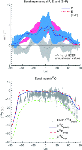
Dansgaard (1964) described a set of isotope effects relating the oxygen isotopic content in precipitation (δ¹⁸O_precip) to factors including precipitation amount, latitude, surface air temperature, distance from the coast and altitude. These observed relationships are all produced by the total amount of moisture lost from an air mass (known as rain-out) as it travels away from its moisture source (Rozanski et al., 1993). The degree to which the UVic model can capture these observed patterns in δ¹⁸O_precip is a function of the accuracy of the modelled temperature, evaporation and precipitation fields, as well as the representation of moisture transport. As shown in Fig. 4 (top panel), model annual zonal mean moisture flux quantities (here, precipitation, evaporation and E−P, the difference between evaporation and precipitation) all fall within one standard deviation of NCEP annual mean values at all latitudes.

Fig. 4 Zonal mean fluxes of moisture and isotopes. Zonal annual mean precipitation (solid blue line), evaporation (red dashed-dotted line) and E-P (dark grey dashed line) in the UVic model, superimposed on the range of the NCEP zonal annual mean values ±1σ observed in precipitation (blue bars), evaporation as calculated from NCEP latent heat fluxes (pink bars) and E-P (light grey bars) (top panel) and zonal annual mean δ¹⁸O in precipitation (solid blue line), evaporation (red dashed-dotted line) and atmospheric water vapour (green dashed line) (bottom panel) in the model, superimposed on all available annual mean precipitation δ¹⁸O observations in GNIP data (grey diamonds), separated into 1/4 degree latitude bins. NCEP reanalysis data are from Kalnay et al. (1996); GNIP δ¹⁸O data are provided by IAEA (2006). Figure based on Fig. 12 in Lee et al. (2007) and Fig. 1 in Zhou et al. (2008).

Observations of isotopes in precipitation have been collected at several hundred stations since the 1960s, forming the Global Network of Isotopes in Precipitation (GNIP) (IAEA, 2006). To compare the model against GNIP observations, all GNIP stations for which the weighted annual average of δ¹⁸O and surface air temperature are available for individual years (between 1961 and 2001) are selected (369 stations). The UVic model grid cell located nearest each GNIP station was determined, and the annual mean isotope content and surface air temperature from that grid location are sampled from the model.

While the model zonal mean isotopic content in precipitation falls within the range of the GNIP long-term mean δ¹⁸O values at most latitudes (with the exception of the latitude band –30°S to –70°S) (Fig. 4, bottom panel), the zonal mean δ¹⁸O_precip is more enriched than GNIP observations, on average. This model enrichment may be explained by overly enriched vapour δ¹⁸O (δ¹⁸O_vap) where condensation forms in the atmospheric model. The model zonal mean δ¹⁸O_vap is quite similar to the National Center for Atmospheric Research Community Atmosphere Model (NCAR CAM2) AGCM surface (lowest) layer of δ¹⁸O_vap (see Lee et al. (2007), their Fig. 12b), but where the model forms condensation from the bulk atmospheric δ¹⁸O_vap, in an AGCM condensation may form aloft (in one of more than 20 vertical atmospheric layers), and δ¹⁸O_vap decreases with height. The latitude band –30°S to –70°S corresponds to the latitude of least land surface. The large ocean area may increase the relative component of local oceanic evaporation contributing to δ¹⁸O_vap and can decrease the effect of reduced diffusivity (which is a function of elevation, see Fig. 1) in this region. The model δ¹⁸O_precip globally averaged value of −7.5‰ is within the range of values reported from AGCMs (−6 to −7.5‰, see Table 2).

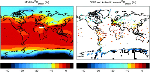
Figure 5 maps both the modelled mean annual δ¹⁸O_precip and the long-term mean values at each GNIP station supplemented with Antarctic surface snow isotopic observations from Masson-Delmotte et al. (2008), interpolated to a UVic model grid to enable comparison. Consistent with the latitude effect, δ¹⁸O_precip decreases poleward in the model, reaching a minimum value of −47.1‰ in central Antarctica (in the northern hemisphere, a minimum of −26.2‰ is achieved in northern Greenland). A local enrichment (+4.4‰) occurs in southeast Asia on the lee side of the Himalayas. This feature is not found in the observations and likely results from the elevation-dependent modification of diffusivity. While the model δ¹⁸O_precip exhibits close to observed latitudinal patterns, regional discrepancies between modelled and observed patterns are evident. For example, the regions of northern North America, northern Europe and southern South America are too enriched in the model. Otherwise, the model is generally consistent with observations throughout Asia (not including the aforementioned enrichment east of the Himalayas), Australia, Africa and Antarctica. The root mean square error (RMSE) provides a quantitative measure of the differences between the modelled annual average δ¹⁸O_precip and the GNIP long-term mean values (interpolated to the UVic model grid), which for individual stations ranges from a minimum of 0.0‰ to a maximum of 18.2‰, with an expected value of 4.1‰.

Fig. 5 δ¹⁸O in precipitation. Annual average δ¹⁸O in present-day precipitation for the UVic model (left panel) and observations from GNIP (IAEA, 2006) (long-term time averages shown) and Antarctic surface snow (Masson-Delmotte et al., 2008) datasets, interpolated to a UVic model grid (right panel). Observational values are plotted at a slightly larger size than the actual grid cell (130%) for improved visualization.

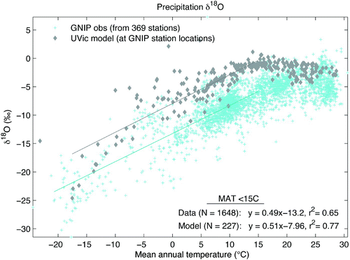
For mean annual temperatures below 15°C (excluding extreme outliers below –21°C), the spatial relationship between temperature and δ¹⁸O_precip is very similar in slope between model (sampled at GNIP station locations) and GNIP data, shown in Fig. 6. The model slope of 0.51 is very close to the slope of 0.49 for the data, with r ² values of 0.77 and 0.65, respectively. Plotted values include all years of GNIP station data with annual average surface temperature and weighted δ¹⁸O_precip (N =3085) and mean annual surface air temperature and δ¹⁸O_precip from the UVic model at GNIP station locations (N =369).

Fig. 6 Temperature – δ¹⁸O spatial relationship. Mean annual temperature and δ¹⁸O in precipitation are plotted for observations at GNIP stations for each available year (blue crosses, N =3085) and the UVic model at GNIP station locations (grey diamonds, N =369). The linear fit and trend line for GNIP and model values with mean annual temperature less than 15°C (excluding outliers below –21°C) are indicated (blue line, N =1648 and grey line, N =227, respectively).

1 Discussion of model ¹⁸ O _precip

In order to explain model-data discrepancies in δ¹⁸O of precipitation (and, by extension, seawater), here we consider the impacts of several parameterizations in the atmospheric model on condensation and moisture transport as they relate to isotopes. These parameterizations are necessary to achieve the desired model computational efficiency and speed but require the simplification of several atmospheric processes. First, condensation forms in the model when relative humidity exceeds 85%. This precipitation is instantaneously removed from the atmospheric column and is subsequently added to the surface moisture flux. In effect, partial re-evaporation of falling precipitation is neglected. Without partial re-evaporation (which adds depleted water vapour), local precipitation is more depleted, while the remaining vapour is more enriched. The overall result of more enriched remaining vapour would tend to dampen the “latitude effect” in the model.

Second, condensation occurs in the model at surface air temperatures (adjusted for elevation over land by a lapse rate). Since condensation forms at warmer surface temperatures as opposed to cooler temperatures aloft, this yields a smaller effective fractionation. Smaller fractionation during condensation produces slightly more depleted local precipitation and more enriched remaining atmospheric water vapour (as in the case of neglecting re-evaporation).

Third, model precipitation derives from a vertically integrated atmospheric column, such that the atmospheric moisture is essentially well-mixed with respect to isotopes. This assumption precludes a description of vertical motion of air masses (and their associated condensation) or vertical differentiation of isotopes. In contrast, condensation forms in the earth's atmosphere at variable heights and the atmospheric column is characterized by variable δ¹⁸O and temperature (typically, with more isotopically depleted and colder values aloft) (for example, see discussion in Lee et al. (2007) and their Fig. 15). The result is that the water vapour from which condensation forms (the well-mixed atmospheric column) is likely to be more enriched in the model (than vapour at an altitude of several thousand metres, for example), and in turn, precipitation would be more enriched. However, isotopes in precipitation are generally observed to be in equilibrium with the water vapour in the lowest layer of the atmosphere, which may partially account for the model's capturing of the observed large-scale patterns in δ¹⁸O_precip.

The above processes may create opposing isotopic effects, with local precipitation becoming more enriched because of a more enriched bulk water vapour, and/or less enriched based on both the smaller fractionation factor resulting from a warmer surface temperature and the neglect of re-evaporation. The net effect of neglecting these processes may be to reduce variability in model δ¹⁸O_precip in regions where vertical moisture transport, re-evaporation of falling droplets and high-altitude condensation are important. As seawater surface δ¹⁸O variability mainly depends on the variability of δ¹⁸O in moisture fluxes at the sea surface (and river inputs are essentially a signal of average δ¹⁸O_precip over the drainage basin), δ¹⁸O_sw may be reduced in variability by these processes as well (discussed below).

b Isotopes in Seawater

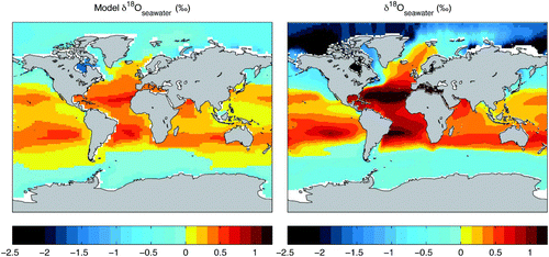
The distribution of oxygen isotopes at the ocean model surface reflects the isotopic fluxes occurring during evaporation from the sea surface, precipitation, additions of river runoff and sea ice melt and brine production, in addition to the effects of transport and mixing of water masses. The model δ¹⁸O at the sea surface (top 50 m) is compared with the interpolated observations (averaged over the top 50 m) (LeGrande and Schmidt, 2006) based on the Goddard Institude for Space Studies (GISS) Global Seawater Oxygen-18 Database (Schmidt et al., 1999) in Fig. 7. Because maximum variability is located nearest the sea surface and the upper layer of the UVic ocean model is 50 m deep, the model–data comparison of the top 50 m is appropriate in assessing model variability. The oxygen isotope composition of seawater (δ¹⁸O_sw) in the model displays the same broad features found in the observations. Surface water is more depleted at high latitudes than in low latitudes. Net evaporative regions (where ) contain more positive δ¹⁸O_sw values. The Atlantic, for example, contains more enriched δ¹⁸O_sw values than the Pacific. These observed large-scale patterns suggest that the model produces a reasonable first-order distribution of moisture fluxes. A model–data discrepancy, however, is apparent in the absolute range of surface δ¹⁸O_sw values, narrower in the model than in observations. This reduced variability in surface δ¹⁸O_sw may result from the treatment of moisture transport and condensation in the atmospheric model, which affect seawater via precipitation and river runoff.

Fig. 7 Sea surface δ¹⁸O. Surface seawater δ¹⁸O in the UVic model (annual mean of surface ocean model level (depth 50 m)) (left panel) and the gridded δ¹⁸O seawater dataset (LeGrande and Schmidt, 2006) (averaged over the top 50 m) (right panel).

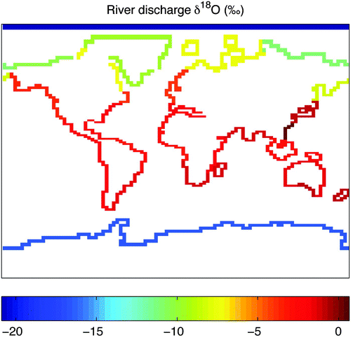
Because precipitation and snowmelt are returned immediately to the ocean (once soil moisture is saturated) via river runoff, it is useful to compare observations of river runoff δ¹⁸O (δ¹⁸O _r ) with model values. Yi et al. (2012) report annual discharge and weighted mean δ¹⁸O _r data collected between 2003 and 2006 from six major Arctic rivers as part of the Pan-Arctic River Transport of Nutrients, Organic Matter and Suspended Sediments (PARTNERS) project. The most depleted runoff originates in the Kolyma River (−22.18‰), the most enriched in the Ob River (−14.85‰), and the annual weighted mean δ¹⁸O_r value for all six rivers (Mackenzie, Kolyma, Lena, Yenlsey, Ob and Yukon) is −18.72‰. In the model, river discharge into the Arctic Ocean ranges from −7.2‰ to −11.0‰ and only runoff from the (non-physical) island at the pole is as depleted as observations (−20.9‰). The mean annual Antarctic river discharge in the model is −16.8‰ (Fig. 8).

Fig. 8 Annual mean δ¹⁸O in model river discharge (‰). River runoff from 32 river basins is discharged at coastal points (described in Weaver et al. (2001)).

1 Salinity- ¹⁸ O _sw relationships

Both seawater δ¹⁸O and salinity are shifted in the same direction by processes occurring at the ocean surface (with the noted exception of sea-ice growth and melt (e.g., Strain and Tan, 1993)), resulting in a linear relationship between the two quantities. For example, evaporation (precipitation) typically increases (decreases) both salinity and δ¹⁸O_sw. We compare the slope of the best fit line for the salinity-δ¹⁸O_sw data sampled from the model to that sampled from the same region in the observations.

To best describe water mass characteristics, it is standard practice to assess the properties of upper water (< 400 m), intermediate water (400–2500 m) and deep water (> 2500 m) separately. To characterize the upper water column, we define surface waters as the top 400 m and in the model the top four ocean levels, which corresponds to a depth of 380 m, within the salinity range 28 to 38. Observations from the same coordinate and depth level are time-averaged. The model salinity and δ¹⁸O_sw are sampled from every ocean grid cell, resulting in a larger sample size from the model relative to the observations.

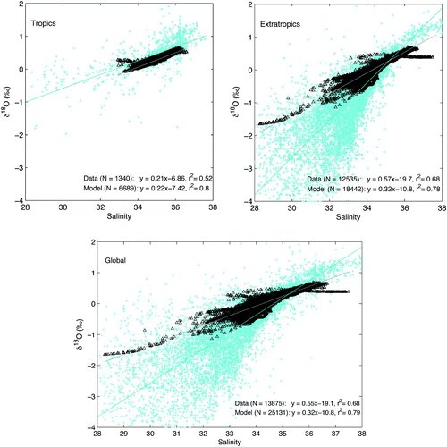
Tropical surface waters (between 20°N and 20°S) have very similar relationships between model and observed salinity-δ¹⁸O_sw relationships (Fig. 9). In the tropical Atlantic, we find a model slope (in salinity-δ¹⁸O space) of 0.19 (r ²=0.74) and an observed slope of 0.18 (r ²=0.50). In the tropical Pacific, we find salinity-δ¹⁸O slopes of 0.23 (r ²=0.96) in the model and 0.24 (r ²=0.77) in the observations. The similarity between the model and observed slopes decreases slightly in the tropical Indian Ocean surface waters which have a salinity-δ¹⁸O slope of 0.16 (r ²=0.55) in the model and 0.24 (r ²=0.57) in the data. In comparison, the extratropical surface water salinity-δ¹⁸O relationship is weaker in the model than in the observations. The model slope of 0.32 (r ²=0.78) is significantly less than the observed slope of 0.57 (r ²=0.68). Similarly, the surface waters of the global ocean have a slope of 0.32 (r ²=0.79) in the model, which is less than the slope of 0.55 (r ²=0.68) observed in the data (Fig. 9).

Fig. 9 Salinity-δ¹⁸O spatial relationships in seawater. Surface water salinity-δ¹⁸O relationships found in the modelled pre-industrial annual mean (black diamonds) and the Global Seawater Oxygen-18 Database (Schmidt et al., 1999) (blue crosses) in the tropics (20°S–20°N) (top left panel), extratropics (> 20°N and S) (top right panel), and in the global surface waters (bottom panel). The linear fit to the observations (blue line) and model values (grey line) are indicated in the lower right.

Intermediate waters (400 to 2500 m) have a global mean salinity and δ¹⁸O_sw of 34.7 and 0.10‰ in the model, indistinguishable from the GISS Seawater Oxygen-18 Database values of 34.9 and 0.10‰ for intermediate water (N > 5400). The salinity-δ¹⁸O_sw spatial relationship in global intermediate waters is slightly reduced in the model compared to the data (slopes of 0.23 (r ²=0.52) and 0.39 (r ²=0.76), respectively). In the model, as in the observations, deep water (> 2500 m) is more saline and more enriched in in the North Atlantic than in the other ocean basins. While observations reveal the global deep ocean to be, on average, 0.3 to 0.45‰ more negative than deep water in the North Atlantic, the difference in the model is less dramatic, approximately 0.1‰.

4 Last Glacial Maximum equilibrium simulation

a Set-up and Initialization

A 5 kyr simulation was performed using constant boundary conditions for the Last Glacial Maximum (LGM), including an orbital configuration corresponding to 21 kyr BP, atmospheric pCO₂ of 189.65 ppm and increased elevations where ice had accumulated on land (following the Peltier (1994) ICE-4G reconstruction). The LGM simulation employs the same NCEP wind forcing used for the pre-industrial simulation, although the superimposed dynamic wind feedback component (a function of surface temperature gradients) is different. Atmospheric moisture diffusivity is unchanged from the pre-industrial simulation. Additionally, LGM surface albedo is increased in gridcell locations corresponding to the expanded prescribed ice sheet cover and the increased snow cover (both with an albedo of 0.80). The model was initialized using a previous LGM simulation such that the ocean and climate physical parameters were already at quasi-equilibrium values.

In order to initialize the water isotope reservoirs, recent estimates of the difference between LGM and present-day values were considered. By applying a pore water diffusion model to a deep western Pacific sediment core, Schrag et al. (1996) estimated a 1.0 ± 0.25‰ LGM seawater enrichment, relative to present day. Duplessy et al. (2002) considered the full range of LGM sea level estimates (120–140 m) and using the same methods (i.e., Schrag et al., 1996; Adkins and Schrag, 2001) concluded that the LGM ocean was enriched relative to present day by 0.95–1.08‰. Duplessy et al. (2002) further assessed all other robust methods for estimating the LGM seawater isotopic shift and determined a best estimate of 1.05±0.20‰. We therefore initialized the LGM ocean to 1.1‰ above the pre-industrial seawater initial value of 0.1‰. Ice on land was set to −30‰, atmospheric water vapour to −10‰ and other water reservoirs (sea ice, snow lying on land and sea ice and soil moisture) to 0‰.

b LGM Climatology

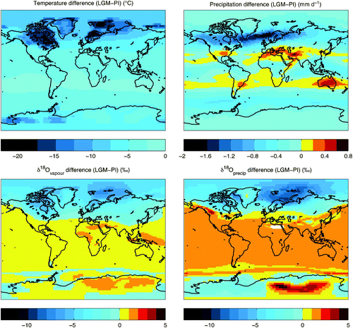
The modelled LGM climatological patterns (e.g., surface air temperatures and ocean temperatures) are very similar to the LGM simulation described by Weaver et al. (2001). As shown in Fig. 10, the LGM global mean temperature is 4.08°C cooler, and the global mean precipitation is 0.19 mm d⁻¹ lower relative to the pre-industrial (PI). Precipitation is slightly enhanced only in a narrow mid-latitude band in each hemisphere. Climatological mean values for the LGM and Pre-industrial (PI) simulations as well as the LGM-PI differences are presented in Table 3.

Fig. 10 Model LGM-PI climatological and isotopic differences. Annual mean difference between LGM and PI surface air temperatures (top left panel), precipitation (top right panel), δ¹⁸O in atmospheric water vapour (bottom left panel), and δ¹⁸O in precipitation (bottom right panel).

As in previous LGM simulations with the UVic model, the maximum meridional overturning streamfunction is lower in the pre-industrial simulation (14.4 Sv in the LGM compared to 21.75 in the pre-industrial), sea-ice cover is greater (2.5 × 10¹³ m² during the LGM simulation compared to an annual mean of 2.2 × 10¹³ m² in the pre-industrial simulation) and the sea surface temperature (SST) is lower (the largest decrease, > 8°C, is found in the northeast Atlantic Ocean, while the mean tropical SST change is −2.4°C) except in the polar oceans where expanded sea-ice cover decreases heat loss to the atmosphere (not shown, see Figs 37–39 in Weaver et al. (2001)).

c Isotopes in LGM Precipitation

Changes in the distribution of isotopes in precipitation in the LGM simulation relative to the pre-industrial simulation ( ) may result from changes in the rate, timing (e.g., seasonality), and/or isotopic content of surface moisture fluxes, the relative enrichment of the primary moisture source (the surface ocean) and changes in moisture transport. Temperature change has a direct effect on δ¹⁸O_precip in modifying the equilibrium fractionation factor during condensation (with cooler temperatures producing larger fractionation) but otherwise has an indirect influence on δ¹⁸O_precip through its impact on moisture fluxes and transport. The LGM climate exhibits cooler surface temperatures (notably in the northern hemisphere), increased subtropical precipitation coupled with decreased precipitation elsewhere (shown in Fig. 10) and an enriched surface ocean (as a result of the expanded continental ice). This set of conditions is likely to produce enriched atmospheric vapour and precipitation at low latitudes (a consequence of the enriched source evaporate) and increased rain-out of isotopes in mid- and high latitudes, or an increased latitude effect (a function of both cooling and the precipitation changes).

Atmospheric water vapour and precipitation are slightly more enriched at low latitudes in the LGM simulation compared to the pre-industrial simulation (Fig. 10). A similar slight increase in low latitude δ¹⁸O_precip is found in other models (e.g., the isotope-enabled LMD (LMDZ-iso) AGCM results shown in Figs 12–13 in (e.g., Risi et al., 2010). The model is able to capture the LGM depletion in northern hemisphere high latitudes, but the magnitude of the depletion is smaller over northern North America than in the LMDZ-iso AGCM. For example, the model maximum decrease in annual mean δ¹⁸O_precip is 10.6‰, while in the LMDZ-iso the LGM precipitation falling in the Hudson Bay region is depleted by more than 15 to 25‰ relative to present day (depending on which LGM SST forcing is applied).

Fig. 11 Model and reconstructed LGM-PI δ¹⁸O_precip differences. Annual mean difference between LGM and PI δ¹⁸O in precipitation in the model (top left panel) and the reconstructions, interpolated to a UVic model grid (top right panel), with a scatterplot of reconstructed versus model values (sampled from the model at the locations of the reconstructed values) (bottom panel). A 1:1 line is included. Reconstructed values are plotted at a slightly larger size than the actual grid cell (130%) for improved visualization. LGM–PI data are summarized in Table 3. Complete references are provided in Table 2 in Duplessy et al. (2002) and Table 2 in Risi et al. (2010).

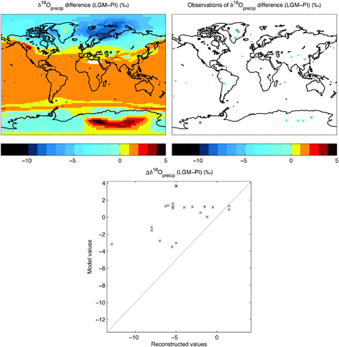
Fig. 12 Contributions to LGM–PI annual difference in model precipitation isotopic content (‰). Component of LGM–PI shift in δ¹⁸O_precip resulting from the temperature-dependent equilibrium fractionation factor in condensation (top left panel), resulting from the enrichment of the glacial ocean (by 1.1‰) (top right panel), and resulting from other processes (bottom panel), which is the combined effect removed from the LGM–PI shift.

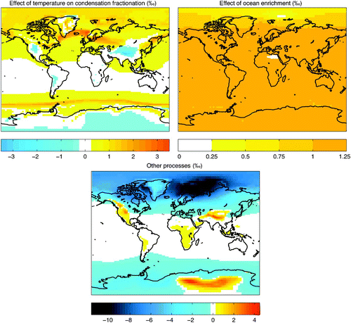
Fig. 13 LGM–PI differences in seawater δ¹⁸O (‰) in the ocean model. Total annual mean difference between modelled LGM and pre-industrial δ¹⁸O_sw (includes ocean enrichment caused by increased continental ice volume) (left panel) and with the component due to ocean enrichment removed (right panel) for surface waters (weighted average value from 0 to 380 m) (top panels), and for a mid-intermediate water layer (980 to 1240 m) (bottom panels).

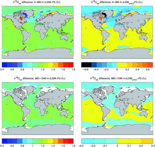
Table 2. Global general circulation and intermediate complexity models with stable water isotopes. If it was reported, the global mean δ¹⁸O_precip value is given (NA if isotopes are not explicitly modelled in atmospheric precipitation).

Models	Reference	Global mean δ^18Oprecip
Atmospheric GCMS
ECHAM3	Hoffmann et al. (1998)	(N. Atl. vapour −12‰)
ECHAM4	Werner et al. (2001)
ECHAM5	Werner et al. (2011)
GENESIS	Mathieu et al. (2002)
GISS	Jouzel et al. (1987)
ICM	Yoshimura et al. (2003)
LMD	Joussaume et al. (1984)
LMDZ4*	Risi et al. (2010)	−7.56‰
MUGCM	Noone and Simmonds (2002)
NCAR CAM2	Lee et al. (2007)
NCAR CAM3	Noone and Sturm (2010)
ECPC GSM	Yoshimura et al. (2008)**	−6.5 to −7.0‰
Ocean GCMs
CCM3	Delaygue et al. (2000)	NA
GISS	Schmidt (1998)	NA
AOGCMs
GENESIS-MOM	Zhou et al. (2008)	−7.1‰
GISS ModelE	Schmidt et al. (2007)	−6.0‰ (vapour −13.0‰)
HadCM3	Tindall et al. (2009)
EMICs
CLIMBER-2	Roche et al. (2004a)	NA
GENIE-1	Marsh et al. (2006)	NA
UVic ESCM	This work	−7.5‰
*LMDZ4 global δ^18O mean value is for AMIP simulation 1979 annual mean (Risi et al., 2010).
**Yoshimura et al. (2008) provide a range of monthly global mean δ^18Oprecip for ECPC GSM.

The model LGM-PI depletion in the southern hemisphere high latitudes is rather weak (less than 2.5‰), and while one of the LMDZ-iso AGCM simulations produces an enrichment near the Antarctic coast (see Fig. 13 in Risi et al. (2010)), our model also simulates an enrichment over inland eastern Antarctica, in contrast with the depleted LMDZ-iso values. Relative to the pre-industrial simulation, eastern Antarctica in the LGM simulation is characterized by only small changes in ice thickness (increases of 100 to 500 m), temperature (see Fig. 4, top left panel), and precipitation (see Fig. 4, top right panel). Eastern Antarctica contains the highest southern hemisphere elevations, generally above 3000 m. It is likely that the model does not produce sufficient successive condensation (rain-out) between the evaporation of (slightly enriched) moisture from the sea surface and the formation of local precipitation, such that the model vapour entering this region is overly enriched.

We can compare model LGM δ¹⁸O_precip to the δ¹⁸O values measured from ice cores and cave deposits formed during the LGM (Table 3). Risi et al. (2010) compiled estimates from the most recently available ice core, cave deposit and aquifer records spanning the LGM (their Table 2). The compilation includes the isotopic content in ice measured in fifteen ice cores from high-latitude (Greenland and Antarctica), mid-latitude (Tibet) and low-latitude (South America) ice cores and the isotopic content determined at seven mid- and low-latitude cave and aquifer sites. The estimate of LGM δ¹⁸O_precip at each site may be characterized by various types of uncertainty, including dating uncertainty as noted by Risi et al. (2010).

Table 3. Climatological and isotopic annual mean values from the pre-industrial (PI) and Last Glacial Maximum (LGM) model equilibrium simulations, the difference between LGM and PI data (LGM-PI) and available reference data for comparison. Low and mid-latitudes refer to 0°−30°N, S and 30°−60°N, respectively. Where the reference time period is not specified, the value refers to the pre-industrial time period. For LGM-PI data references, see Table 2 in Risi et al. (2010) and Table 2 in Duplessy et al. (2002).

	PI	LGM	LGM-PI	Reference
Global
Surface air temp. (°C)	13.26	9.18	−4.08
Surface ocean temp. (°C)	17.86	15.57	−2.29
Precipitation (mm d^−1)	2.89	2.70	−0.19	2.74
δ^18Oprecip (‰)	−7.5	−7.4	0.1
δ^18Oprecip, marine (‰)	−4.2	−3.9	−0.3
δ^18Oprecip (‰)
Greenland
GRIP ice core	−16.7	−19.5	−2.8	−7
Camp Century ice core	−19.7	−22.9	−3.2	−12.9
Dye 3 ice core	−4.0	−7.5	−3.5	−5.5
Renland ice core	−10.5	−13.6	−3.0	−5
NGRIP ice core	−19.5	−20.7	−1.2	−8
Mid-latitude
England	−3.8	−3.8	0.0	−1.2
Guliya ice core	−4.6	−3.6	+1.0	−5.4
Dunde ice core	−6.7	−6.2	+0.5	−2
Sanbao and Hulu caves	1.2	2.1	+0.9	+1.5
Low-latitude
Stampriet aquifer	−1.4	−0.1	+1.3	+1.5
Huascaran ice core	−3.2	−1.9	+1.3	−6.3
Sajama ice core	−3.0	−1.7	+1.2	−5.4
Illimani ice core	−1.1	0.3	+1.4	−6
Botuvera cave	−1.3	−0.1	+1.2	−1.5
Santana cave	−1.5	−0.3	+1.2	−1.5
Rio Grande do Norte cave	−1.7	−0.5	+1.2	−0.5
Salar de Uyuni	−2.4	−1.3	+1.2	−4
Antarctica
Vostok	−36.5	−32.9	+3.6	−3 to –5
Byrd	−21.4	−23.0	−1.6	−8
Dome C	−28.8	−27.2	+1.6	−5.4
Dome B	−35.6	−32.0	+3.7	−5
Taylor Dome	−36.3	−35.1	+1.2	−3

The model LGM-PI difference in mean annual δ¹⁸O_precip indicates that the levels in the simulated LGM may not be as depleted as in the pre-industrial simulation as the reconstructed values suggest (Fig. 11). The reconstructed values are interpolated to a UVic model grid to permit direct model–data comparison. By plotting the LGM-PI change in the model mean annual δ¹⁸O_precip (sampled at the locations of the reconstructed values) against the reconstructed values with a 1:1 line, it is clear that the model is not as depleted in the LGM simulation compared to the pre-industrial simulation. The model–data discrepancy is largest in northwestern Greenland and eastern Antarctica and small at sites in southern Africa, south-eastern Asia, southern Greenland, England and along the east coast of South America. The likeliest explanation for the discrepancy in eastern Antarctica is insufficient rain-out in the model before precipitation forms, because of the proximity of the ocean and extreme topography where vertical processes are important (as noted above), but there is no clear single explanation for the misfit in northwestern Greenland.

To understand the processes affecting the LGM-PI shift in δ¹⁸O_precip better, one would ideally isolate portions of the forcing (including changes in temperature, precipitation, evaporation, atmospheric moisture transport and the isotopic content of seawater). Because of the constraint of conserving heat and moisture in the coupled model, partitioning the effects resulting from LGM-PI changes in temperature and moisture fluxes directly is not an option, because these are not independent. However, it is possible to assess the role of change in fractionation during condensation as a function of the LGM-PI temperature change, as well as that of an enriched LGM ocean.

Fractionation during condensation is a function of temperature, as described in Table 1 (α). By imposing a global field of pre-industrial surface air temperatures (specifically, the annual cycle using 5-day averages) within the LGM climate at equilibrium, the fractionation factor using the forced pre-industrial temperature (α*) is determined, as well as the resulting isotopic content of precipitation, which is saved offline (δ¹⁸O_precip*). The difference between δ¹⁸O_precip and δ¹⁸O_precip* gives the effect of the local temperature change on fractionation during condensation, shown in Fig. 12 (top left panel). With the aim of identifying the component of the LGM-PI shift in δ¹⁸O_precip caused by ocean enrichment, a second LGM simulation is performed in which seawater is initialized to the pre-industrial value (0.1‰), and the model is integrated 5 kyr to equilibrium. The difference in δ¹⁸O_precip between the enriched and unenriched seawater LGM simulations is plotted in Fig. 12 (top right panel).

Adding the effects of changes caused by temperature-dependent fractionation in condensation and seawater enrichment produces a combined effect (not shown), which when removed from the observed LGM-PI δ¹⁸O_precip signal, reveals the role of changes resulting from all other processes (bottom panel of Fig. 12). A significant portion of the low-to mid-latitude signal is explained by the combined effect, while clearly model changes in other factors (i.e., temperature, precipitation, transport, etc.) dominate the high-latitude LGM-PI shift in δ¹⁸O_precip.

d Isotopes in LGM Seawater

Changes in the distribution of oxygen isotopes in LGM seawater relative to the pre-industrial ( ) may occur as a result of changes in the amount of (relatively depleted) ice stored on land, ocean-atmosphere moisture exchanges, river inputs, sea-ice production and ocean circulation. As for changes in δ¹⁸O_precip (described above), changes in surface temperatures may result in both direct and indirect effects on δ¹⁸O_sw. Temperature changes cause changes in the (temperature-dependent) fractionation during evaporation from the sea surface (a direct effect) and also may cause a shift in the amount, timing, and/or geographical pattern of moisture fluxes at the sea surface (an indirect effect). The total LGM-PI shift in δ¹⁸O_sw is plotted in Fig. 13 for surface waters (depth-weighted average from 0 to 380 m, corresponding to the uppermost four ocean model levels) and a layer of intermediate water located at 980 to 1240 m depth in the model.

A second LGM simulation in which seawater is initialized to the pre-industrial value (0.1‰) is integrated 5 kyr to equilibrium, to represent an LGM state with an unenriched ocean (LGM_unenr). While the difference between the LGM and pre-industrial δ¹⁸O_sw represents the full expected change in δ¹⁸O_sw resulting from both climatic forcing and the buildup of continental ice (Fig. 13, left panel), the difference between the LGM_unenr and PI displays the same signal but without the influence of changes in continental ice volume (Fig. 13, right panels).

The LGM-PI difference in δ¹⁸O_sw ranges from 0.41 to 1.78‰ in surface waters and from 0.76 to 1.18‰ in the intermediate water layer (at 980 to 1240 m depth). When the enrichment effect caused by LGM continental ice accumulation is removed, the shift in δ¹⁸O_sw (LGM_unenr-PI) ranges from −0.69 to 0.68‰ in surface waters, and from −0.35 to 0.07‰ in the intermediate water layer. The modelled pattern of LGM_unenr-PI δ¹⁸O_sw is the product of changes in the physical state of the ocean, caused by water mass reorganization and changes in the magnitude, timing, and/or isotopic content of moisture fluxes at the sea surface.

5 Summary and conclusions

Stable water isotopes have been implemented in a range of atmospheric, oceanic and coupled models to date (see Table 2). Of these, few are fully coupled atmosphere–ocean models and fewer still are Earth system Models of Intermediate Complexity (or EMICs). The isotope-enabled UVic ESCM may fill a unique role in that it is an intermediate complexity model with a full ocean general circulation model (GCM) (as opposed to the EMIC CLimate-BiosphERe (CLIMBER-2) model with a zonally averaged three-basin ocean model), and the atmospheric and oceanic models are fully coupled for all fluxes (heat, moisture, oxygen isotopes, etc.).

When undertaking the implementation of and in the UVic model, we were initially skeptical as to whether the final distribution of δ¹⁸O would prove sufficiently realistic, given the simplified atmospheric subcomponent of the model and especially the model formulation of condensation (i.e., precipitation forms when relative humidity exceeds 85%).

Despite the similarity between the model and NCEP global annual mean temperature and precipitation, significant discrepancies are seen in the seasonal cycles of temperature and precipitation over broad continental regions. While the modelled annual and seasonal distribution of heat is fairly well represented over ocean regions, at low and mid-latitudes marine precipitation is both underestimated at its peak locations (e.g., the tropical western Pacific) and overestimated otherwise (e.g., the eastern Pacific to the west of the United States and Peru). For stable water isotopes, the lack of an explicit representation of atmospheric vertical structure and motions in the model may be the most significant model challenge. Isotopic fluxes resulting from dynamical, small-scale processes that are neglected in the model simply cannot be captured. Nevertheless, as noted below, our analysis indicates that the UVic model succeeds in capturing the broad pattern and magnitude of δ¹⁸O composition in mean annual precipitation and seawater.

We have performed long (5 kyr) equilibrium model simulations under pre-industrial and LGM boundary conditions and compared the resulting isotope fields with available data. In our evaluation of the model isotope distribution, we find that the model reproduces the large-scale patterns in precipitation. At the regional scale, the model is reasonably consistent with pre-industrial δ¹⁸O_precip observations throughout Australia, Africa, South America and across Asia (with the exception of the locally enriched area east of the Himalayas). The Antarctic region contains the maximum depletion in δ¹⁸O_precip both in the model and in observations, although precipitation in the model is not as depleted as observations from the Antarctic Surface Snow Dataset (Masson-Delmotte et al., 2008) suggest. Likewise, northern North America (Canada) is too enriched in the model relative to observations.

Under pre-industrial forcing, the model reproduces the observed large-scale sea surface isotopic patterns, including enrichment in evaporative regions and depletion at high latitudes, but the model is not as depleted as the observations in northern high-latitude seawater. This shortcoming is reflected in the model salinity-δ¹⁸O relationship in surface waters; while similar to the observations in the tropics, it is significantly weaker in extratropical surface waters. Model and observations are highly similar for global mean salinity and δ¹⁸O values in intermediate and deep waters.

Given these results, we suggest that the isotope-enabled UVic ESCM may be best utilized in performing simulations requiring integrations over long time scales, in combination with determining oxygen isotopic anomalies (between simulated climate states). The implementation of oxygen isotopes in the UVic ESCM adds new functionality to this intermediate-complexity model, allowing exploration of the potential processes determining the distribution of δ¹⁸O for a given climate. For example, one useful application may involve investigating variability in seawater isotopic content under distinct climate states. Finally, the model may be well suited to improving the interpretation of oxygen isotope records from ocean sediment cores.

Ocean sediment core δ¹⁸O records are generated from the seafloor accumulation of marine planktonic and benthic calcareous plankton (e.g., foraminifera) which form their shells essentially in equilibrium with δ¹⁸O_sw (recognizing the caveats of species-specific offsets and uncertainty surrounding ontogenic effects) (Rohling and Cooke, 2003). Because the shell calcite δ¹⁸O is a function of both δ¹⁸O_sw and seawater temperature (with temperature inversely proportional to fractionation), interpreting changes in δ¹⁸O_calcite from a sediment core requires assumptions involving how both δ¹⁸O_sw and temperature are simultaneously changing (Shackleton, 1974). Given the computational efficiency of an isotope-enabled UVic model with a full ocean model, there may be great usefulness in applying the model to aid in the interpretation of planktonic foraminiferal δ¹⁸O_calcite records. Relative to the (sparse) land-based LGM-PI reconstructions from ice cores and cave deposits (e.g., Table 3 and Fig. 11), the number of ocean-based records spanning both LGM and pre-industrial time periods may be large. Of course, whether the model can be exploited in this way will depend on critical tests of fidelity, beginning with the baseline simulations presented here.

Acknowledgements

We are grateful to several modellers who have previously implemented stable water isotopes into oceanic and atmospheric models for their helpful suggestions and to the anonymous reviewers for their constructive comments. This work has been generously supported by the Canadian Foundation for Climate and Atmospheric Sciences, the Natural Sciences and Engineering Research Council of Canada (NSERC) Collaborative Research and Training Experience (CREATE) program, an NSERC Discovery Grant and by the Australian Research Council Future Fellowships.