Currents in Luzon Strait Obtained from CTD and Argo Observations and a Diagnostic Model in October 2008

Abstract

On the basis of Acoustic Doppler Current Profiler (ADCP) measurements of current and hydrographic data obtained in October 2008, a diagnostic model of ocean circulation with a modified inverse method is used to study the circulation in Luzon Strait. Satellite-based geostrophic velocity calculated from the merged absolute dynamic topography is also used and compared with the in situ data. The analyses reveal that during the period of observations there were two branches of the Kuroshio current, and the maximum velocity of the current reached 175 cm s⁻¹ at the surface. The main stream of the Kuroshio was located at 122°10′E to 122°40′E near the southern boundary of the study region and confined to the upper 700 m, while its western branch was located at 121°00′E to 121°35′E and confined to the upper 400 m. The Kuroshio water intruded into the South China Sea through the northern boundary of the study region east of 120°45′E. At 1000 m depth, the flow was dominated by southwestward or westward flow in the area north of 20°30′N, while the flow was mostly southeastward in the area south of 20°30′N. A cyclonic eddy was identified in the region east of Luzon Strait. At 1500 m depth, cyclonic eddies were seen on both sides of Luzon Strait. The volume transport across the longitudinal section 120°45′E between about 20.00°N and 21.20°N south of Taiwan during the period of observations was about 4 × 10⁶ m³ s⁻¹. One Argo float was tracked as it moved across Luzon Strait, reflecting the westward flow at both the surface and 1000 m depth.

RÉSUMÉ [Traduit par la rédaction] En partant des mesures de courant par profileur de courant à effet Dopler (ADCP) et des données hydrographiques recueillies en octobre 2008, nous étudions la circulation dans le détroit de Luçon en nous servant d'un modèle diagnostique de la circulation de l'océan combiné à une méthode inverse modifiée. Nous nous servons également de la vélocité géostrophique mesurée par satellite, calculée à partir de la topographie dynamique absolue totale, pour la comparer avec les données in situ. Les analyses révèlent que pendant la période d'observation, il y avait deux ramifications du Kuroshio et que la vélocité maximale du courant a atteint 175 cm s⁻¹ à la surface. La principale ramification du Kuroshio était située entre 122°10′E et 122°40′E à proximité de la limite sud de la région à l'étude et elle était confinée aux 700 premiers mètres; sa ramification ouest était située entre 121°00′E et 121°35′E et elle était confinée aux 400 premiers mètres. Le Kuroshio se déversait dans la mer de Chine occidentale en traversant la limite nord de la région à l'étude à l'est de 120°45′E. À 1000 m de profondeur, le courant s'écoulait essentiellement en direction sud-ouest ou ouest dans le secteur au nord de 20°30′N, et en direction sud-est dans la région au sud de 20°30′N. Nous avons identifié un tourbillon cyclonique dans la région à l'est du détroit de Luçon. Nous avons relevé des tourbillons cycloniques à une profondeur de 1500 m de part et d'autre du détroit de Luçon. Le transport volumique dans le profil longitudinal à 120°45′E entre 20.00° N et 21.20° N environ au sud de Taïwan pendant la période d'observation a atteint environ 4 × 10⁶ m³ s⁻¹. Nous avons suivi une bouée Argo dérivant au gré du courant dans le détroit de Luçon, ce qui a permis d’établir qu'il s'écoulait en direction ouest à la surface et à une profondeur de 1000 m.

Keywords:

• currents in Luzon Strait
• CTD and Argo observations
• diagnostic model
• modified inverse method
• satellite geostrophic currents
• trajectory of Argo floats

1 Introduction

Luzon Strait is the deepest passage connecting the Pacific Ocean to the South China Sea (SCS). The westward intrusion of Pacific waters into the SCS via Luzon Strait has been extensively studied for several decades. The total transport through Luzon Strait, called the Luzon Strait Transport (LST), is essentially westward (Qu, 2002; Qu et al., 2004). See Qu et al. (2009) for a detailed review of these studies. On a seasonal time scale, previous studies found that the LST is usually stronger in winter and weaker in summer. For example, on the basis of available historical temperature profiles combined with climatological temperature-salinity relationships of the SCS, Qu (2000) noted that the mean LST (relative to 400 db) is of the order of 3.0 Sv (1 Sv = 10⁶ m³ s⁻¹) and has a seasonal cycle dominated by the annual signal, with a maximum (5.3 Sv) in January–February and a minimum (0.2 Sv) in June–July. Several modelling studies investigated this seasonal cycle. Qu et al. (2004) found a maximum of 6.1 Sv (westward) in winter and a minimum of 0.9 Sv (eastward) in summer with a mean value of 2.4 Sv. Yaremchuk and Qu (2004) obtained a seasonal cycle with a maximum of 4.8 Sv in January–February and a minimum of 0.8 Sv in August, which agrees well with Qu's (2000) earlier estimates. Fang et al. (2003) obtained a maximum of 7.80 Sv in January and a minimum of 1.74 Sv in August with a mean value of 4.37 Sv. Cai et al. (2005) found a mean value of 4.1 Sv, which is closer to Fang et al.’s (2003) estimate. In a separate effort, however, Chu and Li (2000) found a maximum of 13.7 Sv in February and a minimum of 1.4 Sv in September with a mean value of 6.5 Sv, somewhat larger than the other estimates. The discrepancies could be caused by the uncertainties in the intermediate and deep circulations (e.g., Qu et al., 2009). The Kuroshio intrusion into the SCS in different seasons of the year was recently studied using a three-dimensional diagnostic model (Liao et al., 2007, 2008; Yuan et al., 2007, 2008, 2009). In spring, for example, the model was based on hydrographic data collected from 22 April to 24 May 1998, just before the onset of the summer monsoon, and was forced with the reanalysis wind products from the National Centers for Environmental Prediction (NCEP) (Yuan et al., 2007). The results indicated that most of the Kuroshio bypasses the SCS near Luzon strait, and only a small portion of it intrudes into the SCS in the upper 300 m. The westward intrusion is narrowly confined to the continental slope south of China. Based on current measurements at a mooring station (20°49′57′′N, 120°48′12′′E) and hydrographic and wind data obtained in Luzon Strait during the spring of 2002, a diagnostic model with a modified inverse method was used to study the circulation in Luzon Strait (Yuan et al., 2008). The numerical calculation showed results similar to those of Yuan et al. (2007).

In addition, three Acoustic Doppler Current Profilers (ADCPs) were deployed at Heng Chun ridge (HCR) in the centre of Luzon Strait to monitor current velocity from 1997 to 1999 (Liang et al., 2008). These observations, together with the shipboard ADCP measurements, indicated that the Kuroshio intrudes into the SCS through the deepest channels (20°30′N) of Luzon Strait. From there, the water follows a looped pathway, and most of it exits the SCS through northern Luzon Strait. A branch of the Kuroshio water continues westward and enters the SCS along the western boundary. Based on the satellite-tracked Argo surface drifter data for the period 1998–2002, Centurioni et al. (2004) reported similar results. Some drifters were clearly shown to cross Luzon Strait and reach the interior of the SCS in October–January. The ensemble mean velocity of the surface water derived from these drifters reaches 0.7 ± 0.4 m s⁻¹, with a maximum of 1.65 ± 0.01 m s⁻¹ at 20°42′N, 120°48′E observed in December 1997.

The main objectives of this study are

1.	On the basis of ADCP measurements and hydrographic data from conductivity, temperature, depth (CTD) sensors and five Argo floats plus wind data from 5–20 October 2008, the circulation in Luzon Strait and its related eddy activities are studied using a three-dimensional diagnostic model, combined with a modified inverse method (MIM); and
2.	The intrusion of the Kuroshio through Luzon Strait is discussed by comparing the track of Argo float 2901172 at the surface and at 1000 m depth with the results from the diagnostic model.

A description of the diagnostic model and MIM is provided in Section 2. The results from the analyses of wind and hydrographic data and the analyses of merged absolute dynamic topography during the observation period are presented in Section 3. Results from the diagnostic model are discussed and compared with the Argo float data in Section 4. Section 5 presents the main conclusions of the study.

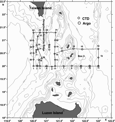
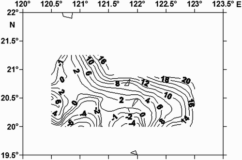
Figure 1 shows the bottom topography and locations of the hydrographic stations (◊) and Argo floats (○) in the computational region. In Fig. 1 Luzon Strait is located between Taiwan Island and Luzon Island, and numbers 15, 16, 17, 29, 30 and 32 identify the locations of the Argo floats. The other numbers identify the locations of the CTD sensors. The five Argo floats 2901169, 290170, 2901171, 2901172 and 2901167 (identified by a triangle in a circle) were deployed at locations 2, 4, 9, 10 and 11, respectively, during the October 2008 cruise.

Fig. 1 Bottom topography and locations of hydrographic stations (◊) and Argo floats (○), constructed in October 2008. The three boxes used for inverse analysis are also indicated.

2 Description of the diagnostic model

Assuming that the density field ρ is given, and the ß -effect is considered, as already discussed in Yuan and Su (1988), both the non-linear and lateral friction terms in the momentum equation are negligible. For circulation in the computational region (see Fig. 1), the dimensionless momentum equation in the x direction (e.g., Yuan et al., 2009) can be expressed by

where u, v and w are the velocity components along the x, y and z axes; the x axis points eastward; the y axis points northward; the z axis is directed vertically upward; t is time; p is pressure; and ρ ₀ is a constant density. The overbar over the variables denotes the dimensionless variables as follows:

The Rossby number R₀ and horizontal viscosity Ekman number E_m can be estimated as follows:

and

Here, the characteristic values of velocity U and the characteristic horizontal length L are set to 100 cm s⁻¹ and 3.5 × 10⁷ cm, respectively. The latter is approximately the width of Luzon Strait, f and f ₀ are both Coriolis parameters, f ₀ = 5.0 × 10⁻⁵ s⁻¹ (θ = 20.0°), A_z is the vertical kinematic eddy coefficient, and the horizontal viscosity coefficient is chosen as A_l  = 1 × 10⁸ cm² s⁻¹. Therefore, the time dependence of velocity, as well as the non-linear and horizontal viscosity friction terms in Eq. (1) are negligible.

Assuming a constant vertical eddy coefficient, A_z , and using a right-hand Cartesian coordinate system with the z-axis pointing upward, steady-state momentum and continuity equations can be derived (see Yuan et al., 1986, 2007 for more details), in which the Boussinesq approximation has been used. For boundary conditions at both the surface and the bottom, readers are referred to Yuan et al. (2007, 2008, 2009).

The governing equation for the streamfunction, ψ, can be further deduced by vertically integrating the momentum equation as follows (see Yuan et al., 2007, 2008):

In which

and

where ρ ₀ is a constant density, ρ and p are density and pressure anomalies, H is the sea depth, g is acceleration due to gravity; k is the unit vector along the axis z; is the gradient operator; , called the β-effect; u and v are the eastward and northward velocity components, respectively; and v (u, v) is the horizontal velocity vector. The wind stress vector is , and is the bottom friction stress vector. The vertically averaged horizontal velocity vector is V, B is the bottom friction coefficient, J is the Jacobian operator.

On the right-hand side of Eq. (2), the first term represents the joint effect of baroclinity and bottom topography (JEBAT), the second term represents the effect of wind stress rotation (WSR) and the third term represents the interaction between wind stress and bottom topography (IBWST). Mertz and Wright (1992) discussed in detail the physical interpretation of the JEBAT term, emphasizing that JEBAT might be regarded as a real forcing when the density field is specified, as is the case in the diagnostic model used for the present study. We rewrite Eq. (2) in the following form:

which can also be expressed as

where

and V ⁽ⁿ⁾ = V · n, where n is the unit vector normal to the contours of fH ⁻¹. As Mertz and Wright (1992) pointed out, when the density field is specified Eqs (5) and (6) emphasize the JEBAT term as a transport-generating term in that it enters Eq. (6) as a result of the depth-averaged flow across contours of fH ⁻¹, likewise for the IBWST term. The second term on the right-hand side of Eqs (5) and (6) is a resistance forcing of the flow across the contours of fH ⁻¹ as a result of the bottom friction. It can be seen from the estimation of orders of magnitudes that the first term on the right-hand side of Eq. (6) is dominant, while the second-order derivative terms are relatively small. Note that all the boundary conditions for the streamfunction ψ are open. In Eq. (2), all values at the open boundaries, including both barotropic and baroclinic transports, are given by the results from a modified inverse method (see Section 4a).

If ψ is known, with a constant vertical kinematic eddy viscosity coefficient A_z , the components of the horizontal velocity v(u,v) can be obtained from an analytical expression using the streamfunction (see Yuan et al., 2007, 2008). The horizontal velocity components can be divided into four parts:

where (u_τ ,v_τ ) are the surface Ekman velocity components subject to the wind stress τ , (u_G ,v_G ) are the geostrophic velocity components, (u_B ,v_B ) are the bottom Ekman velocity components, which are almost zero outside the bottom Ekman layer, and (u_I ,v_I ) are the velocity components resulting from baroclinic viscous effects. By definition, (u_I ,v_I ) are generally small, and they approach zero at the sea floor, as can be seen by comparing their magnitudes with the geostrophic velocity components (u_G ,v_G ). The explicit forms in Eqs (8a) and (8b) were discussed by Yuan et al. (2007, 2008).

3 Results from observations

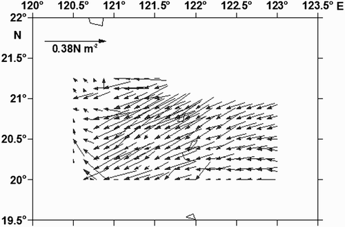
a Wind

The wind data used for this study were obtained from 5 to 20 October 2008 from the R/V Dong Fang Hong-2. The wind stress vector is computed from the wind velocity vector (u_s ,v_s ) using the formula:

where ρ_a  = 1.223 kg m⁻³ is the density of air at the surface, and C_d is the drag coefficient, equal to 1.3 × 10⁻³. Figure 2 shows the distribution of wind stress over the region studied. In Fig. 2 the wind data are interpolated to a regular grid. From this figure, one can see that the region is dominated by northeasterly winds except for a small region in the southeastern corner, where easterly winds prevail. The magnitude of the northeasterly wind stress can reach approximately 0.38 N m⁻², significantly larger than that of the easterly wind stress in the region.

Fig. 2 Wind stress (N m⁻²) distribution over the region studied during October 2008.

b Water Property Distribution

Because of space limitation, only the horizontal distributions of water temperature, salinity and density at 200, 400 and 600 m depths are presented here (see Figs 3, 4 and 5). In Figs 3, 4 and 5 the dots indicate where observations were made. In Fig. 5 the shaded area is where the water depth is less than 600 m.

Fig. 3 (a) Horizontal distribution of the water temperature (°C); (b) salinity (practical salinity scale used); and (c) density (σ_t ) at 200 m depth in the region studied during October 2008.

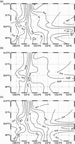
Fig. 4 As in Fig. 3 except at 400 m depth.

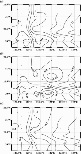
Fig. 5 As in Fig. 3 except at 600 m depth (grey denotes the sea bottom).

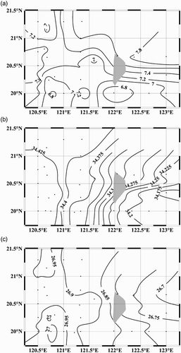
At 200 m depth (Fig. 3), one can see relatively high temperatures and salinity but low density in the area east of 122°00′E and in the northern part of the central area, representing the intrusion of Kuroshio water. In the southern and northern parts of the western area, water temperature and salinity are lower, and the density is higher, indicative of an origin in the SCS. At 400 m depth (Fig. 4), water temperature and salinity are higher, but density is lower in the eastern area, suggesting the presence of Kuroshio water. In the northern part of the middle area, temperature and salinity are slightly lower, but their lowest values are seen in the southern and northern parts of the western area, reflecting the strong influence of water originating in the SCS. The contrast in density is the opposite. The property distribution at 600 m (Fig. 5) shows higher temperature in the northeastern area and lower temperature and higher density near 122°00′E on the southern boundary. In the southern and northern parts of the western area, the temperature is lower, but salinity is higher, resulting in a relatively high density. Salinity is highest in the western area and lowest in the eastern area, consistent with the contrast in properties in intermediate water between the Pacific and the SCS (e.g., Chen & Wang, 1998; Qu, 2002).

Figures 6a and 6b show the temperature-salinity (T-S) diagram for the stations at the southern and northern boundaries of the region. For comparison, the mean T-S diagrams for areas marked in yellow and red are also included, representing the typical characteristics of the SCS (dashed yellow line) and upstream Kuroshio (dashed red line) water, respectively; data are from the World Ocean Atlas (WOA) climatology. These two curves intersect near σ _t ≈ 25.75 kg m⁻³, lying approximately at 300 m depth. From Fig. 6a one can see that water at the three stations west of 121°00′E near the southern boundary (approximately 20°00′N) has about the same characteristics as the SCS water, while water at stations east of 121°00′E is dominated by Kuroshio water. Similarly, Fig. 6b shows that water at the two stations west of 120°45′E near the northern boundary is mostly SCS water, while the influence of Korushio water becomes increasingly important as we progress to stations east of 120°45′E. This result implies that Kuroshio water is confined primarily to the east of 121°00′E near the southern boundary. From there, it flows northwestward through the stations east of 120°45′E near the northwestern boundary, in good agreement with the results of the diagnostic model discussed below.

Fig. 6 T-S diagram for the hydrographic stations at (a) the southern and (b) the northern boundary of the region. Mean T-S diagrams in the yellow and red areas are also included to represent the SCS (yellow dashed) and upstream Kuroshio (red dashed) water. Different colours and shapes are used to identify hydrographic stations and corresponding T-S profiles for (a) the southern boundary and (b) the northern boundary of the region. Contour lines indicate potential density (kg m⁻³). The practical salinity scale is used.

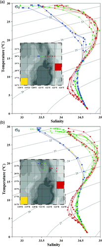
The hydrographic features discussed above have many similarities to those reported by Liang et al. (2008) at their stations L1 (20°47.7′N, 120°56.4′E), L2 (20°20.5′N, 120°54.3′E) and L3 (19°48.7′N, 120°56.4′E). The T-S curve was close to that of SCS water at L3 but gradually approached that of Kuroshio water as it moved north, implying that L3 may have been in proximity to the southern boundary of the Kuroshio intrusion (see Liang et al., 2008).

c Geostrophic Currents

In this section, we discuss the geostrophic currents of the region studied using sea level data (Fig. 7). The sea level anomalies and geostrophic currents were produced in France by the Archiving, Validation, and Interpolation of Satellite Oceanographic data (Aviso) project using the mapping method of Ducet et al. (2000). The data were archived in weekly (seven days) averaged frames (Ducet et al., 2000). The geostrophic currents were calculated from the absolute dynamic topography, which consists of a mean dynamic topography and the altimetric sea level anomalies (see Rio & Hernandez, 2004). The method of estimating a mean dynamic topography was explained in detail by Rio and Hernandez (2004).

Fig. 7 Geostrophic currents (cm s⁻¹) calculated from the merged absolute dynamic topography on (a) 15 October and (b) 17 December 2008. Data over the shelf shallower than 500 m have been masked.

Geostrophic currents calculated from the merged absolute dynamic topography (MADT) for the period 5–20 October 2008, are presented in Fig. 7a. In Fig. 7 M2 indicates the location of the mooring station, which is located at 20°59.961′N, 120°30.332′E during the days of observation from 25 April to 26 September 2008 (see Liao et al., 2010). From this figure, we can see that the intrusion of the Kuroshio current makes an anticyclonic meander through mooring station M2 (20°59.961′N, 120°30.332′E) in Luzon Strait, and from there most of the water turns northeastward into the region east of Taiwan. An anticyclonic eddy exists in the region west of 119°00′E and south of 22°00′N but does not seem to have any connection to the intrusion of the Kuroshio. Part of the Kuroshio water intrudes northwestward through section 120°00′E. Then, meanders cyclonically and continues to flow westward into the interior SCS, consistent with earlier studies (e.g., Centurioni et al., 2004; Yuan et al., 2008; Liang et al., 2008). The current on 17 December 2008 (Fig. 7b) shows essentially the same pattern. Both patterns are forced by the northeasterly wind.

4 Results from a diagnostic model

a Velocity Distribution Determined by MIM

In order to solve Eq. (2) for the streamfunction ψ, we need to know its open boundary conditions. As mentioned above, values at the open boundaries are determined by a modified inverse method (MIM). The modified inverse method described in Yuan et al. (1992) is used to compute the sectional distributions of velocity and volume transport in the computational region (Fig. 1). In this method, the following three assumptions are made:

1.	The vertical friction term in the momentum equation is retained.
2.	All convection terms and the vertical diffusion term in the density and salinty (temperature) equations are retained, but the horizontal diffusion terms are negligible.
3.	The ß-effect is considered.

In this computation, the wind speed data must be given. Three boxes are chosen to perform the MIM (Fig. 1). Each box is divided vertically into five layers with isopycnal surfaces, σ _t,s,p, at 25.0, 27.0, 30.0 and 35.0 kg m⁻³ as the four inter-surfaces. Yuan et al. (1986, 1992) conducted a set of numerical experiments using values of 10, 50 and 100 cm² s⁻¹ for the vertical kinematic eddy coefficient, A_z . Their results indicated that A_z  = 100 cm² s⁻¹ is the best choice for the region studied. They also found that the horizontal velocity components, u and v, are not sensitive to A_z . Thus, the vertical kinematic eddy coefficient A_z is simply set to 100 cm² s⁻¹. In the density and salinity (temperature) equations the vertical diffusivity eddy coefficient K_v is set to 10 cm² s⁻¹ (e.g., Yuan et al., 1992; Liu et al., 2000). For the choice of an optimum reference level, we used the method of Fiadeiro and Veronis (1982); the velocity at the optimum reference level is unknown and can be obtained from the solution of the MIM equation.

In the following we discuss the sectional velocity distributions at sections 1–11, 14–18 and 21–24 (Fig. 1). It is worth noting that (1) the perpendicular component of the horizontal velocity to each section can only be obtained from the MIM; and (2) the perpendicular component of horizontal velocity obtained from the MIM includes the geostrophic and non-geostrophic components, in which the values of the geostrophic component are generally much greater than those for the non-geostrophic component (such as the surface Ekman velocity component subject to the wind stress τ) except for the bottom Ekman layer.

1 Section 1–11

Section 1–11 is a latitudinal section at about 20.0°N, the southern boundary of the region studied (Fig. 1). Two velocity cores representing the Kuroshio current are visible across this section (Fig. 8a). The western core is located between 121°08′ and 121°35′E, consistent with the T-S diagram shown in Fig. 6. This core extends to about 400 m, with its maximum velocity exceeding 120 cm s⁻¹ at the surface. The eastern core is located between 122°00′ and 122°25′E, with its maximum velocity exceeding 60 cm s⁻¹ at the surface.

Fig. 8 Sectional distributions of velocity (cm s⁻¹) at latitudinal (a) section 1–11, (b) section 14–18, and (c) section 21–24 determined by the modified inverse method in October 2008. Positive values indicate northward flow.

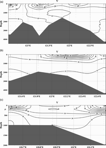
2 Section 14–18

Section 14–18 is an approximately latitudinal section extending from 20.30° to 20.38°N near the northeastern boundary of the region studied (Fig. 1). Across this section one can see a velocity core of the Kuroshio current lying at 122°06′ to 122°20′E. Its maximum velocity exceeds 90 cm s⁻¹ at the surface. After an eastern branch of the Kuroshio current crosses section 1–11 (Fig. 8a), it continues to flow northwestward, with its core at about 122°12′E through section 14–18.

3 Section 21–24

Section 21–24 is a latitudinal section at about 21.20°N, near the northwestern boundary of the region studied (Fig. 1). Two velocity cores of the Kuroshio current are seen in this section. The western core is located west of 120°45′E, with its maximum velocity exceeding 90 cm s⁻¹ at the surface. In the vertical, this velocity core extends to about 400 m. The eastern core is located east of 121°05′E, with its maximum velocity exceeding 100 cm s⁻¹ at the surface. Apparently, the eastern core of the Kuroshio current is somewhat stronger than the western core. After crossing section 1–11 (Fig. 8a), both cores flow northwestward at sections 14–18 and 21–24 (Figs 8b and 8c).

b Streamfunction and Volume Transports

The diagnostic model domain is shown in Fig. 1. The horizontal grid sizes are Δy = 28.03 km, Δx = Δy cos θ = 28.03 cos θ km, where θ is the latitude. At θ = 20.5°, f = 5.107 × 10⁻⁵ s⁻¹ and β = 2.133 × 10⁻¹¹ s⁻¹ m⁻¹. Based on the results of Yuan et al. (2007, 2008, 2009), the vertical kinematic eddy coefficient A_z is chosen to be 100 cm² s⁻¹. Different values of the bottom friction coefficient, B, between 1 × 10⁻² and 5 × 10⁻² m s⁻¹ are used. In the following, only results with B = 1 × 10⁻² m s⁻¹ are discussed (Yuan et al., 2007, 2009). All values at the open boundaries of Eq. (2) were provided by the results from a MIM in Section 4a and the streamfunction distribution ψ can be solved numerically.

Figure 9 shows the distribution of the streamfunction and volume transport in October 2008. The main stream of the Kuroshio current is seen at 122°10′ to 122°40′E near the southern boundary. It flows northwestward through section 21–24 (the northwestern boundary), in good agreement with the results from the MIM. There is a cyclonic eddy west of the main stream of the Kuroshio near the southern boundary, consistent with the horizontal distribution of water temperature and density at 400 and 600 m depths. There is also a cyclonic eddy at 121°00′E near the southern boundary. The western branch of the Kuroshio discussed above (Fig. 8) is not visible in Fig. 9 because it extends to only about 400 m.

Fig. 9 Distribution of streamfunction and volume transport (Sv) in the study region in October 2008.

If the horizontal velocity vector v(u,v) is known, the volume transports Q(φ) across the longitudinal section φ = 120°45′E south of Taiwan satisfies the following formula,

where y ₁ (θ ₁) and y ₂ (θ ₂) are the intersections between the longitudinal section 120°45′E and section 1–6 and section 21–24, respectively, of the study region (see Fig. 1), and z ₁ and z ₂ are the ocean's surface and bottom, respectively. The volume transport, Q, across the above longitudinal section south of Taiwan is about 4 Sv.

c Circulation System in the Upper 400 m

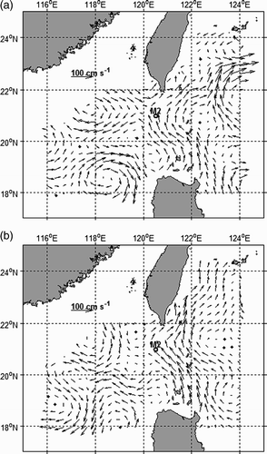
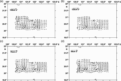
Figures 10a and 10b show the surface currents from the ADCP measurements and the diagnostic model, respectively. Qualitatively, the two patterns agree well. Figures 11a to 11d show the subsurface currents from the diagnostic model at 100, 200, 300 and 400 m depths. The intrusion of the Kuroshio is obvious, with a maximum velocity of 175 cm s⁻¹ near the surface. The main stream of the Kuroshio is located at 122°10′E to 122°40′E and flows northwestward near the southern boundary. Its western branch is seen at 121°00′E to 121°35′E but is primarily confined to the upper 400 m (Figs 10b and 11a to 11d). From there, it crosses the northern boundary east of 120°45′E and intrudes northwestward into the interior of the SCS, consistent with the T-S diagrams discussed in Section 3 (Fig. 6) as well as the geostrophic currents shown above (Fig. 7). Two cyclonic eddies are seen near the southern boundary (Figs 11c and 11d).

Fig. 10 (a) Currents determined from ADCP measurements in the surface layer (8–24.7 m) and (b) velocity vectors (cm s⁻¹) at 10 m determined by the diagnostic model of the study region during October 2008.

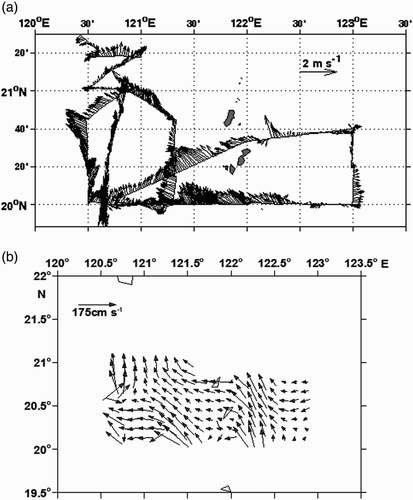
Fig. 11 As in Fig. 10b except at (a) 100 m, (b) 200 m, (c) 300 m and (d) 400 m depths.

The implication of these results is that the geostrophic velocity components are the dominant terms except for the bottom Ekman layer, and their magnitudes are much greater than those of the surface Ekman velocity components, as already pointed out by Yuan et al. (2007, 2008).

d Circulation System Below 400 m

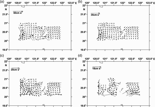
Figures 12a to 12d show the circulation from the diagnostic model at the 500, 700, 1000 and 1500 m levels in the study region. The main stream of the Kuroshio is confined to the upper 700 m. At depths between 700 and 1500 m (say 1000 m), the flow is predominantly southwestward or westward in the area north of 20°30′N, while southeastward flow dominates in the area south of 20°30′N. A cyclonic eddy is evident in the area east of Luzon Strait. Cyclonic eddies are seen on both sides of Luzon Strait at depths around 1500 m.

Fig. 12 As in Fig. 11 except at (a) 500 m, (b) 700 m, (c) 1000 m and (d) 1500 m depths.

e Comparison with the Trajectories of Argo Floats

Five Argo floats, 2901169, 290170, 2901172, 2901171 and 2901167, were deployed at 20°N, 120°45′E; 20°N, 121°13′E; 20°N, 122°20′E; 20°N, 122°40′E and 20°N, 123°0′E, respectively, during the October 2008 cruise. Float 2901169 first moved northwestward or northward from 7 October to 18 December 2008 (Fig. 13a) and then northeastward into the area southwest of Taiwan. Of the five Argo floats deployed, Argo float 2901172 was the only one that flowed westward across Luzon Strait into the SCS, thus, particular attention is paid to the trajectories of Argo float 2901172 in the following.

Fig. 13 (a) Trajectories of Argo floats 2901169, 290170, 2901171, 2901172 and 2901167 for the period 7 October to 18 December 2008 (▴: 7 October 2008; ⋆: 18 December 2008); (b) trajectory of Argo float 2901172 for the period 9 October 2008 to 7 January 2009 (green lines with solid dots: at the surface; red lines: at 1000 m; ▴: 9 October 2008; ⋆: 7 January 2009); (c) trajectory of the five Argo floats for the period 7 October 2008 to 5 January 2009 (▴: 7 October 2008; ⋆: 5 January 2009); and (d) trajectory of Argo float 2901172 for the period 9 October 2008 to 2 January 2010 (green lines with solid dots: at the surface; red lines: at 1000 m; ▴: 9 October 2008; ⋆: 2 January 2010).

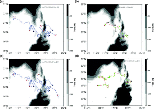
As float 2901172 approached 20°30′N to 21°00′N, 120°30′E to 121°15′E, it surfaced near 20°35′N, 121°10′E, and then flowed west-northwestward with the Kuroshio through Luzon Strait. This float then descended to a depth of about 1000 m and continued northwestward to 120°50′E, 20°40′N and finally entered the SCS. These trajectories resemble the results from the diagnostic model discussed above.

We further investigated the flow of Argo float 2901172 during two periods, one when the float drifted at the surface (period 1) and the other when the float drifted at 1000 m depth (period 2).

Figure 13b shows the trajectory of Argo float 2901172 during period 1, from 9 October to 28 December 2008. From October to December, northeasterly winds prevailed, which provided favourable conditions for float 2901172 to move westward across Luzon Strait at the surface. Results from the diagnostic model confirmed that the flow in the area (20°20′ to 21°00′N, 120°45′ to 121°50′E) was dominated by a west-northwestward flow at the surface (Figs 7a and 7b, Fig. 10 and Fig. 11). On 18 December 2008, float 2901172 was seen at O1 (20°25′N, 121°00′E) (Fig. 13b). The northwestward flow at the surface forced it to move northwestward toward Luzon Strait, from position O1 (20°25′N, 121°00′E) to position O2 (20°45′N, 120°50′E) (Fig. 13b). Then, the float descended to a depth of about 1000 m and entered period 2. As results from the diagnostic model have indicated, the flow at 1000 m was dominated by a west-southwestward flow in the area north of 20°30′N. This flow forced float 2901172 to move across Luzon Strait from position O2 (20°45′N, 120°50′E) to position O3 (21°00′N, 120°06′E) from 19 December to 28 December 2008 (Fig. 13b). The trajectories of floats 2901167, 2901169, 2901170, 2901171 and 2901172 from 7 October 2008 to 5 January 2009, and float 2901172 from 9 October 2008 to 6 January 2010, are also included (Figs 13c and 13d), showing a consistent flow pattern as discussed above.

5 Conclusions

On the basis of ADCP current measurements and hydrographic data, a diagnostic model with a modified inverse method has revealed some new features of the circulation in Luzon Strait in October 2008. A summary of the results follows.

1.	The main stream of the Kuroshio current is located at 122°10′E to 122°40′E and flows northwestward near the southern boundary, confined to the upper 700 m. Its western branch is seen at 121°00′E to 121°35′E and is primarily confined to the upper 400 m. From there, it crosses the northern boundary east of 120°45′E and intrudes northwestward into the interior SCS, consistent with the T-S diagrams as well as the geostrophic currents calculated from the MADT. Two cyclonic eddies are seen near the southern boundary.
2.	At depths between 700 and 1500 m (say 1000 m), the flow is predominantly southwestward or westward in the area north of 20°30′N, while southeastward flow dominates in the area south of 20°30′N. A cyclonic eddy is evident in the area east of Luzon Strait. Cyclonic eddies are seen on both sides of Luzon Strait at depths around 1500 m.
3.	The volume transport across longitudinal section 120°45′E between about 20.00°N and 21.20°N south of Taiwan during the period of observation was about 4 Sv.
4.	From October to December, northeasterly winds prevailed, and this provided favourable conditions for float 2901172 to move westward across Luzon Strait at the surface. Both the flow at the surface in the area (20°20′ to 21°00′N, 120°45′ to 121°50′E) and the flows at the 1000 m level in the area north of 20°30′N, forced float 2901172 to move across Luzon Strait into the SCS during October to December 2008.

Acknowledgements

This work was supported by the National Basic Research Program of China (No. 2007 CB816003), the International Cooperative Project of the Ministry of Science and Technology of China (No. 2006DFB21630), the key project of the National Natural Science Foundation of China (No. 40520140073 and No. 41176020) and the National Basic Research Program of China (No. 2011CB403503). We wish to thank the crew and participants of the R/V Dong Fang Hong-2 for their support and cooperation. Two anonymous reviewers made very valuable comments and suggestions, which were extremely helpful in the revision of our manuscript. The authors are greatly indebted to them for their detailed and careful comments and help.

References

- Cai , S. Q. , Liu , H. L. , Li , W. and Long , X. M. 2005 . Application of LICOM to the numerical study of the water exchange between the South China Sea and its adjacent oceans . Acta Oceanologica Sinica , 24 ( 4 ) : 10 – 19 .
- Centurioni , L. R. , Niiler , P. P. and Lee , D. K. 2004 . Observation of inflow of Philippine Sea surface water into the South China Sea through the Luzon Strait . Journal of Physical Oceanography , 34 : 113 – 121 . (doi:10.1175/1520-0485(2004)034<0113:OOIOPS>2.0.CO;2)
- Chen , C. T. and Wang , S. L. 1998 . Influence of the intermediate water in the western Okinawa Trough by the outflow from the South China Sea . Journal of Geophysical Research , 103 : 12683 – 12688 . (doi:10.1029/98JC00366)
- Chu , P. and Li , R. 2000 . South China Sea isopycnal-surface circulation . Journal of Physical Oceanography , 30 : 2419 – 1438 . (doi:10.1175/1520-0485(2000)030<2419:SCSISC>2.0.CO;2)
- Ducet , N. , Le Traon , P.-Y. and Reverdin , G. 2000 . Global high resolution mapping of ocean circulation from TOPEX/Poseidon and ERS-1/2 . Journal of Geophysical Research , 105 : 19477 – 19498 . (doi:10.1029/2000JC900063)
- Fang , G. H. , Wei , Z. X. , Choi , B. H. , Wang , K. , Fang , Y. and Li , W. 2003 . Interbasin freshwater, heat and salt transport through the boundaries of the East and South China Seas from a variable-grid global ocean circulation model . Science in China, Series D: Earth Sciences , 46 ( 2 ) : 149 – 161 . (doi:10.1360/03yd9014)
- Fiadeiro , M. E. and Veronis , G. 1982 . On the determination of absolute velocities in the ocean . Journal of Marine Research , 40 ( Suppl ) : 159 – 182 .
- Liang Wen-Der , Y. J. , Yang , T. Y. , Tang , W. S. and Chuang . 2008 . Kuroshio in the Luzon Strait . Journal of Geophysical Research , 113 : 1–19, C08048 doi:10.1029/2007JC004609
- Liao , G. H. , Yuan , Y. C. and Xu , X. H. 2007 . Diagnostic calculation of the circulation in the South China Sea during summer 1998 . Journal of Oceanography , 63 ( 2 ) : 161 – 178 . (doi:10.1007/s10872-007-0019-4)
- Liao , G. H. , Yuan , Y. C. and Xu , X. H. 2008 . Three dimensional diagnostic study of the circulation in the South China Sea during winter 1998 . Journal of Oceanography , 64 ( 5 ) : 803 – 814 . (doi:10.1007/s10872-008-0067-4)
- Liao , G. H. , Yuan , Y. C. , Kaneko , A. , Yang , C. H. , Chen , H. , Taniguchi , N. , Gohda , N. and Minamidate , M. 2010 . Analysis on internal tidal characteristics in the layer above 450 m from ADCP observation in the Luzon Strait . Science China (Series D) , doi: 10.1007/s11430-010-4102-0
- Liu , Y. G. , Yuan , Y. C. , Su , J. L. and Jiang , J. Z. 2000 . Circulation in the South China Sea in summer 1998 . Chinese Science Bulletin , 45 ( 18 ) : 1648 – 1655 . (doi:10.1007/BF02898979)
- Mertz , G. and Wright , D. G. 1992 . Interpretations of the JEBAR term . Journal of Physical Oceanography , 22 : 301 – 305 . (doi:10.1175/1520-0485(1992)022<0301:IOTJT>2.0.CO;2)
- Qu , T. 2000 . Upper layer circulation in the South China Sea . Journal of Physical Oceanography , 30 : 1450 – 1460 . (doi:10.1175/1520-0485(2000)030<1450:ULCITS>2.0.CO;2)
- Qu , T. D. 2002 . Evidence for water exchange between the South China Sea and the Pacific Ocean through the Luzon Strait . Acta Oceanologica Sinica , 21 ( 2 ) : 175 – 185 .
- Qu , T. , Kim , Y. Y. , Yaremchuk , M. , Tozuka , T. , Ishida , A. and Yamagata , T. 2004 . Can Luzon Strait transport play a role in conveying the impact of ENSO to the South China Sea? . Journal of Climate , 17 : 3644 – 3657 . (doi:10.1175/1520-0442(2004)017<3644:CLSTPA>2.0.CO;2)
- Qu , T. , Song , Y. T. and Yamagata , T. 2009 . An introduction to the South China Sea throughflow: Its dynamics, variability, and application for climate . Dynamics of Atmospheres and Oceans , 47 : 3 – 14 . (doi:10.1016/j.dynatmoce.2008.05.001)
- Rio , M. H. and Hernandez , F. 2004 . A mean dynamic topography computed over the world ocean from altimetry, in situ measurements, and a geoid model . Journal of Geophysical Research , 109 : C12032 doi:10.1029/2003JC002226
- Yaremchuk , M. and Qu , T. 2004 . Seasonal variability of the circulation near the Philippine coast . Journal of Physical Oceanography , 34 : 844 – 855 . (doi:10.1175/1520-0485(2004)034<0844:SVOTLC>2.0.CO;2)
- Yuan , Y. C. and Su , J. 1988 . The calculation of Kuroshio Current structure in the East China Sea—early Summer 1986 . Progress in Oceanography , 21 : 343 – 361 . (doi:10.1016/0079-6611(88)90013-4)
- Yuan , Y. C. , Su , J. L. and Xia , S. Y. 1986 . A diagnostic model of summer on the northwest of the East China Sea . Progress in Oceanography , 17 : 163 – 176 . (doi:10.1016/0079-6611(86)90042-X)
- Yuan , Y. C. , Su , J. L. and Pan , Z. Q. 1992 . Volume and heat transports of the Kuroshio in the East China Sea in 1989 . La mer , 30 : 251 – 262 .
- Yuan , Y. C. , Liao , G. H. and Xu , X. H. 2007 . Three dimensional diagnostic modeling study of the South China Sea circulation before onset of summer monsoon in 1998 . Journal of Oceanography , 63 ( 1 ) : 77 – 100 . (doi:10.1007/s10872-007-0007-8)
- Yuan , Y. C. , Liao , G. H. , Guan , W. B. , Wang , H. Q. , Lou , R. Y. and Chen , H. 2008 . The circulation in the upper and middle layers of the Luzon Strait during spring 2002 . Journal of Geophysical Research , 113 : 1–18, C06004 doi:10.1029/2007JC004546
- Yuan , Y. C. , Liao , G. H. and Yang , C. H. 2009 . A diagnostic calculation of the circulation in the upper and middle layers of the Luzon Strait and the northern South China Sea during March 1992 . Dynamics of Atmospheres and Oceans , 47 : 86 – 113 . (doi:10.1016/j.dynatmoce.2008.10.005)